A Criterion for Rating the Usability and Accuracy of the One-Diode Models for Photovoltaic Modules

Abstract

In selecting a mathematical model for simulating physical behaviours, it is important to reach an acceptable compromise between analytical complexity and achievable precision. With the aim of helping researchers and designers working in the area of photovoltaic systems to make a choice among the numerous diode-based models, a criterion for rating both the usability and accuracy of one-diode models is proposed in this paper. A three-level rating scale, which considers the ease of finding the data used by the analytical procedure, the simplicity of the mathematical tools needed to perform calculations and the accuracy achieved in calculating the current and power, is used. The proposed criterion is tested on some one-diode equivalent circuits whose analytical procedures, hypotheses and equations are minutely reviewed along with the operative steps to calculate the model parameters. To assess the achievable accuracy, the current-voltage (I-V) curves at constant solar irradiance and/or cell temperature obtained from the analysed models are compared to the characteristics issued by photovoltaic (PV) panel manufacturers and the differences of current and power are calculated. The results of the study highlight that, even if the five parameter equivalent circuits are suitable tools, different usability ratings and accuracies can be observed.

1. Introduction

In the field of photovoltaics, the diode-based equivalent circuits of photovoltaic (PV) cells and modules have been widely used because they allow the designer to optimize the system performance and maximize the effectiveness of the economic investment. The use of accurate models of the electrical behaviour of PV modules, which is obviously important to implement simulation tools, is also required to test the dynamic performances of the inverters equipped with the maximum power point tracker (MPPT). In order to get results, which would be confirmed by experimental measurements, the practical effectiveness of MPPT control algorithms was analysed using different diode-based equivalent circuits [1,2,3]. It was observed that the study of the transient conditions, which are quite common for an MPPT, requires very reliable equations describing the behaviour of the PV array working far from the standard rating conditions [4].

Usability and accuracy, which have been already addressed by other authors [5], are important features that have to be carefully considered before deciding the mathematical model to be adopted to simulate the electrical behaviour of PV devices. The usability is mainly affected by the mathematical difficulties, which may be encountered in performing calculations, and the unavailability of the performance data used to evaluate the model parameters. Before starting working, it would be preferable to have a clear idea about the need of specific performance data, which may be not available or difficult to extract from the issued datasheets, and the computation difficulties, which may require the use of mathematical tools ranging from simple algorithms to complex methods implemented in dedicated computational software. Also the accuracy is a relevant parameter, even though its achievable level may significantly depend on the physical characteristics of the modelled PV devices.

To better understand the origin of the diode-based equivalent circuits used for modelling PV devices it is useful to remember that, like a semiconductor diode, a PV cell consists of two layers of semiconductor material, usually silicon, differently doped, that are electrically connected to two metallic electrodes deposited on their outer surfaces. To better understand the origin of the diode-based equivalent circuits used for modelling PV devices it is useful to remember that a PV cell is a diode made with two layers of semiconductor material, usually silicon, differently doped, that are electrically connected to two metallic electrodes deposited on their outer surfaces. It is well-known [2,6] that the absorption of light in semiconductors can, under certain conditions, create an electric current due to the capability of the absorbed photons of converting fixed electrons in freely moving conduction electrons.

A silicon PV cell shares with semiconductor electronic devices, such as diodes and transistors, the same processing and manufacturing techniques used to create p-n junctions. An ideal PV cell behaves like an illuminated semiconductor diode whose I-V characteristic was described by Shockley [7] with the following equation:

$$I=I_L-I_0\left(e^{\frac{qV}{\mathsf{\gamma }kT}}-1\right)$$

(1)

where I and V are the current and voltage, I_L is the photocurrent generated by illumination, I₀ is the reverse saturation current of the diode, q is the electron charge (1.602 × 10⁻¹⁹ C), k is the Boltzmann constant (1.381 × 10⁻²³ J/K), T is the junction temperature and diode ideality factor γ, in compliance with the traditional theory of semiconductors [8], is 1 for germanium and approximately 2 for silicon.

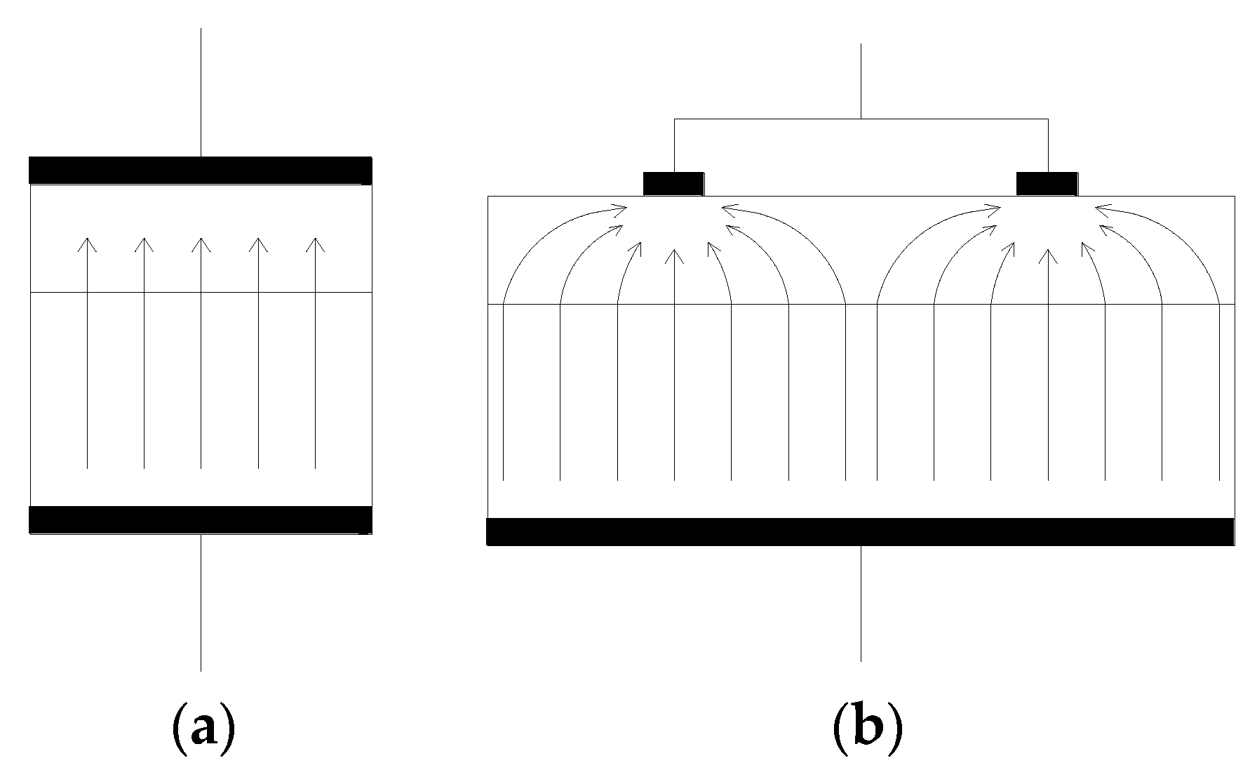
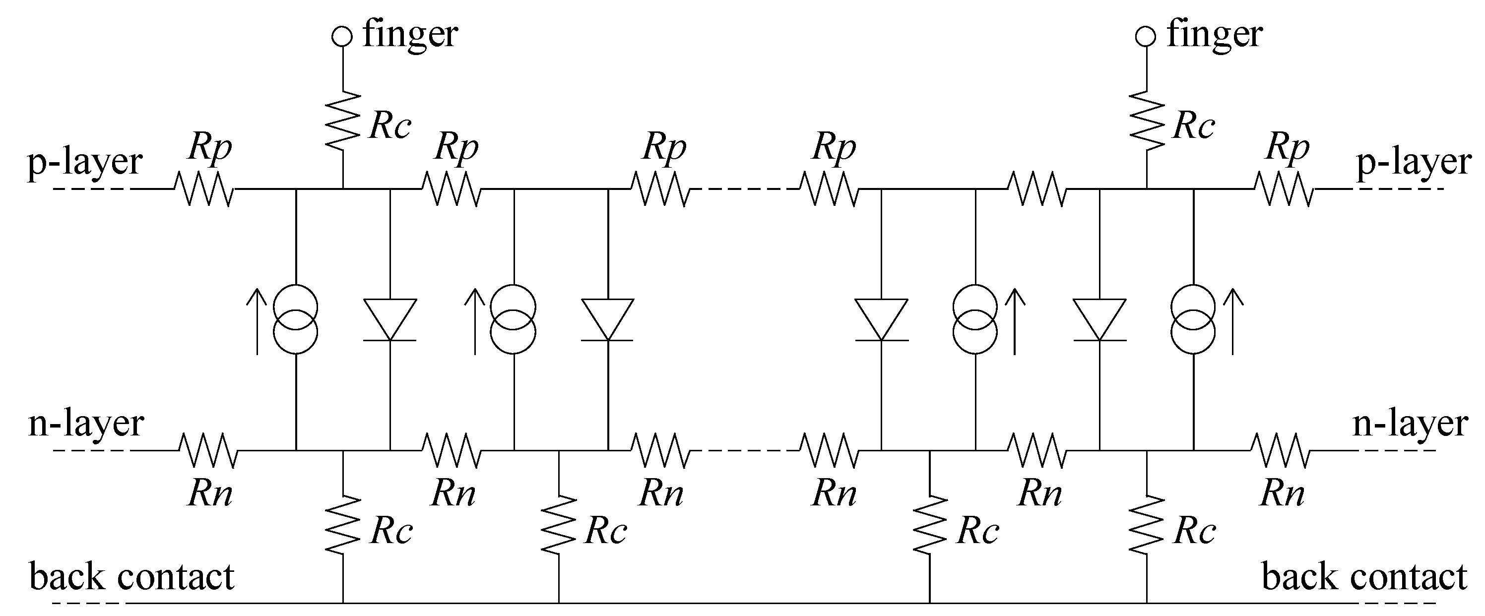
Wolf [9] observed that in a PV cell the photocurrent is not generated by only one diode but it is the global effect of the presence of a multitude of elementary flanked diodes that are uniformly distributed throughout the surface that separates the two semiconductor slabs of the p-n junction. The assertion of Wolf arises from a significant difference between diodes and PV cells: unlike semiconductor diodes, the upper electrode of a PV cell is deposited with a discontinuous structure that embeds several metal elements (fingers), whose shape and size are chosen with the aim of maximizing the absorbing surface and minimizing the contact resistance between fingers and silicon. In a real diode the electrodes face each other and the carriers of electricity flow through the silicon slabs following linear paths, which are perpendicular to the junction. In contrast, into a PV cell, because of the discrete shape of the upper electrode, the carriers of electricity follow curved paths toward the fingers that collect them (Figure 1).

As a result of the unequal length of the current paths, the carriers of electricity flow through different thicknesses of semiconductor and different electrical resistances are thus opposed. As consequence, each elementary portion of the p-n junction has a different electrical behaviour and, in turn, a different I-V characteristic. In order to get a realistic representation, a PV cell may be approximated with the distribute constants electric circuit of Figure 2, which contains a multitude of elementary lumped components composed of a current generator and a diode. Numerous electrical resistances take account of various dissipative effects. Major contributions to the internal series resistance come from the sheet resistance of the p-layer, the bulk resistance of the n-layer and the resistance between the semiconductor layers and the metallic contacts.

The elementary diodes are inter-connected by resistors R_p and R_n, which represent the transverse distributed resistances of p-layer and n-layer, respectively; resistors R_c are included to consider the contact resistance between the semiconductor and the fingers, or the back contact. Because such equivalent circuit would be too complex to be used, simplified equivalent circuits, which contain one or two diodes, a current generator and two resistors, were considered.

Many authors have proposed analytical procedures for determining the model parameters on the basis of the performance data usually provided by manufactures [10,11,12,13,14,15,16,17,18,19,20,21,22,23,24,25,26,27,28,29,30,31,32,33,34,35,36,37,38,39,40,41,42,43,44,45,46,47,48,49,50,51,52,53,54,55,56,57]. The identification of the parameters contained in the diode-based equivalent circuits has been also tackled exploring the possibility of using different procedures such as Lambert W-function, evolutionary algorithms, Padè approximants, genetic algorithms, cluster analysis, artificial neural networks, harmony search-based algorithms and small perturbations around the operating point [58,59,60,61,62,63,64,65,66,67,68,69]. One-diode and two-diode models have been also used to describe the electrical behaviour of PV modules built with different technologies, such as thin-film PV cells and panels [17,18,47,49,66,70,71,72,73,74,75,76,77,78,79,80,81,82].

Because of the amount of combinations that can be obtained by changing the used set of performance data, the adopted hypotheses and the analytical procedures for evaluating the model parameters, a great number of one-diode models have been reported in the scientific literature. The selection of the model fit for purpose may be a difficult task, which cannot disregard some important aspects, such as:

• the kind and availability of the performance data used by the model;
• the reliability of the hypotheses on which the model is based;
• the procedure followed to obtain the expressions used to calculate the model parameters;
• the mathematical methods, tools and/or computer routines required to solve the equation system;
• the robustness and stability of the mathematical approach;
• the achievable precision of the model.

The features mentioned above affect the model effectiveness and change its usability rating and accuracy level. The usability is a qualitative parameter, whereas the accuracy achievable by a model requires a quantitative assessment. An aware choice of the one-diode model, which should be the best compromise between analytical complexity and expected accuracy, would require the capability of performing the complex synthesis of both qualitative and quantitative features. In order to help researchers and designers, working in the area of photovoltaic systems, to select the model fit for purpose, the usability and accuracy of some of the most famous one-diode models are overviewed and rated in this study. The paper is organised as follows: Section 2 presents the five-parameter equivalent circuit. To assess the usability rating the analytical procedures of some one-diode models are synthetically reviewed in Section 3 along with the used performance data, the required mathematical tools and the operative steps to obtain the model parameters. In Section 4, the accuracy of the tested one-diode models is evaluated by calculating the I-V characteristics of some PV modules and comparing them with the performance curves issued by manufacturers. A criterion for rating the usability and accuracy of the analysed one-diode models is presented in Section 5. Moreover, the model, which represents the ideal compromise between the usability and accuracy is highlighted. The appendix lists the detailed descriptions of the procedures used by the ranked models and the explicit or implicit expressions necessary to evaluate the model parameters; such a review also contains the sequence of operative steps to easily calculate the model parameters.

2. The One-Diode Equivalent Circuit

The one-diode equivalent circuit depicted in Figure 3 is characterized by five parameters, which are photocurrent I_L, diode reverse saturation current I₀, series resistance R_s, shunt resistance R_sh, and diode quality factor n = aN_csk/q, in which a is the shape factor, N_cs is the number of cells of the panel that are connected in series, q is the electron charge (1.602 × 10⁻¹⁹ C) and k is the Boltzmann constant (1.381 × 10⁻²³ J/K).

The one-diode model is described by the well-known equation:

$$I=I_L-I_0\left(e^{\frac{V+I{R}_s}{nT}}-1\right)-\frac{V+I{R}_s}{R_{sh}}$$

(2)

where T is the cell temperature. Following the traditional theory, the photocurrent depends on the solar irradiance and the diode reverse saturation current is affected by the cell temperature. The values of R_s, R_sh, n and I₀ variously affect the I-V characteristic of the PV panel [83]. The series and shunt resistances take account of dissipative phenomena and parasitic currents within the PV panel.

At a constant value of the solar irradiance, the internal dissipation of energy is reduced if the series resistance is lowered and/or the shunt resistance is increased. As a consequence, the panel becomes more efficient because the maximum power point (MPP) slides towards right and the I-V curve becomes sharper. Thin-film PV cells and modules, which present significant values of R_s and R_sh due to the use of materials that are more energy dissipative than the mono or poly crystalline silicon, are usually characterized by smooth I-V curves.

The analytical procedures proposed to calculate the five-parameter model generally require the following data, some of them are provided by the manufacturer datasheets:

• open circuit voltage V_oc,ref and short circuit current I_sc,ref at the standard rating conditions (SRC): irradiance G_ref = 1000 W/m², cell temperature T_ref = 25 °C and average solar spectrum at AM 1.5;
• voltage V_mp,ref and current I_mp,ref in the MPP at the SRC;
• open circuit voltage temperature coefficient μ_V,oc and short circuit current temperature coefficient μ_I,sc;
• number N_cs of series connected PV cells;
• the derivative of the I-V curve calculated at the maximum power, short circuit and open circuit points.

Because of the presence of current I in both terms of transcendent Equation (2), the solution of the five-equation system, which is necessary to calculate the model parameters, cannot be faced by means of exact mathematical methods. For this reason, both numerical calculation techniques and approximate forms of the equations were adopted.

3. Usability of the One-Diode Models

The models proposed by Hadj Arab et al. [24], De Soto et al. [25], Sera et al. [26], Villalva et al. [27], Lo Brano et al. [29], Seddaoui et al. [35], Siddique et al. [49], Yetayew et al. [52] and Orioli et al. [44] were selected in order to assess the effectiveness of the proposed criterion. The models are based on some fundamental equations that, for the first time, Kennerud [84], Phang et al. [85] and de Blas et al. [23] described even more than 30 years ago. Unfortunately, such early models were not conceived to allow a complete representation of the I-V characteristic for values of the solar irradiance and cell temperature different from the SRC.

To assess the usability rating of a procedure, which may be significantly lowered by the difficulties encountered in using it, it is necessary to explore the complete sequence of operative steps that permit to reach the wished results. Some of the analysed procedures evaluate the model parameters on the basis of similar information, but they adopt different simplifying hypotheses to solve the equations and/or do not use the same relations to describe the dependence on the cell temperature and/or the solar irradiance. A synthetic description of the used information, simplifying hypotheses and solving techniques is contained in the following paragraphs; the analytical procedures to calculate the model parameters are minutely described in the appendix.

3.1. Hadj Arab, Chenlo and Benghanem Model (Link 4)

The model Hadj Arab et al. [20] uses the following information:

• short circuit point [I = I_sc,ref; V = 0];
• open circuit point [I = 0; V = V_oc,ref];
• derivative of current at the short circuit point [∂I/∂V = −1/R_sho at I = I_sc,ref; V = 0];
• derivative of current at the open circuit point [∂I/∂V = −1/R_so at I = 0; V = V_oc,ref];
• MPP [I = I_mp,ref; V = V_mp,ref];

and assumes the following hypotheses:

$$\begin{array}{l}{e}^{\frac{V_{oc,ref}}{n{T}_{ref}}}>>e^{\frac{I_{sc,ref}{R}_s}{n{T}_{ref}}}\frac{I_{0,ref}}{n{T}_{ref}}{e}^{\frac{V_{oc,ref}}{n{T}_{ref}}}>>\frac{1}{R_{sh}}\\ R_s<<R_{sh}\frac{I_{0,ref}}{n{T}_{ref}}{e}^{\frac{I_{sc,ref}{R}_s}{n{T}_{ref}}}<<\frac{1}{R_{sh}}-\frac{1}{R_{sho}-R_s}\end{array}$$

(3)

The model parameters can be calculated using the explicit equations described in the appendix.

3.2. De Soto, Klein and Beckman Model (Link 5)

The model of De Soto et al. [25] is based on the following information:

(1)

short circuit point [I = I_sc,mrf; V = 0];

(2)

open circuit point [I = 0; V = V_oc,ref];

(3)

MPP [I = I_mp,ref; V = V_mp,ref];

(4)

derivative of power at the MPP [∂P/∂V = 0; V = V_mp,ref];

(5)

open circuit point with a cell temperature different from the SRC [I = 0; V = V_oc; G = G_ref; T ≠ T_ref].

No simplifying hypothesis is assumed. To simultaneously solve the system of five equations described in the appendix, De Soto et al. use a non-linear equation solver, such as Engineering Equation Solver (EES) [86]. Laudani et al. proposed the use of closed forms to find the parameters of the De Soto et al. model [87].

3.3. Sera, Teodorescu and Rodriguez Model (Link 6)

The model proposed by Sera et al. [26] calculates the model parameters by means of following information:

(1)

short circuit point [I = I_sc,ref; V = 0];

(2)

open circuit point [I = 0; V = V_oc,ref];

(3)

MPP [I = I_mp,ref; V = V_mp,ref];

(4)

derivative of power at the MPP [∂P/∂V = 0; V = V_mp,ref];

(5)

derivative of current at the short circuit point [∂I/∂V = −1/R_sho at I = I_sc,ref; V = 0].

The following hypotheses are assumed:

$$\begin{array}{l}{e}^{\frac{V_{oc,ref}}{n{T}_{ref}}}>>1e^{\frac{I_{sc,ref}{R}_s}{n{T}_{ref}}}>>1e^{\frac{V_{mp,ref}+I_{mp,ref}{R}_s}{n{T}_{ref}}}>>1\\ e^{\frac{V_{oc,ref}}{n{T}_{ref}}}>>e^{\frac{I_{sc,ref}{R}_s}{n{T}_{ref}}}{R}_{sh}=R_{sho}\end{array}$$

(4)

Due to the presence of implicit forms, the equation system is solved with the nine-step procedure described in the appendix.

3.4. Villalva, Gazoli and Filho Model (Link 8)

Villalva et al. [27] propose a model based on the following information:

(1)

short circuit point [I = I_sc,ref; V = 0];

(2)

open circuit point [I = 0; V = V_oc,ref ];

(3)

MPP [I = I_mp,ref; V = V_mp,ref];

(4)

maximum power [P = P_mp,ref];

(5)

fixed shape factor [1 ≤ a ≤ 1.5].

The following hypotheses are assumed:

$$e^{\frac{I_{sc,ref}{R}_s}{n{T}_{ref}}}\approx 1\frac{V_{oc,ref}}{R_{sh}}\approx 0$$

(5)

and the nine-step iterative method described in the appendix is used to calculate the model parameters.

3.5. Lo Brano, Orioli, Ciulla and Di Gangi Model (Link 9)

The model Lo Brano et al. [29] uses the following information:

(1)

short circuit point [I = I_sc,ref; V = 0];

(2)

open circuit point [I = 0; V = V_oc,ref];

(3)

derivative of current at the short circuit point [∂I/∂V = −1/R_sho at I = I_sc,ref; V = 0];

(4)

derivative of current at the open circuit point [∂I/∂V = −1/R_so at I = 0; V = V_oc,ref];

(5)

MPP [I = I_mp,ref; V = V_mp,ref].

The model adopts a modified version of Equation (2):

$$\begin{array}{ll}I(G,T)=& {\mathsf{\alpha }}_G{I}_L(T)-I_0({\mathsf{\alpha }}_G,T)\left(e^{\frac{{\mathsf{\alpha }}_G\left[V+KI(T-T_{ref})\right]+I{R}_{s,ref}}{{\mathsf{\alpha }}_{G}nT}}-1\right)\\ & -\frac{{\mathsf{\alpha }}_G\left[V+KI(T-T_{ref})\right]+I{R}_{s,ref}}{R_{sh,ref}}\end{array}$$

(6)

where α_G = G/G_ref denotes the ratio between the generic solar irradiance and the solar irradiance at the SRC and K is a thermal correction factor similar to the curve correction factor described by the IEC891. Obviously, at the SRC, it is α_G = 1, T = T_ref and Equation (6) becomes equal to the traditional five-parameter Equation (2). R_s,ref and R_sh,ref are the series and shunt resistances at the SRC, respectively. Due to presence of term α_G in Equation (6), it is also assumed that the series and shunt resistance are inversely affected by the solar irradiance:

$$R_s(G)=\frac{R_{s,ref}}{{\mathsf{\alpha }}_G}{R}_{sh}(G)=\frac{R_{sh,ref}}{{\mathsf{\alpha }}_G}$$

(7)

No simplifying hypothesis is assumed and the model parameters are calculated by means of the numerical iterative procedure, based on ten steps, described in the appendix.

3.6. Seddaoui, Rahmani, Kessal and Chauder Model (Link 10)

The Seddaoui et al. model [35] is based on the following information:

(1)

short circuit point [I = I_sc,ref; V = 0];

(2)

open circuit point [I = 0; V = V_oc,ref];

(3)

derivative of current at the short circuit point [∂I/∂V = −1/R_sho at I = I_sc,ref; V = 0];

(4)

derivative of current at the open circuit point [∂I/∂V = −1/R_so at I = 0; V = V_oc,ref];

(5)

MPP [I = I_mp,ref; V = V_mp,ref].

The following hypotheses, also adopted by Phang et al. and Hadj Arab et al., are assumed:

$$\begin{array}{l}{e}^{\frac{V_{oc,ref}}{n{T}_{ref}}}>>e^{\frac{I_{sc,ref}{R}_s}{n{T}_{ref}}}\frac{I_{0,ref}}{n{T}_{ref}}{e}^{\frac{V_{oc,ref}}{n{T}_{ref}}}>>\frac{1}{R_{sh}}\\ R_s<<R_{sh}\frac{I_{0,ref}}{n{T}_{ref}}{e}^{\frac{I_{sc,ref}{R}_s}{n{T}_{ref}}}<<\frac{1}{R_{sh}}-\frac{1}{R_{sho}-R_s}\end{array}$$

(8)

The main difference with the Hadj Arab et al. model consists in a different way to calculate the I-V characteristics for conditions far from the SRC. The model parameters are calculated using the explicit equations described in the appendix.

3.7. Siddique, Xu and De Doncker Model (Link 11)

Siddique et al. [49] present a model that uses the following information:

(1)

short circuit point [I = I_sc,ref; V = 0];

(2)

open circuit point [I = 0; V = V_oc,ref];

(3)

MPP [I = I_mp,ref; V = V_mp,ref];

(4)

derivative of power at the MPP [∂P/∂V = 0 at I = I_mp,ref; V = V_mp,ref];

(5)

maximum power [P = P_mp,ref].

No simplifying hypothesis is used and the model parameters are calculated solving some implicit equations by means of the iterative procedure based on twelve steps described in the appendix.

3.8. Yetayew and Jyothsna Model (Link 12)

Yetayew et al. [52] propose a model based on the following information:

(1)

short circuit point [I = I_sc,ref; V = 0];

(2)

open circuit point [I = 0; V = V_oc,ref];

(3)

MPP [I = I_mp,ref; V = V_mp,ref];

(4)

4th point A at the SRC [I = I_A; V = V_A with 0 < V_A < V_mp,ref];

(5)

5th point B at the SRC [I = I_B; V = V_B with V_mp,ref < V_B < V_oc,ref].

No simplifying hypothesis is assumed and the equation system described in the appendix is solved by means of the Newton-Raphson method. It is known [88] that the Newton-Raphson technique may result instable because of the wide range of variation of the model parameters. To overcome such a difficulty, the definition of initial values of the model parameters, which should differ from the correct values less than an order of magnitude, is required. Such a task, which is not easy, may make difficult to use the Newton-Raphson method.

3.9. Orioli and Di Gangi Model (Link 13)

The model proposed by Orioli et al. [44] adopts the following information:

(1)

short circuit point [I = I_sc,ref; V = 0];

(2)

open circuit point [I = 0; V = V_oc,ref];

(3)

derivative of current at the short circuit point [∂I/∂V = −1/R_sho at I = I_sc,ref; V = 0];

(4)

derivative of current at the open circuit point [∂I/∂V = −1/R_so at I = 0; V = V_oc,ref];

(5)

MPP [I = I_mp,ref; V = V_mp,ref].

and assumes the following hypotheses:

$$e^{\frac{I_{sc,ref}{R}_{s,ref}}{n{T}_{ref}}}\approx 1R_{s,ref}<<R_{sh,ref}\frac{I_{0,ref}}{n{T}_{ref}}{e}^{\frac{I_{sc,ref}{R}_{s,ref}}{n{T}_{ref}}}<<\frac{1}{R_{sh,ref}}$$

(9)

$$e^{\frac{V_{mp,ref}+I_{mp,ref}{R}_{s,ref}}{n{T}_{ref}}}>>1e^{\frac{V_{oc,ref}}{n{T}_{ref}}}>>1$$

(10)

To calculate the model parameters, the equations, which are based on the modified form used by Lo Brano et al., are solved using the seven-step iterative procedure described in the appendix.

3.10. Features Affecting the Model Usability

In order to better appreciate the analogies and differences between the various models, the sets of used information, hypotheses and solving techniques, on which the analysed procedures are based, are summarised in in

Table 1. Summary of the information and solving techniques used by the one-diode models.

MODEL	Information Used for Calculation										Solving Techniques
	SCP	OCP	MPP	DSCP	DOCP	DMPP	OCP *	Max. Power	Fixed a	Points 4th 5th	Simplifying Hypotheses	Mathematical Tools
Hadj Arab et al.	X	X	X	X	X						X	SC
De Soto et al.	X	X	X			X	X					NES
Sera et al.	X	X	X	X		X					X	IP
Villalva et al.	X	X	X					X	X		X	IP
Lo Brano et al.	X	X	X	X	X							IP
Seddaoui et al.	X	X	X	X	X						X	SC
Siddique et al.	X	X	X			X		X				IP
Yetayew et al.	X	X	X							X		NRM
Orioli et al.	X	X	X	X	X						X	IP

Notes: SCP: Short Circuit Point; OCP: Open Circuit Point; MPP: Maximum Power Point; DSCP: Derivative of I at the SCP; DOCP: Derivative of I at the OCP; DMPP: Derivative of power at the MPP; OCP *: OCP at condition ≠ SRC; SC: Simple Calculation; NES: Non-linear Equation Solver; IP: Iterative Procedure; NRM: Newton-Raphson Method.

.

The set of information used by a one-diode model may affect the usability rating of its analytical procedure. Actually, many performance data can be easily found, because they are always listed in tabular form in the PV module datasheets, whereas some data can be extracted only if a complete set of I-V curves is provided by the manufacturers. Also, the required mathematical tools, which include simple algorithms, iterative routines, mathematical methods or dedicated computer software, may have a significant impact on the procedure usability.

4. Accuracy of the One-Diode Models

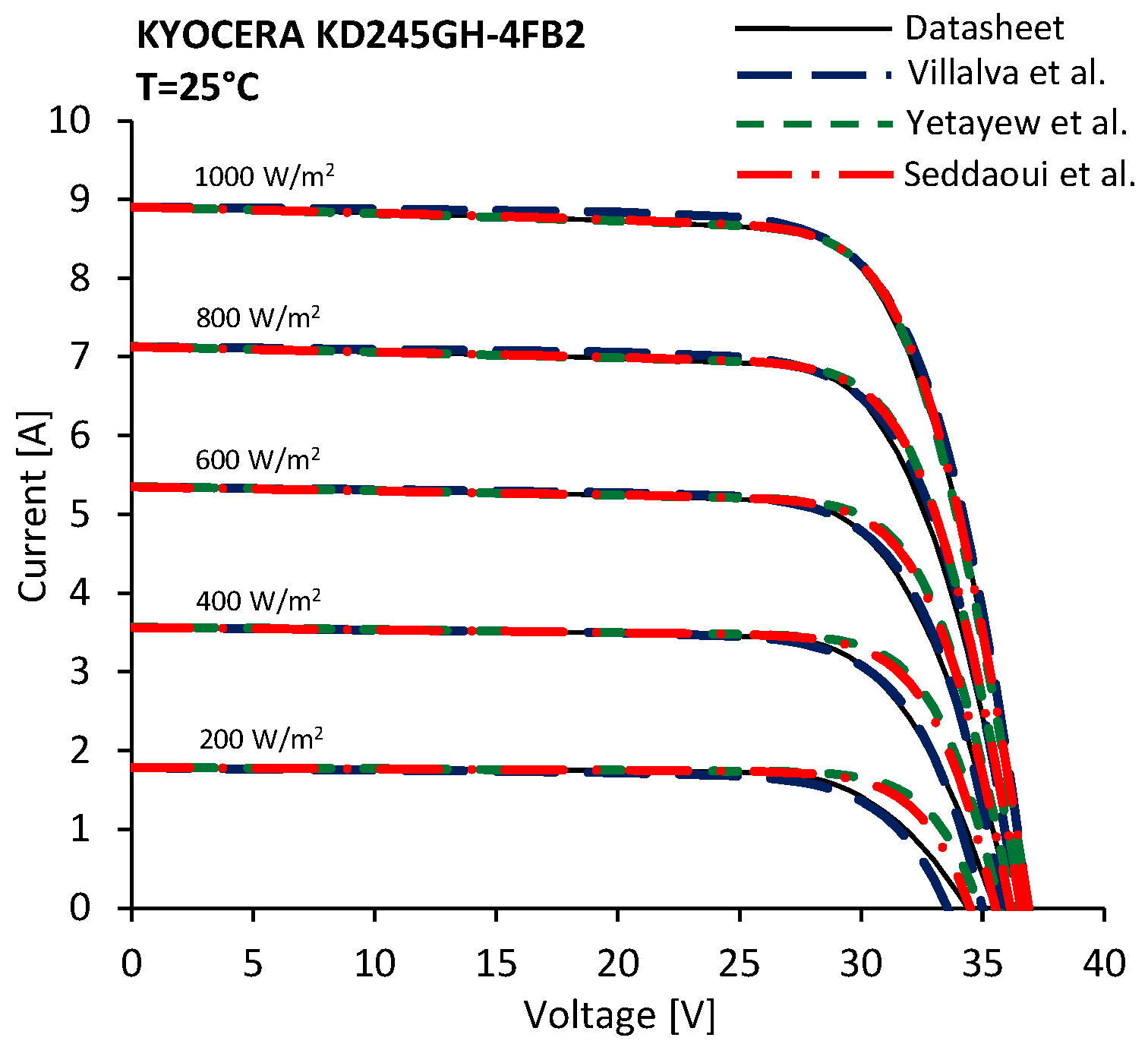
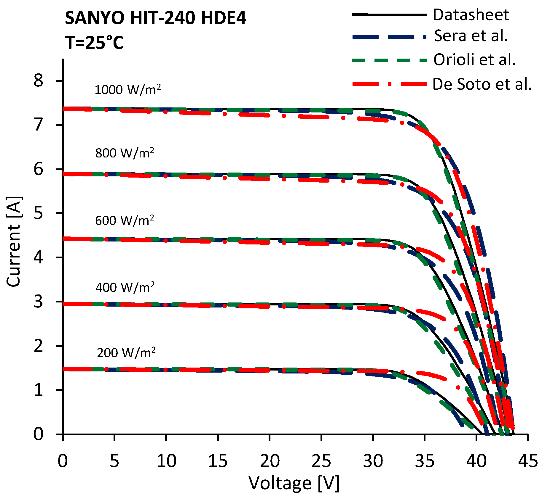
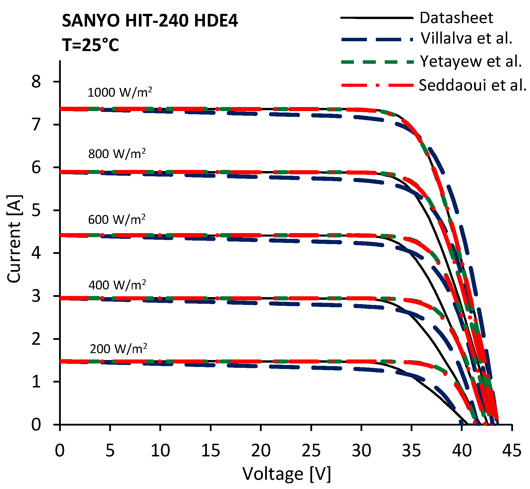
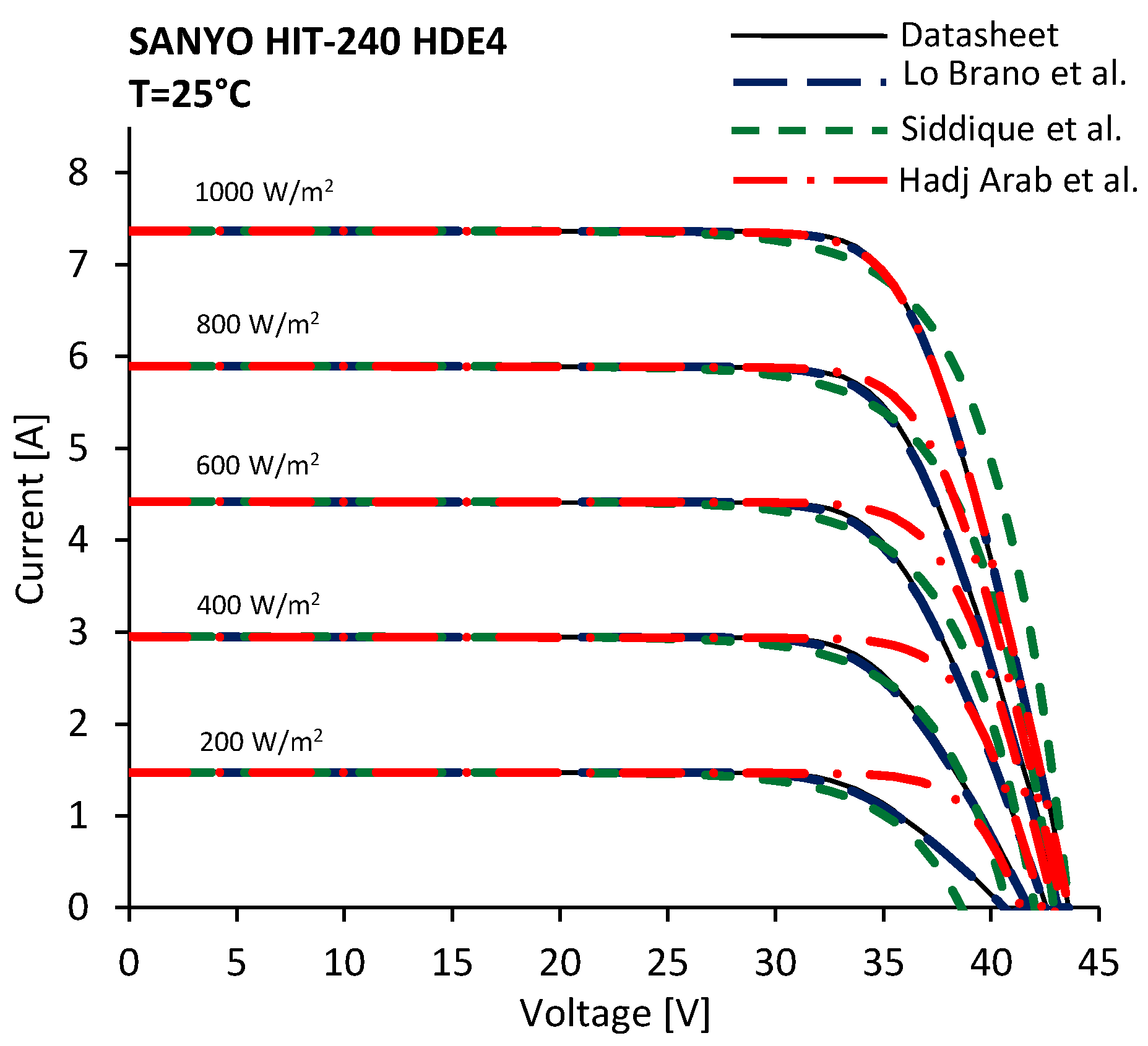
In order to assess the accuracy of the proposed procedures, a comparison between the tested one-diode models was made using the I-V characteristics extracted from manufacturer datasheets by reading the coordinates of a large number of points on each curve. For the sake of brevity, only two PV modules, based on different production technologies, were considered. Obviously, because the results are strongly affected by the particular shape of the considered I-V characteristics, a more reliable assessment may require the use of a greater number of PV modules. Actually, the aim of this accuracy assessment is not ranking the best or the worst among the analysed models, but only reckoning the range of predictable precision in order to calibrate the proposed criterion. The data of the simulated PV modules are listed in

Table 2. Performance data of the simulated PV panels.

PANEL	Type	Ncs	Voc,ref [V]	Isc,ref [A]	Vmp,ref [V]	Imp,ref [A]	μV,oc [V/°C]	μI,sc [A/°C]	Rso [Ω]	Rsho [Ω]
Kyocera KD245GH-4FB2	Poly	60	36.90	8.91	29.80	8.23	−1.33 × 10−1	5.35 × 10−3	0.493	120.5
Sanyo HIT-240 HDE4	HIT	60	43.60	7.37	35.50	6.77	−1.09 × 10−1	2.21 × 10−3	0.873	3204.6

.

The Lo Brano et al. and the Orioli et al. models also use the open voltage at G = 200 W/m² and T = 25 °C, which are 34.40 V and 40.61 V per the Kyocera and the Sanyo PV modules, respectively. To calculate parameter K, these models use the values of voltage and current at the MPP for G = 1000 W/m² and T = 75 °C, which are 22.50 V and 8.35 A, for the Kyocera PV panel, and 28.89 V and 7.13 A, for the Sanyo PV module. In order to get a reliable comparison between the calculated and the experimental data, numerous points were extracted from the I-V characteristics issued by the manufacturer, considering both the constant solar irradiance and the constant cell temperature curves. To calculate R_sho and R_so, the reciprocal of slopes of the I-V curve in correspondence of the short circuit and open circuit points were extracted from the issued I-V characteristics following the graphical procedure described in [44].

Table 3. Model parameters of Kyocera KD245GH-4FB2 at the SRC.

Model	IL,ref [A]	I0,ref [A]	n [V/K]	Rs [Ω]	Rsh [Ω]	K [Ω/°C]
Hadj Arab et al.	8.9336	1.6881 × 10−10	5.0199 × 10−3	0.3189	120.4800	-
De Soto et al.	8.9270	1.5328 × 10−9	5.5111 × 10−3	0.2854	149.2274	-
Sera et al.	8.9126	3.9061 × 10−7	7.3079 × 10−3	0.1615	548.4865	-
Villalva et al.	8.9157	8.9791 × 10−8	6.7215 × 10−3	0.2000	311.0804	-
Lo Brano et al.	8.9337	1.6143 × 10−10	5.0103 × 10−3	0.3200	120.1600	8.6230 × 10−4
Seddaoui et al.	8.9336	1.6881 × 10−10	5.0199 × 10−3	0.3189	120.4800	-
Siddique et al.	8.9100	5.6501 × 10−5	2.7675 × 10−4	0.1181	3.7815·106	-
Yetayew et al.	8.9384	2.0052 × 10−11	4.6206 × 10−3	0.3552	111.6164	-
Orioli et al.	8.9100	1.6965 × 10−9	5.5369 × 10−3	0.2722	142.8660	9.7323 × 10−4

and

Table 4. Model parameters of Sanyo HIT-240 HDE4 at the SRC.

MODEL	IL,ref [A]	I0,ref [A]	n [V/K]	Rs [Ω]	Rsh [Ω]	K [Ω/°C]
Hadj Arab et al.	7.3716	9.6843 × 10−14	4.5754 × 10−3	0.6877	3204.6400	-
De Soto et al.	7.3958	1.8862 × 10−11	5.4876 × 10−3	0.4555	130.0439	-
Sera et al.	7.3721	7.9253 × 10−7	9.1206 × 10−3	0.1420	488.0935	-
Villalva et al.	7.3842	2.6233 × 10−9	6.7215 × 10−3	0.3300	171.2005	-
Lo Brano et al.	7.3716	9.6380 × 10−14	4.5747 × 10−3	0.6877	3203.9523	−1.600 × 103
Seddaoui et al.	7.3716	9.6843 × 10−14	4.5754 × 10−3	0.6877	3204.6400	-
Siddique et al.	7.3700	5.3195 × 10−6	7.1635 × 10−3	0.0542	2.2747·107	-
Yetayew et al.	7.3716	1.5551 × 10−14	4.3277 × 10−3	0.7152	3212.5368	-
Orioli et al.	7.3700	3.6671 × 10−19	3.2907 × 10−3	0.8200	736.4149	−6.4618 × 104

list the values of the parameters evaluated with the analysed models.

The values of Table 3 and Table 4 were used to calculate the I-V characteristics of the selected PV panels. In Figure 4, Figure 5, Figure 6, Figure 7, Figure 8 and Figure 9 the I-V curves evaluated at T = 25 °C with the models of Hadj Arab et al., De Soto et al., Sera et al., Villalva et al., Lo Brano et al., Seddaoui et al., Siddique et al., Yetayew et al. and Orioli et al. are compared with the characteristics issued by manufacturers.

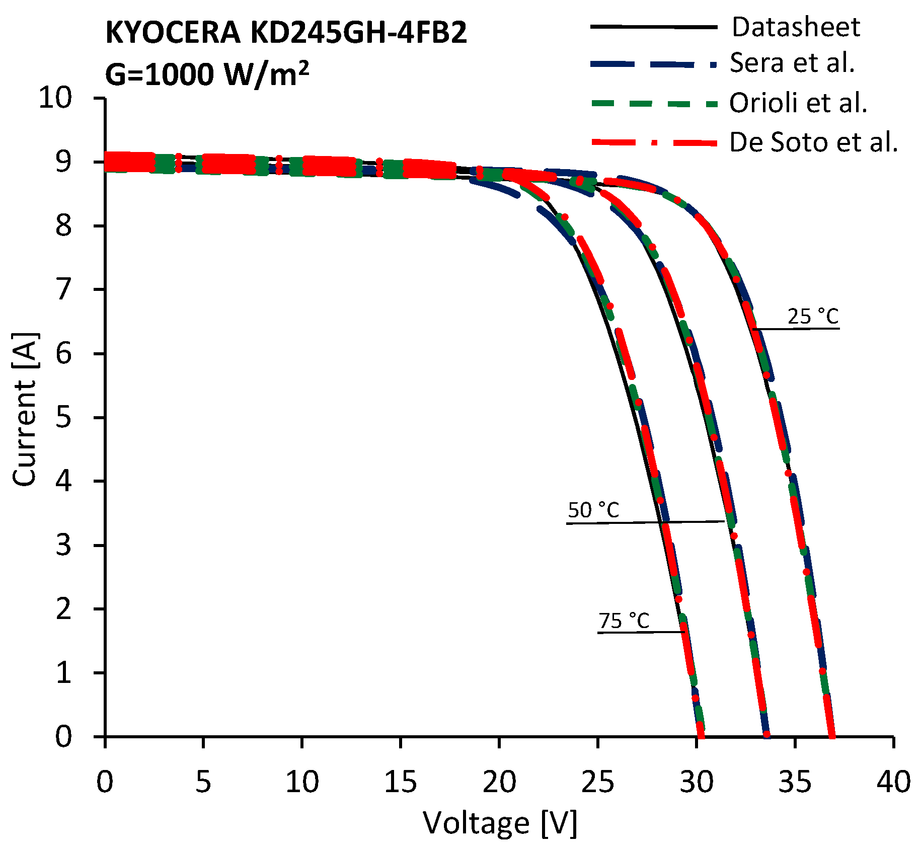
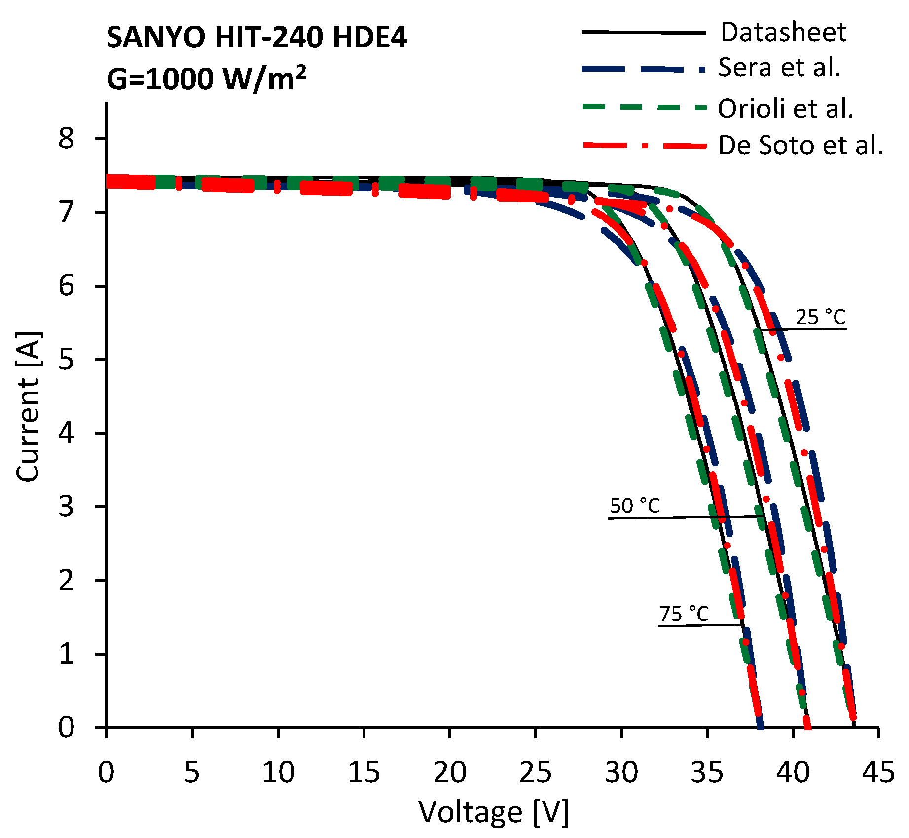
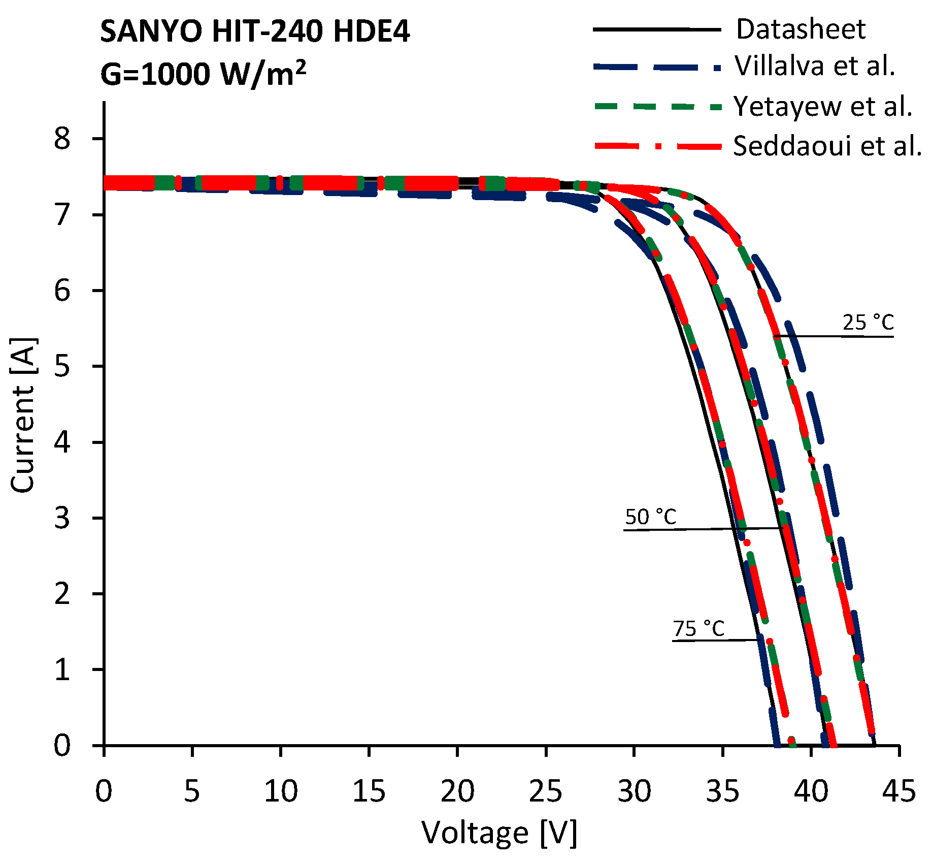
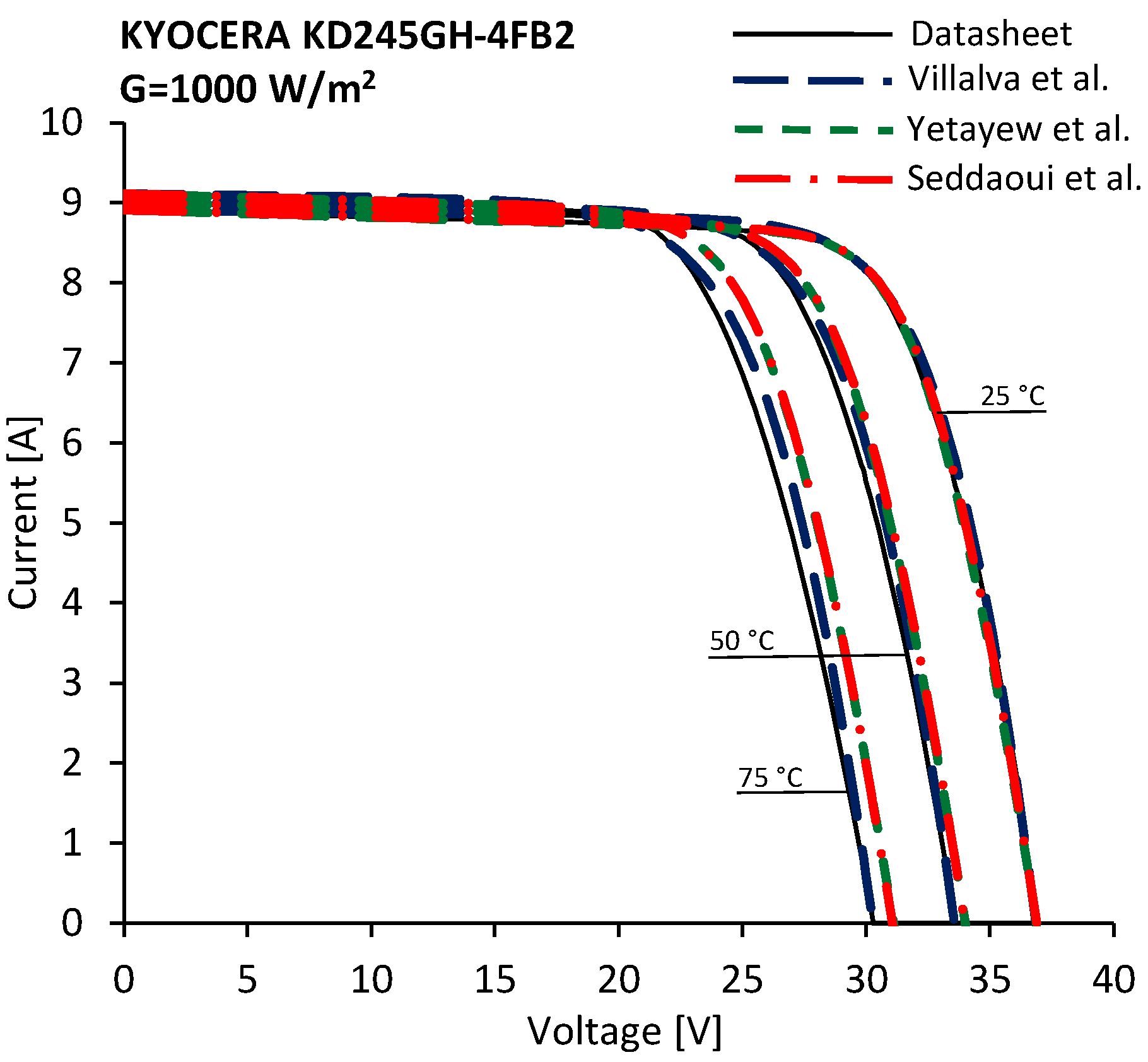
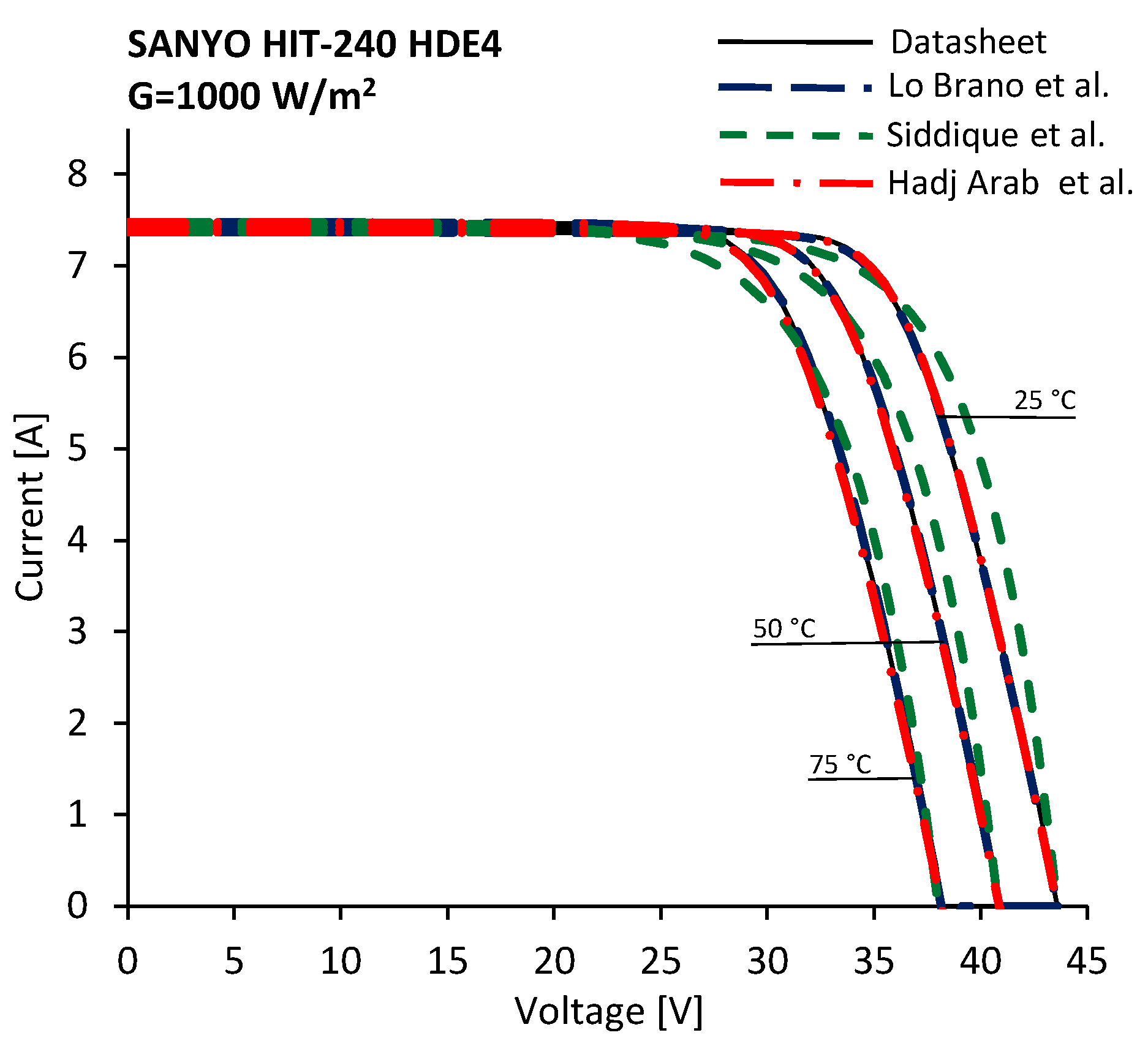
Because the Hadj Arab et al. and the Seddaoui et al. are based on the same information, it is not surprising that the I-V curves at the SRC resulted quite similar. Conversely, significant differences are expected for values of solar irradiance and temperature different from the SRC. Figure 10, Figure 11, Figure 12, Figure 13, Figure 14 and Figure 15 depict the I-V curves evaluated at G = 1000 W/m² and the characteristics issued by manufacturers.

It can be generally observed in Figure 4, Figure 5, Figure 6, Figure 7, Figure 8, Figure 9, Figure 10, Figure 11, Figure 12, Figure 13, Figure 14 and Figure 15 that most of the models result less accurate for values of voltage greater than the MPP voltage. Moreover, it can be inferred that the one-diode models are more precise if they are used to evaluate the I-V characteristics of the Kyocera PV panel. This occurrence may be due to the different shape of the I-V curves used to compare the analysed models. It can be also observed that models that use similar values of the parameters listed in Table 3 and Table 4 yield different I-V curves for values of the solar irradiance and the cell temperature far from the SRC because different approaches were adopted to describe the effects of the solar irradiance and cell temperature. To quantify the accuracy of the analysed models, the mean absolute difference (MAD) for current and power was calculated with the following expressions:

$$\mathrm{MAD}(I)=\frac{1}{N}{\displaystyle \sum _{j=1}^N\left|I_{calc,j}-I_{iss,j}\right|}$$

(11)

$$\mathrm{MAD}(P)=\frac{1}{N}{\displaystyle \sum _{j=1}^N\left|V_{iss,j}{I}_{calc,j}-V_{iss,j}{I}_{iss,j}\right|}$$

(12)

in which V_iss,j and I_iss,j are the voltage and current of the j-th point extracted from the I-V characteristics issued by manufacturers, I_calc,j is the value of the current calculated in correspondence of V_iss,j and N is the number of extracted points. Moreover, in order to assess the range of dispersion of the results, also the maximum difference (MD) for current and power was evaluated using the following relations:

$$\mathrm{MD}(I)=\mathrm{MAX}\left[I_{calc,j}-I_{iss,j}\right]$$

(13)

$$\mathrm{MD}(P)=\mathrm{MAX}\left[V_{iss,j}{I}_{calc,j}-V_{iss,j}{I}_{iss,j}\right]$$

(14)

Table 5. Mean absolute current and power differences between the calculated and the issued I–V characteristics at temperature T = 25 °C.

PV Panel	Mad		Irradiance [W/m2]
			200	400	600	800	1000
Kyocera KD245GH-4FB2	Current [A]	Hadj Arab et al. model	0.110	0.153	0.130	0.111	0.042
		De Soto et al. model	0.101	0.149	0.132	0.124	0.052
		Sera et al. model	0.094	0.065	0.057	0.092	0.136
		Villalva et al. model	0.077	0.054	0.050	0.089	0.104
		Lo Brano et al. model	0.041	0.059	0.082	0.033	0.042
		Seddaoui et al. model	0.138	0.187	0.156	0.131	0.042
		Siddique et al. model	0.137	0.123	0.087	0.094	0.166
		Yetayew et al. model	0.209	0.253	0.192	0.136	0.051
		Orioli et al. model	0.076	0.107	0.115	0.042	0.064
	Power [W]	Hadj Arab et al. model	3.138	4.718	4.077	3.595	1.350
		De Soto et al. model	3.103	4.681	4.166	3.948	1.608
		Sera et al. model	2.851	2.075	1.772	2.869	4.257
		Villalva et al. model	2.299	1.769	1.607	2.805	3.192
		Lo Brano et al. model	1.246	1.870	2.698	1.074	1.356
		Seddaoui et al. model	4.320	5.977	5.006	4.216	1.350
		Siddique et al. model	4.173	3.901	2.698	2.881	5.229
		Yetayew et al. model	6.625	8.123	6.184	4.387	6.625
		Orioli et al. model	2.313	3.421	3.738	1.366	2.044
Sanyo HIT-240 HDE4	Current [A]	Hadj Arab et al. model	0.230	0.324	0.323	0.186	0.021
		De Soto et al. model	0.173	0.286	0.333	0.307	0.242
		Sera et al. model	0.072	0.100	0.174	0.234	0.321
		Villalva et al. model	0.109	0.194	0.266	0.269	0.267
		Lo Brano et al. model	0.015	0.028	0.022	0.041	0.021
		Seddaoui et al. model	0.235	0.327	0.326	0.187	0.021
		Siddique et al. model	0.102	0.074	0.136	0.212	0.337
		Yetayew et al. model	0.251	0.346	0.340	0.190	0.024
		Orioli et al. model	0.056	0.079	0.075	0.100	0.078
	Power [W]	Hadj Arab et al. model	8.656	12.436	12.518	7.226	0.828
		De Soto et al. model	6.362	10.750	12.598	11.382	8.686
		Sera et al. model	2.303	3.465	6.428	8.855	12.496
		Villalva et al. model	3.303	6.735	9.664	9.858	9.846
		Lo Brano et al. model	0.487	1.011	0.794	1.601	0.830
		Seddaoui et al. model	8.813	12.551	12.593	7.256	0.828
		Siddique et al. model	3.591	2.646	5.060	8.179	13.321
		Yetayew et al. model	9.427	13.281	13.125	7.350	0.963
		Orioli et al. model	1.963	2.913	2.805	3.799	2.952

and

Table 6. Mean absolute current and power differences between the calculated andthe issued I–V characteristics at irradiance G = 1000 W/m².

PV Panel	Mad		Temperature [°C]
			25	50	75
Kyocera KD245GH-4FB2	Current [A]	Hadj Arab et al. model	0.042	0.125	0.200
		De Soto et al. model	0.052	0.116	0.136
		Sera et al. model	0.136	0.150	0.212
		Villalva et al. model	0.104	0.178	0.191
		Lo Brano et al. model	0.042	0.048	0.063
		Seddaoui et al. model	0.042	0.314	0.655
		Siddique et al. model	0.166	0.308	0.413
		Yetayew et al. model	0.051	0.287	0.651
		Orioli et al. model	0.064	0.088	0.113
	Power [W]	Hadj Arab et al. model	1.350	3.628	5.215
		De Soto et al. model	1.608	3.269	3.481
		Sera et al. model	4.257	4.298	4.858
		Villalva et al. model	3.192	4.960	4.943
		Lo Brano et al. model	1.356	1.333	1.611
		Seddaoui et al. model	1.350	9.453	18.222
		Siddique et al. model	5.229	8.807	11.297
		Yetayew et al. model	6.625	8.680	18.140
		Orioli et al. model	2.044	2.526	2.984
Sanyo HIT-240 HDE4	Current [A]	Hadj Arab et al. model	0.021	0.035	0.066
		De Soto et al. model	0.242	0.205	0.151
		Sera et al. model	0.321	0.292	0.273
		Villalva et al. model	0.267	0.236	0.195
		Lo Brano et al. model	0.021	0.029	0.034
		Seddaoui et al. model	0.021	0.114	0.247
		Siddique et al. model	0.337	0.283	0.231
		Yetayew et al. model	0.024	0.107	0.252
		Orioli et al. model	0.078	0.102	0.117
	Power [W]	Hadj Arab et al. model	0.828	1.292	2.257
		De Soto et al. model	8.686	6.729	4.506
		Sera et al. model	12.496	9.984	8.167
		Villalva et al. model	9.846	8.019	6.132
		Lo Brano et al. model	0.830	1.049	1.142
		Seddaoui et al. model	0.828	4.270	8.799
		Siddique et al. model	13.321	10.170	7.550
		Yetayew et al. model	0.963	4.042	8.991
		Orioli et al. model	2.952	3.623	3.951

list the MAD(I)s and MAD(P)s for the Kyocera KD245GH-4FB2 and Sanyo HIT-240 HDE4 PV panels.

Considering the solar irradiance variation, if the Hadj Arab et al., the Villalva et al., the Lo Brano et al. and the Seddaoui et al. models are used for the Kyocera PV panel, MAD(I)s ranging from 0.041 A to 0.054 A can be obtained. In the same conditions, the MAD(P)s vary from 1.074 W to 1.769 W. For the Sanyo PV module, the smallest MAD(I)s, which occur when the Hadj Arab et al., the Lo Brano et al. and the Seddaoui et al. models are used, vary between 0.015 A and 0.041 A. The smallest MAD(P)s derived from the same models. These differences vary between 0.487 W and 1.601 W. The greatest MAD(I)s for the Kyocera PV panel, which are calculated with the Siddique et al. and the Yetayew et al. models, vary from 0.136 A to 0.253 A. The Yetayew et al. model yields the greatest MAD(P)s, which range from 4.387 W to 8.123 W. For the Sanyo PV module, the greatest MAD(I)s are noted for the De Soto et al., the Siddique et al. and the Yetayew et al. models. These differences are contained in the range from 0.251 A to 0.346 A. The greatest MAD(P)s, which belong to the same models, vary from 9.427 W to 13.321 W.

At constant solar irradiance, if the Hadj Arab et al., the Lo Brano et al. and the Seddaoui et al. models are used for the Kyocera PV panel, MAD(I)s ranging from 0.042 A to 0.063 A can be observed. In the same conditions, the MAD(P)s vary from 1.333 W to 1.611 W. For the Sanyo PV module, the smallest MAD(I)s, which are obtained from the Hadj Arab et al., the Lo Brano et al. and the Seddaoui et al. models, vary between 0.021 A and 0.034 A. The smallest mean power differences are obtained from the same models. These differences vary between 0.828 W and 1.142 W. For the Kyocera PV module, the greatest MAD(I)s are generated by the Seddaoui et al. and the Siddique et al. models. These differences are contained in the range from 0.166 A to 0.655 A. The greatest MAD(P)s, which are obtained from the Seddaoui et al. and the Yetayew et al. models, vary between 6.625 W and 18.222 W. The greatest MAD(I)s for the Sanyo PV panel, which are obtained from the Sera et al. and the Siddique et al. models, vary from 0.273 A to 0.337 A. The Siddique et al. and the Yetayew et al. models yield the greatest MAD(P)s, which range from 8.991 W to 13.321 W of the issued rated maximum power. In

Table 7. Maximum current differences between the calculated and the issued I-V characteristics of Kyocera KD245GH-4FB2, at temperature T = 25 °C.

Parameters At The Maximum Difference Points		Irradiance [W/m2]
		200	400	600	800	1000
Hadj Arab et al. model	Voltage [V]	33.0	33.0	33.0	32.5	32.5
	Issued Current [A]	0.603	1.896	3.335	5.093	6.596
	Calculated Current [A]	0.849	2.306	3.708	5.428	6.735
	Difference [A]	0.246	0.410	0.373	0.335	0.139
De Soto et al. model	Voltage [V]	32.0	32.5	33.0	32.5	32.5
	Issued Current [A]	0.948	2.165	3.335	5.093	6.596
	Calculated Current [A]	1.200	2.553	3.686	5.428	6.765
	Difference [A]	0.252	0.388	0.351	0.335	0.169
Sera et al. model	Voltage [V]	33.0	34.5	35.5	33.5	34.5
	Issued Current [A]	0.603	0.843	0.891	4.224	4.305
	Calculated Current [A]	0.221	0.460	0.466	4.479	4.687
	Difference [A]	−0.382	−0.383	−0.425	0.255	0.382
Villalva et al. model	Voltage [V]	33.5	35.0	35.5	33.5	34.0
	Issued Current [A]	0.394	0.429	0.891	4.224	4.992
	Calculated Current [A]	0.037	0.001	0.553	4.471	5.259
	Difference [A]	−0.357	−0.428	−0.338	0.247	0.267
Lo Brano et al. model	Voltage [V]	32.0	33.5	34.4	35.0	32.5
	Issued Current [A]	0.948	1.591	2.151	2.441	6.596
	Calculated Current [A]	0.860	1.443	1.894	2.325	6.728
	Difference [A]	−0.088	−0.148	−0.257	−0.116	0.132
Seddaoui et al. model	Voltage [V]	32.5	33.0	33.0	32.5	32.5
	Issued Current [A]	0.780	1.896	3.335	5.093	6.596
	Calculated Current [A]	1.145	2.395	3.765	5.460	6.735
	Difference [A]	0.366	0.499	0.430	0.367	0.139
Siddique et al. model	Voltage [V]	33.0	34.5	35.5	36.2	34.5
	Issued Current [A]	0.603	0.843	0.891	0.655	4.305
	Calculated Current [A]	0.045	0.267	0.317	0.365	4.786
	Difference [A]	−0.558	−0.576	−0.574	−0.290	0.481
Yetayew et al. model	Voltage [V]	33.0	33.0	33.0	32.5	36.2
	Issued Current [A]	0.603	1.896	3.335	5.093	1.500
	Calculated Current [A]	1.144	2.532	3.844	5.471	1.324
	Difference [A]	0.541	0.636	0.509	0.378	−0.176
Orioli et al. model	Voltage [V]	33.0	34.4	35.5	36.2	32.5
	Issued Current [A]	0.603	0.945	0.891	0.655	6.596
	Calculated Current [A]	0.450	0.674	0.536	0.444	6.816
	Difference [A]	−0.153	−0.271	−0.355	−0.211	0.220

and

Table 8. Maximum current differences between the calculated and the issued I-V characteristics of Sanyo HIT-240 HDE4, at temperature T = 25 °C.

Parameters At The Maximum Difference Points		Irradiance [W/m2]
		200	400	600	800	1000
Hadj Arab et al. model	Voltage [V]	38.5	39.1	39.1	39.1	42.7
	Issued Current [A]	0.471	1.187	2.171	3.350	1.070
	Calculated Current [A]	1.147	2.128	3.093	3.903	0.971
	Difference [A]	0.676	0.941	0.922	0.553	−0.099
De Soto et al. model	Voltage [V]	38.5	39.1	39.7	39.1	39.7
	Issued Current [A]	0.471	1.187	1.819	3.350	4.018
	Calculated Current [A]	1.000	2.029	2.802	4.191	4.653
	Difference [A]	0.529	0.842	0.983	0.841	0.635
Sera et al. model	Voltage [V]	38.5	40.9	39.1	40.3	40.3
	Issued Current [A]	0.471	0.401	2.171	2.458	3.485
	Calculated Current [A]	0.254	0.117	2.722	3.224	4.516
	Difference [A]	−0.217	−0.284	0.551	0.766	1.031
Villalva et al. model	Voltage [V]	29.8	38.5	39.1	39.7	39.7
	Issued Current [A]	1.464	1.414	2.171	2.934	4.018
	Calculated Current [A]	1.291	1.922	2.918	3.702	4.791
	Difference [A]	−0.173	0.508	0.747	0.768	0.773
Lo Brano et al. model	Voltage [V]	34.9	34.9	34.3	42.1	42.7
	Issued Current [A]	1.144	2.551	4.128	1.010	1.070
	Calculated Current [A]	1.104	2.491	4.080	0.863	0.971
	Difference [A]	−0.040	−0.060	−0.048	−0.147	−0.099
Seddaoui et al. model	Voltage [V]	38.5	39.1	39.1	39.1	42.7
	Issued Current [A]	0.471	1.187	2.171	3.350	1.070
	Calculated Current [A]	1.152	2.132	3.095	3.904	0.971
	Difference [A]	0.681	0.945	0.924	0.554	−0.099
Siddique et al. model	Voltage [V]	38.5	40.6	39.1	40.3	40.6
	Issued Current [A]	0.471	0.554	2.171	2.458	3.233
	Calculated Current [A]	0.051	0.150	2.613	3.195	4.358
	Difference [A]	−0.420	−0.404	0.442	0.737	1.125
Yetayew et al. model	Voltage [V]	38.5	39.1	39.1	39.1	42.7
	Issued Current [A]	0.471	1.187	2.171	3.350	1.070
	Calculated Current [A]	1.195	2.177	3.121	3.896	0.953
	Difference [A]	0.724	0.990	0.950	0.546	−0.117
Orioli et al. model	Voltage [V]	37.3	37.3	38.5	39.7	40.9
	Issued Current [A]	0.720	1.865	2.508	2.934	2.923
	Calculated Current [A]	0.600	1.682	2.326	2.682	2.701
	Difference [A]	−0.120	−0.183	−0.182	−0.252	−0.222

the values of MD(I) and MD(P) for the analysed panels, calculated considering the I-V curves at a constant cell temperature of 25 °C, are listed.

Considering the I-V curves at constant temperature for the Kyocera PV panel, the Lo Brano et al. model seems to be the most accurate; the MD(I)s vary from −0.257 A to 0.132 A. The greatest current differences, which are contained in the range −0.574 A to 0.636 A, are observed for the Siddique et al. and the Yetayew et al. models. The smallest MD(I)s are obtained for the Sanyo PV module from the Hadj Arab et al., the Lo Brano et al. and the Seddaoui et al. models; these differences are in the range −0.040 A to −0.147 A. The greatest inaccuracies derive from the de Soto et al., the Siddique et al. and the Yetayew et al. models. For these models differences varying between 0.724 A and 1.125 A were calculated.

Table 9. Maximum current differences between the calculated and the issued I-V characteristics of Kyocera KD245GH-4FB2, at irradiance G = 1000 W/m².

Parameters at the Maximum Difference Points		Temperature [°C]
		25	50	75
Hadj Arab et al. model	Voltage [V]	32.5	29.5	26.0
	Issued Current [A]	6.596	6.039	5.950
	Calculated Current [A]	6.735	6.421	6.594
	Difference [A]	0.139	0.382	0.644
De Soto et al. model	Voltage [V]	32.5	29.5	26.0
	Issued Current [A]	6.596	6.039	5.950
	Calculated Current [A]	6.765	6.362	6.412
	Difference [A]	0.169	0.323	0.462
Sera et al. model	Voltage [V]	34.5	31.0	27.5
	Issued Current [A]	4.305	4.278	4.241
	Calculated Current [A]	4.687	4.738	4.778
	Difference [A]	0.382	0.460	0.537
Villalva et al. model	Voltage [V]	34.0	31.0	27.5
	Issued Current [A]	4.992	4.278	4.241
	Calculated Current [A]	5.259	4.743	4.886
	Difference [A]	0.267	0.465	0.645
Lo Brano et al. model	Voltage [V]	32.5	29.0	26.0
	Issued Current [A]	6.596	6.515	5.950
	Calculated Current [A]	6.728	6.683	6.173
	Difference [A]	0.132	0.168	0.223
Seddaoui et al. model	Voltage [V]	32.5	31.0	29.0
	Issued Current [A]	6.596	4.278	2.122
	Calculated Current [A]	6.735	5.063	3.638
	Difference [A]	0.139	0.785	1.516
Siddique et al. model	Voltage [V]	34.5	31.0	28.5
	Issued Current [A]	4.305	4.278	2.875
	Calculated Current [A]	4.786	5.111	4.012
	Difference [A]	0.481	0.833	1.137
Yetayew et al. model	Voltage [V]	36.2	33.6	29.5
	Issued Current [A]	1.500	0.000	1.326
	Calculated Current [A]	1.324	0.787	2.822
	Difference [A]	−0.176	0.787	1.496
Orioli et al. model	Voltage [V]	32.5	29.5	27.5
	Issued Current [A]	6.596	6.039	4.241
	Calculated Current [A]	6.816	6.300	4.562
	Difference [A]	0.220	0.261	0.321

and

Table 10. Maximum current differences between the calculated and the issued I-V characteristics of Sanyo HIT-240 HDE4, at irradiance G = 1000 W/m².

Parameters at the Maximum Difference Points		Temperature [°C]
		25	50	75
Hadj Arab et al. model	Voltage [V]	42.7	39.7	37.3
	Issued Current [A]	1.070	1.440	1.120
	Calculated Current [A]	0.971	1.293	0.951
	Difference [A]	−0.099	−0.147	−0.169
De Soto et al. model	Voltage [V]	39.7	37.3	34.3
	Issued Current [A]	4.018	3.810	4.100
	Calculated Current [A]	4.653	4.263	4.403
	Difference [A]	0.635	0.453	0.303
Sera et al. model	Voltage [V]	40.3	38.2	35.5
	Issued Current [A]	3.485	2.981	2.984
	Calculated Current [A]	4.516	3.789	3.535
	Difference [A]	1.031	0.808	0.551
Villalva et al. model	Voltage [V]	39.7	37.3	34.3
	Issued Current [A]	4.018	3.810	4.100
	Calculated Current [A]	4.791	4.409	4.556
	Difference [A]	0.773	0.599	0.456
Lo Brano et al. model	Voltage [V]	42.7	40.6	37.9
	Issued Current [A]	1.070	0.455	0.438
	Calculated Current [A]	0.971	0.325	0.293
	Difference [A]	−0.099	−0.130	−0.145
Seddaoui et al. model	Voltage [V]	42.7	40.9	38.2
	Issued Current [A]	1.070	0.000	0.000
	Calculated Current [A]	0.971	0.383	0.832
	Difference [A]	−0.099	0.383	0.832
Siddique et al. model	Voltage [V]	40.6	38.2	35.5
	Issued Current [A]	3.233	2.981	2.984
	Calculated Current [A]	4.358	3.871	3.542
	Difference [A]	1.125	0.890	0.558
Yetayew et al. model	Voltage [V]	42.7	40.9	38.2
	Issued Current [A]	1.070	0.000	0.000
	Calculated Current [A]	0.953	0.396	0.858
	Difference [A]	−0.117	0.396	0.858
Orioli et al. model	Voltage [V]	40.9	36.7	34.9
	Issued Current [A]	2.923	4.358	3.589
	Calculated Current [A]	2.701	4.109	3.295
	Difference [A]	−0.222	−0.249	−0.294

list the MD(I)s calculated for Kyocera KD245GH-4FB2 and Sanyo HIT-240 HDE4 PV panels at a constant solar irradiance of 1000 W/m².

The smallest MD(I)s for the Kyocera PV module at constant solar irradiance arise from the Lo Brano et al. model. Such differences range from 0.132 A to 0.223 A. The greatest inaccuracies are provided by the Seddaoui et al. and the Siddique et al. models, for which differences varying between 0.481 A and 1.516 A are observed. The Hadj Arab et al., the Lo Brano et al. and the Seddaoui et al. model seem to be the most accurate for the Sanyo PV panel; the MD(I)s vary from −0.099 A to −0.145 A. The greatest current differences, which are contained in the range 0.858 A to 1.125 A, are observed for the Siddique et al. and the Yetayew et al. models.

Table 11. Maximum power differences between the calculated and the issued I-V characteristics of Kyocera KD245GH-4FB2, at temperature T = 25 °C.

Parameters at the Maximum Difference Points		Irradiance [W/m2]
		200	400	600	800	1000
Hadj Arab et al. model	Voltage [V]	33.0	33.5	33.0	32.5	32.5
	Issued Power [W]	19.91	53.31	110.06	165.51	214.37
	Calculated Power [W]	28.02	67.00	122.36	176.41	218.90
	Difference [W]	8.11	13.69	12.30	10.90	4.53
De Soto et al. model	Voltage [V]	32.5	33.0	33.0	32.5	32.5
	Issued Power [W]	25.34	62.55	110.06	165.51	214.37
	Calculated Power [W]	33.44	75.23	121.63	176.41	219.88
	Difference [W]	8.10	12.68	11.57	10.90	5.51
Sera et al. model	Voltage [V]	33.0	34.5	35.5	34.0	34.5
	Issued Power [W]	19.91	29.07	31.65	125.37	148.52
	Calculated Power [W]	7.29	15.85	16.56	133.90	161.71
	Difference [W]	−12.62	−13.22	−15.09	8.53	13.19
Villalva et al. model	Voltage [V]	33.5	35.0	35.5	33.5	34.0
	Issued Power [W]	13.20	15.00	31.65	141.51	169.73
	Calculated Power [W]	1.24	0.05	19.62	149.76	178.81
	Difference [W]	−11.96	−14.95	−12.03	8.25	9.08
Lo Brano et al. model	Voltage [V]	32.0	33.5	34.4	35.0	36.2
	Issued Power [W]	30.34	53.31	74.00	85.42	54.30
	Calculated Power [W]	27.52	48.33	65.17	81.38	49.86
	Difference [W]	−2.82	−4.98	−8.83	−4.04	-4.44
Seddaoui et al. model	Voltage [V]	32.5	33.0	33.0	32.5	32.5
	Issued Power [W]	25.34	62.55	110.06	165.51	214.37
	Calculated Power [W]	37.23	79.04	124.26	177.43	218.90
	Difference [W]	11.89	16.49	14.20	11.92	4.53
Siddique et al. model	Voltage [V]	33.0	34.5	35.5	36.2	34.5
	Issued Power [W]	19.91	29.07	31.65	23.70	148.52
	Calculated Power [W]	1.49	9.23	11.25	13.21	165.12
	Difference [W]	−18.42	−19.84	−20.40	−10.49	16.60
Yetayew et al. model	Voltage [V]	33.0	33.5	33.0	32.5	32.5
	Issued Power [W]	13.20	53.31	110.06	165.51	54.30
	Calculated Power [W]	31.20	74.63	126.84	177.79	47.92
	Difference [W]	18.00	21.32	16.78	12.28	−6.38
Orioli et al. model	Voltage [V]	33.0	34.4	35.5	36.2	32.5
	Issued Power [W]	19.91	32.52	31.65	23.70	214.37
	Calculated Power [W]	14.85	23.17	19.04	16.09	221.53
	Difference [W]	−5.06	−9.35	−12.61	−7.61	7.16

,

Table 12. Maximum power differences between the calculated and the issued I-V characteristics of Sanyo HIT-240 HDE4, at temperature T = 25 °C.

Parameters at the Maximum Difference Points		Irradiance [W/m2]
		200	400	600	800	1000
Hadj Arab et al. model	Voltage [V]	39.1	39.1	39.1	39.1	42.7
	Issued Power [W]	13.28	46.44	84.96	131.07	45.73
	Calculated Power [W]	39.34	83.25	121.03	152.70	41.51
	Difference [W]	26.06	36.81	36.07	21.63	−4.22
De Soto et al. model	Voltage [V]	38.5	39.1	39.7	39.7	39.7
	Issued Power [W]	18.13	46.44	72.26	116.58	159.62
	Calculated Power [W]	38.53	79.38	111.34	149.71	184.86
	Difference [W]	20.40	32.94	39.08	33.13	25.24
Sera et al. model	Voltage [V]	38.5	40.9	39.1	40.3	40.6
	Issued Power [W]	18.13	16.42	84.96	99.14	131.28
	Calculated Power [W]	9.78	4.77	106.49	130.01	173.06
	Difference [W]	−8.35	−11.65	21.53	30.87	41.78
Villalva et al. model	Voltage [V]	37.3	38.5	39.7	40.3	39.7
	Issued Power [W]	26.89	54.47	72.26	99.14	159.62
	Calculated Power [W]	33.02	74.04	101.86	129.68	190.36
	Difference [W]	6.13	19.57	29.60	30.54	30.74
Lo Brano et al. model	Voltage [V]	34.9	34.9	42.1	42.1	42.7
	Issued Power [W]	39.96	89.08	12.36	42.57	45.73
	Calculated Power [W]	38.55	86.97	10.54	36.38	41.49
	Difference [W]	−1.41	−2.11	−1.82	−6.19	−4.24
Seddaoui et al. model	Voltage [V]	38.5	39.1	39.1	39.1	42.7
	Issued Power [W]	18.13	46.44	84.96	131.07	45.73
	Calculated Power [W]	44.39	83.41	121.09	152.74	41.51
	Difference [W]	26.26	36.97	36.13	21.67	−4.22
Siddique et al. model	Voltage [V]	38.5	40.6	39.1	40.3	40.6
	Issued Power [W]	18.13	22.48	84.96	99.14	131.28
	Calculated Power [W]	1.96	6.07	102.25	128.85	176.96
	Difference [W]	−16.17	−16.41	17.29	29.71	45.68
Yetayew et al. model	Voltage [V]	39.1	39.1	39.1	39.1	42.7
	Issued Power [W]	13.28	46.44	84.96	131.07	45.73
	Calculated Power [W]	41.49	85.18	122.11	152.43	40.73
	Difference [W]	28.21	38.74	37.15	21.36	−5.00
Orioli et al. model	Voltage [V]	37.3	39.1	38.5	39.7	40.9
	Issued Power [W]	26.89	46.44	96.64	116.58	119.63
	Calculated Power [W]	22.39	39.44	89.61	106.56	110.54
	Difference [W]	−4.50	−7.00	−7.03	−10.02	−9.09

,

Table 13. Maximum power differences between the calculated and the issued I-V characteristics of Kyocera KD245GH-4FB2, at irradiance G = 1000 W/m².

Parameters at the Maximum Difference Points		Temperature [°C]
		25	50	75
Hadj Arab et al. model	Voltage [V]	32.5	29.5	26.5
	Issued Power [W]	214.37	178.15	144.13
	Calculated Power [W]	218.90	189.42	161.18
	Difference [W]	4.53	11.27	17.05
De Soto et al. model	Voltage [V]	32.5	29.5	26.5
	Issued Power [W]	214.37	178.15	144.13
	Calculated Power [W]	219.88	187.68	156.31
	Difference [W]	5.51	9.53	12.18
Sera et al. model	Voltage [V]	34.5	31.0	27.5
	Issued Power [W]	148.52	132.62	116.63
	Calculated Power [W]	161.71	146.88	131.39
	Difference [W]	13.19	14.26	14.76
Villalva et al. model	Voltage [V]	34.0	31.0	27.5
	Issued Power [W]	169.73	132.62	116.63
	Calculated Power [W]	178.81	147.05	134.37
	Difference [W]	9.08	14.43	17.74
Lo Brano et al. model	Voltage [V]	36.2	29.0	26.0
	Issued Power [W]	54.30	188.94	154.70
	Calculated Power [W]	49.86	193.81	160.49
	Difference [W]	−4.44	4.87	5.79
Seddaoui et al. model	Voltage [V]	32.5	33.6	29.5
	Issued Power [W]	214.37	0.00	39.12
	Calculated Power [W]	218.90	26.35	83.75
	Difference [W]	4.53	26.35	44.63
Siddique et al. model	Voltage [V]	34.5	31.5	28.5
	Issued Power [W]	148.52	113.18	81.94
	Calculated Power [W]	165.12	139.35	114.35
	Difference [W]	16.60	26.17	32.41
Yetayew et al. model	Voltage [V]	32.5	33.6	30.2
	Issued Power [W]	54.30	0.00	4.98
	Calculated Power [W]	47.92	26.46	49.88
	Difference [W]	−6.38	26.46	44.90
Orioli et al. model	Voltage [V]	32.5	29.5	27.5
	Issued Power [W]	214.37	178.15	116.63
	Calculated Power [W]	221.53	185.86	125.47
	Difference [W]	7.16	7.71	8.84

and

Table 14. Maximum power differences between the calculated and the issued I-V characteristics of Sanyo HIT-240 HDE4, at irradiance G = 1000 W/m².

Parameters at the Maximum Difference Points		Temperature [°C]
		25	50	75
Hadj Arab et al. model	Voltage [V]	42.7	39.7	37.3
	Issued Power [W]	45.73	57.22	41.80
	Calculated Power [W]	41.51	51.37	35.50
	Difference [W]	−4.22	−5.85	−6.30
De Soto et al. model	Voltage [V]	39.7	37.3	34.3
	Issued Power [W]	159.62	142.18	140.68
	Calculated Power [W]	184.86	159.12	151.09
	Difference [W]	25.24	16.94	10.41
Sera et al. model	Voltage [V]	40.6	38.2	35.5
	Issued Power [W]	131.28	113.78	105.97
	Calculated Power [W]	173.06	144.60	125.55
	Difference [W]	41.78	30.82	19.58
Villalva et al. model	Voltage [V]	39.7	38.2	34.3
	Issued Power [W]	159.62	113.78	140.68
	Calculated Power [W]	190.36	136.17	156.31
	Difference [W]	30.74	22.39	15.63
Lo Brano et al. model	Voltage [V]	42.7	40.6	37.9
	Issued Power [W]	45.73	18.46	16.62
	Calculated Power [W]	41.49	13.18	11.10
	Difference [W]	−4.24	−5.28	−5.52
Seddaoui et al. model	Voltage [V]	42.7	40.9	38.2
	Issued Power [W]	45.73	0.00	0.00
	Calculated Power [W]	41.51	15.68	31.74
	Difference [W]	−4.22	15.68	31.74
Siddique et al. model	Voltage [V]	40.6	38.2	35.5
	Issued Power [W]	131.28	113.78	105.97
	Calculated Power [W]	176.96	147.74	125.79
	Difference [W]	45.68	33.96	19.82
Yetayew et al. model	Voltage [V]	42.7	40.9	38.2
	Issued Power [W]	45.73	0.00	0.00
	Calculated Power [W]	40.73	16.21	32.76
	Difference [W]	−5.00	16.21	32.76
Orioli et al. model	Voltage [V]	40.9	39.7	34.9
	Issued Power [W]	119.63	57.22	125.32
	Calculated Power [W]	110.54	47.96	115.05
	Difference [W]	−9.09	−9.26	−10.27

list the MD(P)s calculated for the analysed PV modules.

For the Kyocera PV panel, the smallest MD(P)s at constant cell temperature are again obtained with the Lo Brano et al. model that yields values varying from −2.82 W to −8.83 W. The greatest MD(P)s, which occur with the Siddique et al. and the Yetayew et al. models, are in the range −20.40 W to 21.32 W. For the Sanyo PV module, the smallest MD(P)s at constant temperature, which vary from −1.41 W to −6.19 W, are generated by the Hadj Arab et al., the Lo Brano et al. and the Seddaoui et al. models. The De Soto et al., the Siddique et al. and the Yetayew et al. models yield the greatest inaccuracies, which vary from 28.21 W to 45.68 W.

Considering the MD(P)s at constant solar irradiance, the smallest values for the Kyocera PV panel are obtained from the Lo Brano et al. model. The differences range from −4.44 W to 5.79 W. The greatest inaccuracies are provide by the Siddique et al. and the Yetayew et al. models. Differences, varying between 16.60 W and 44.90 W, were calculated. The Hadj Arab et al., the Lo Brano et al., and the Seddaoui et al. models yield the smallest MD(P)s for the Sanyo PV module, which are in the range from −4.22 W to −5.52 W. The greatest values are due to the Siddiqui et al. and the Yetayew et al. models. Such differences vary from 32.76 W to 45.68 W. In

Table 15. Percentage ratio of the mean absolute difference, MAD(I) to the rated current at the maximum power point.

PV Panel	I-V Characteristic	MAD(I)/Imp,ref [%]
	Irradiance [W/m2]	200	400	600	800	1000	1000	1000	Average Value
	Temperature [°C]	25	25	25	25	25	50	75
Kyocera KD245GH-4FB2	Hadj Arab et al. model	1.34	1.86	1.58	1.35	0.51	1.52	2.43	1.51
	De Soto et al. model	1.23	1.81	1.60	1.51	0.63	1.41	1.65	1.41
	Sera et al. model	1.14	0.79	0.69	1.12	1.65	1.82	2.58	1.40
	Villalva et al. model	0.94	0.66	0.61	1.08	1.26	2.16	2.32	1.29
	Lo Brano et al. model	0.50	0.72	1.00	0.40	0.51	0.58	0.77	0.64
	Seddaoui et al. model	1.68	2.27	1.90	1.59	0.51	3.82	7.96	2.82
	Siddique et al. model	1.66	1.49	1.06	1.14	2.02	3.74	5.02	2.31
	Yetayew et al. model	2.54	3.07	2.33	1.65	0.62	3.49	7.91	3.09
	Orioli et al. model	0.92	1.30	1.40	0.51	0.78	1.07	1.37	1.05
Sanyo HIT-240 HDE4	Hadj Arab et al. model	3.40	4.79	4.77	2.75	0.31	0.52	0.97	2.50
	De Soto et al. model	2.56	4.22	4.92	4.53	3.57	3.03	2.23	3.58
	Sera et al. model	1.06	1.48	2.57	3.46	4.74	4.31	4.03	3.09
	Villalva et al. model	1.61	2.87	3.93	3.97	3.94	3.49	2.88	3.24
	Lo Brano et al. model	0.22	0.41	0.32	0.61	0.31	0.43	0.50	0.40
	Seddaoui et al. model	3.47	4.83	4.82	2.76	0.31	1.68	3.65	3.07
	Siddique et al. model	1.51	1.09	2.01	3.13	4.98	4.18	3.41	2.90
	Yetayew et al. model	3.71	5.11	5.02	2.81	0.35	1.58	3.72	3.19
	Orioli et al. model	0.83	1.17	1.11	1.48	1.15	1.51	1.73	1.28

and

Table 16. Percentage ratio of MAD(P) to the rated maximum power.

PV Panel	I-V Characteristic	MAD(P)/Vmp,ref Imp,ref [%]
	Irradiance [W/m2]	200	400	600	800	1000	1000	1000	Average Value
	Temperature [°C]	25	25	25	25	25	50	75
Kyocera KD245GH-4FB2	Hadj Arab et al. model	1.28	1.92	1.66	1.47	0.55	1.48	2.13	1.50
	De Soto et al. model	1.27	1.91	1.70	1.61	0.66	1.33	1.42	1.41
	Sera et al. model	1.16	0.85	0.72	1.17	1.74	1.75	1.98	1.34
	Villalva et al. model	0.94	0.72	0.66	1.14	1.30	2.02	2.02	1.26
	Lo Brano et al. model	0.51	0.76	1.10	0.44	0.55	0.54	0.66	0.65
	Seddaoui et al. model	1.76	2.44	2.04	1.72	0.55	3.85	7.43	2.83
	Siddique et al. model	1.70	1.59	1.10	1.17	2.13	3.59	4.61	2.27
	Yetayew et al. model	2.70	3.31	2.52	1.79	2.70	3.54	7.40	3.42
	Orioli et al. model	0.94	1.39	1.52	0.56	0.83	1.03	1.22	1.07
SanyoHIT-240 HDE4	Hadj Arab et al. model	3.60	5.17	5.21	3.01	0.34	0.54	0.94	2.69
	De Soto et al. model	2.65	4.47	5.24	4.74	3.61	2.80	1.87	3.63
	Sera et al. model	0.96	1.44	2.67	3.68	5.20	4.15	3.40	3.07
	Villalva et al. model	1.37	2.80	4.02	4.10	4.10	3.34	2.55	3.18
	Lo Brano et al. model	0.20	0.42	0.33	0.67	0.35	0.44	0.48	0.41
	Seddaoui et al. model	3.67	5.22	5.24	3.02	0.34	1.78	3.66	3.28
	Siddique et al. model	1.49	1.10	2.11	3.40	5.54	4.23	3.14	3.00
	Yetayew et al. model	3.92	5.53	5.46	3.06	0.40	1.68	3.74	3.40
	Orioli et al. model	0.82	1.21	1.17	1.58	1.23	1.51	1.64	1.31

, the percentage ratios of MAD(I) to the current at the issued MPP, and of MAD(P) to the rated maximum power, are listed. In the last column the average values of the ratios of MAD(I) to the current at the issued MPP, and of MAD(P) to the rated maximum power, calculated for all I-V curves, are listed.

For the Kyocera PV panel the smallest MAD(I)s range from 0.40% to 0.77% of the current at the MPP; the greatest MAD(I)s vary from 1.65% to 7.96%. The smallest MAD(I)s for the Sanyo PV module are in the range 0.22% to 0.61% of the current at the MPP; the greatest MAD(I)s range from 3.71% to 5.11%. The smallest MAD(P)s range from 0.44% to 0.72% of the rated maximum power for the Kyocera PV panel; the greatest MAD(P)s vary from 1.79% to 7.43%. For the Sanyo PV module the smallest MAD(P)s are in the range 0.20% to 0.67% of the rated maximum power; the greatest MAD(P)s vary from 3.74% to 5.54%.

5. Rating of the Usability and Accuracy of the One-Diode Models

As it was previously observed, the usability is a qualitative parameter whereas the accuracy level is quantitatively described. Even though it is not simple to find an index able to globally represent both the usability and accuracy of the considered analytical procedure, an attempt to get a concise description of the model performances, is necessary in order to define the rating criterion. The approach proposed, which is based on a three-level rating scale, takes into consideration the following features:

• the ease of finding the performance data used by the analytical procedure;
• the simplicity of the mathematical tools needed to perform calculations;
• the accuracy achieved in calculating the current and power of the analysed PV modules.

The ease of finding the input data is assumed:

• high, when only tabular data are required (short circuit current, open circuit voltage, MPP current and voltage;
• medium, when the data have to be extracted by reading the I-V characteristics (open circuit voltage at conditions different from the SRC, current and voltage of the 4th and 5th points);
• low, when the derivative of the I-V curves, at the short circuit and open circuit points, are required.

The simplicity of the used mathematical tools is considered:

• high, if only simple calculations are necessary;
• medium, if an iterative procedure is used;
• low, when the analytical procedure requires the use of dedicated computational software.

In order to condense the precision data, the results of the accuracy assessment are summarized in

Table 17. Average ratios of MAD(I) to the rated current at the MPP andof MAD(P) to the rated maximum power.

MODEL	Average MAD(I)/Imp,ref [%]		Average MAD(P)/Vmp,ref Imp,ref [%]		Global Accuracy
	Kyocera KD245GH-4FB2	Sanyo HIT-240 HDE4	Kyocera KD245GH-4FB2	Sanyo HIT-240 HDE4
Hadj Arab et al.	1.51	2.50	1.50	2.69	2.05
De Soto et al.	1.41	3.58	1.41	3.63	2.51
Sera et al.	1.40	3.09	1.34	3.07	2.23
Villalva et al.	1.29	3.24	1.26	3.18	2.24
Lo Brano et al.	0.64	0.40	0.65	0.41	0.53
Seddaoui et al.	2.82	3.07	2.83	3.28	3.00
Siddique et al.	2.31	2.90	2.27	3.00	2.62
Yetayew et al.	3.09	3.19	3.42	3.40	3.27
Orioli et al.	1.05	1.28	1.07	1.31	1.18

, where the average ratios of MAD(I) to the rated current at the MPP, and of MAD(P) to the rated maximum power, extracted from Table 15 and Table 16, are listed.

It can be observed that the global accuracy listed in Table 17, which is calculated averaging the accuracies evaluated for the Kyocera and Sanyo PV panels, ranges from 0.53% to 3.27%. Such range of variation was divided in three equal intervals, which were used to qualitatively describe the accuracy of the analysed models:

• high, for values of the mean difference in the subrange 0.52% to 1.39%;
• medium, for values of the mean difference in the subrange 1.39% to 2.26%;
• low, for values of the mean difference in the subrange 2.26% to 3.14%.

Table 18. Usability and accuracy rating of the analysed one-diode models.

MODEL	Ease of Data Finding	Mathematical Difficulty	Current and Power Accuracy
Hadj Arab et al.	Low	High	Medium
De Soto et al.	Medium	Low	Low
Sera et al.	Low	Medium	Medium
Villalva et al.	High	Medium	Medium
Lo Brano et al.	Low	Medium	High
Seddaoui et al.	Low	High	Low
Siddique et al.	High	Medium	Low
Yetayew et al.	Medium	Low	Low
Orioli et al.	High	Medium	High

lists the rating of the ease of finding data, simplicity of mathematical tools, and accuracy in calculating the current and power, based on the three-level rating scale previously described.

As it can be observed in Table 18, some models, such as De Soto et al., Yetayew et al., Villalva et al., Siddique et al. have good level of usability, but reach a smaller accuracy. Adversely, some models, such as Hadj Arab et al., Sera et al. and Lo Brano et al. are more accurate, but their usability is lower. Although the solving technique required by Seddaoui et al. model allows users to tackle a medium level of mathematical difficulty, the data finding results more elaborate and a low level of accuracy in the calculated current and power was obtained. As it was predictable, the choice of the one-diode model requires a wise compromise between usability and accuracy, which may prefer the usability to the accuracy, the accuracy to the usability, or try to find an acceptable balance between such features. No model achieved the highest rating for all the considered features. On the basis of the practical application of the proposed criterion, a medium degree of mathematical difficulty and a high level of current and power accuracy was provided by Orioli et al. model despite the major difficulty in the data finding. The information, hypotheses and solving techniques required by the model represent the best possible compromise for researchers and designers to calculate precise and reliable parameters.

6. Conclusions

A criterion for rating the usability and accuracy performances of diode-based equivalent circuits was tested on some one-diode models. In order to define the criterion an accurate examination of the used analytical procedures along with the comparison between calculated results and reference data was carried out. The procedures adopted by the tested models were minutely described and analysed along with the used performance data, simplifying hypotheses and mathematical methods needed to calculate the model parameters. Most of the performance data can be easily found, because they are always listed in the PV module datasheets, whereas some data can be extracted only if a complete set of I-V curves is provided by the manufacturers. Moreover, mathematical tools with different degrees of complexity, which include simple algorithms, iterative routines, mathematical methods or dedicated computer software, may be necessary to calculate the model parameters.

The tested models were implemented to calculate the I-V curves, at constant cell temperature and solar irradiance, of two different types of PV modules. The accuracy achievable with the one-diode models was assessed by comparing the calculated I-V curves with the I-V characteristics issued by manufactures and evaluating the maximum difference and the mean absolute difference between the calculated and issued values of current and power. Depending on the used model, the most effective one-diode equivalent circuits yielded for the poly-crystalline Kyocera KD245GH-4FB2 PV panel values of the current difference that averagely range from 0.40% to 0.77% of the current at the MPP. The values of the power difference averagely vary between 0.44% and 0.72% of the rated maximum power. For the Sanyo HIT-240 HDE4 PV module greater accuracies were generally observed. The current differences averagely vary from 0.22% to 0.61% of the current at the MPP. The power accuracies averagely range from 0.20% to 0.67% of the rated maximum power. The accuracies of the less effective models averagely reach 7.96% of the current at the MPP and 7.43% of the rated maximum power for the Kyocera PV panel, whereas average differences of 5.11% of the current at the MPP and of 5.54% of the rated maximum power were observed for the Sanyo PV module.

In order to rate both the usability and accuracy of the considered analytical procedure, a three-level rating scale (high, medium and low) was defined considering some significant features, such as the ease of finding the performance data used by the analytical procedure, the simplicity of the mathematical tools needed to perform calculations and the accuracy achieved in calculating the current and power of the analysed PV modules. No model achieved the highest rating for all the considered features. As it was predictable, the selection of the one-diode model requires that researchers and PV designers, who are the only persons aware of the peculiarities of the problem to be solved, reach a suitable compromise between analytical complexity and expected accuracy. In our opinion, even though the presented criterion is obviously debatable and other approaches may be used to rate the usability and accuracy of the one-diode models, the information provided in this paper may be useful to make more aware choices and support the users in implementing the selected model.

References

1. Yu, G.J.; Jung, Y.S.; Choi, J.Y.; Kim, G.S. A novel two-mode MPPT control algorithm based on comparative study of existing algorithms. Sol. Energy 2004, 76, 455–463. [Google Scholar] [CrossRef]
2. Femia, N.; Petrone, G.; Spagnuolo, G.; Vitelli, M. Optimization of perturb and observe maximum power point tracking method. IEEE Trans. Power Electron. 2005, 20, 963–973. [Google Scholar] [CrossRef]
3. Liu, Y.H.; Huang, J.W. A fast and low cost analog maximum power point tracking method for low power photovoltaic systems. Sol. Energy 2011, 85, 2771–2780. [Google Scholar] [CrossRef]
4. Bennett, T.; Zilouchian, A.; Messenger, R. Photovoltaic model and converter topology considerations for MPPT purposes. Sol. Energy 2012, 86, 2029–2040. [Google Scholar] [CrossRef]
5. Ciulla, G.; Lo Brano, V.; Di Dio, V.; Cipriani, G. A comparison of different one-diode models for the reresentation of I-V characteristic of a PV cell. Renew. Sustain. Energy Rev. 2014, 32, 684–696. [Google Scholar] [CrossRef]
6. Goetzberger, A.; Knobloch, J.; Voss, B. Crystalline Silicon Solar Cells; John Wiley & Sons: Chichester, UK, 1998. [Google Scholar]
7. Shockley, W. Electrons and Holes in Semiconductors; Van Nostrand: New York, NY, USA, 1950. [Google Scholar]
8. Millman, J.; Halkias, C.C. Electronic Devices and Circuits; McGrow-Hill: New York, NY, USA, 1967. [Google Scholar]
9. Wolf, M.; Rauscenbach, H. Series Resistance Effects on Solar Cell Measurements. Adv. Energy Convers. 1963, 3, 455–479. [Google Scholar] [CrossRef]
10. Chan, D.S.H.; Phang, J.C.H. Analytical methods for the extraction of solar-cell single- and double-diode model parameters from I-V characteristics. IEEE Trans. Electron Devices 1987, 34, 286–293. [Google Scholar] [CrossRef]
11. Enebish, N.; Agchbayar, D.; Dorjkhand, S.; Baatar, D.; Ylemj, I. Numerical analysis of solar cell current-voltage characteristics. Sol. Energy Mater. Sol. Cells 1993, 29, 201–208. [Google Scholar] [CrossRef]
12. Hovinen, A. Fitting of the solar cell IV-curve to the two diode model. Phys. Scr. 1994, T54, 175–176. [Google Scholar] [CrossRef]
13. Garrido-Alzar, C.L. Algorithm for extraction of solar cell parameters from I-V curve using double exponential model. Renew. Energy 1997, 10, 125–128. [Google Scholar] [CrossRef]
14. Zhao, R.; Xu, H.-J.; Zhao, Z.-Y.; Zhang, S.-H. A simplified double-exponential model of potovoltaic module in Matlab™. In Proceedings of the International Conference on Energy and Environment Technology, ICEET ‘09, Guilin, China, 16–18 October 2009; pp. 157–160.
15. Yordanov, G.H.; Midtgård, O.M.; Saetre, T.O. Two-diode model revisited: parameters extraction from semi-log plots of I-V data. In Proceedings of the 25th European Photovoltaic Solar Energy Conference and Exhibition/5th World Conference on Photovoltaic Energy Conversion, Valencia, Spain, 6–10 September 2010; pp. 4156–4163.
16. Yordanov, G.H.; Midtgård, O.M.; Saetre, T.O. Extracting parameters from semi-log plots of polycrystalline silicon PV modules outdoor I-V data: Double-exponential model revisited. In Proceedings of the 35th IEEE Photovoltaic Specialists Conference (PVSC), Honolulu, HI, USA, 20–25 June 2010; pp. 2756–2761.
17. Ishaque, K.; Salam, Z.; Taheri, H. Simple, fast and accurate two-diode model for photovoltaic modules. Sol. Energy Mater. Sol. Cells 2011, 95, 586–594. [Google Scholar] [CrossRef]
18. Gupta, S.; Tiwari, H.; Fozdar, M.; Chandna, V. Development of a two diode model for photovoltaic modules suitable for use in simulation studies. In Proceedings of the Asia–Pacific Power and Energy Engineering Conference (APPEEC), Shanghai, China, 27–29 March 2012; pp. 1–4.
19. Maoucha, A.; Djeffal, F.; Arar, D.; Lakhdar, N.; Bendib, T.; Abdi, M.A. An accurate organic solar cell parameters extraction approach based on the illuminated I–V characteristics for double diode modelling. In Proceedings of the First International Conference on renewable Energies and Vehicular Technology (REVET), Hammamet, Tunisia, 26–28 March 2012; pp. 74–77.
20. Hejri, M.; Mokhtari, H.; Azizian, M.R.; Ghandhari, M.; Söder, L. On the parameter extraction of a five-parameter double-diode model of photovoltaic cells and modules. IEEE J. Photovolt. 2014, 4, 915–923. [Google Scholar] [CrossRef]
21. Babu, B.C.; Gurjar, S. A novel simplified two-diode model of photovoltaic (PV) module. IEEE J. Photovolt. 2014, 4, 1156–1161. [Google Scholar] [CrossRef]
22. Ikegami, T.; Maezono, T.; Nakanishi, F.; Yamagata, Y.; Ebihara, K. Estimation of equivalent circuit parameters of PV module and its application to optimal operation of PV system. Sol. Energy Mater. Sol. Cells 2001, 67, 389–395. [Google Scholar] [CrossRef]
23. De Blas, M.A.; Torres, J.L.; Prieto, E.; Garcia, A. Selecting a suitable model for characterizing photovoltaic devices. Renew. Energy 2002, 25, 371–380. [Google Scholar]
24. Hadj Arab, A.; Chenlo, F.; Benghanem, M. Loss-of-load probability of photovoltaic water pumping systems. Sol. Energy 2004, 76, 713–723. [Google Scholar] [CrossRef]
25. De Soto, W.; Klein, S.A.; Beckman, W.A. Improvement and validation of a model for photovoltaic array performance. Sol. Energy 2006, 80, 78–88. [Google Scholar] [CrossRef]
26. Sera, D.; Teodorescu, R.; Rodriguez, P. PV panel model based on datasheet values. In Proceedings of the IEEE International Symposium on Industrial Electronics, ISIE, Vigo, Spain, 4–7 June 2007; pp. 2392–2396.
27. Villalva, M.G.; Gazoli, J.R.; Filho, E.R. Comprehensive approach to modeling and simulation of photovoltaic arrays. IEEE Trans. Power Electron. 2009, 24, 1198–1208. [Google Scholar] [CrossRef]
28. Coelho, R.F.; Cancer, F.; Martins, D.C. A proposed photovoltaic module and array mathematical modeling destined to simulation. In Proceedings of the IEEE International Symposium on Industrial Electronics (ISIE), Seoul, Korea, 5–8 July 2009; pp. 1624–1629.
29. Lo Brano, V.; Orioli, A.; Ciulla, G.; Di Gangi, A. An improved five-parameter model for photovoltaic modules. Sol. Energy Mater. Sol. Cells 2010, 94, 1358–1370. [Google Scholar] [CrossRef]
30. Kim, W.; Choi, W. A novel parameter extraction method for the one-diode solar cell model. Sol. Energy 2010, 84, 1008–1019. [Google Scholar] [CrossRef]
31. Farivar, G.; Asaei, B. Photovoltaic module single diode model parameters extraction based on manufacturer datasheet parameters. In Proceedings of the IEEE International Conference on Power and Energy (PECon), Kuala Lumpur, Malaysia, 29 November–1 December 2010; pp. 929–934.
32. Carrero, C.; Ramírez, D.; Rodríguez, J.; Platero, C.A. Accurate and fast convergence method for parameter estimation of PV generators based on three main points of the I-V curve. Renew. Energy 2011, 36, 2972–2977. [Google Scholar] [CrossRef]
33. Chatterjee, A.; Keyhani, A.; Kapoor, D. Identification of photovoltaic source models. IEEE Trans. Energy Convers. 2011, 26, 883–889. [Google Scholar] [CrossRef]
34. Farret, F.A.; Lenz, J.M.; Trapp, J.G. New methodology to determinate photovoltaic parameters of solar panels. In Proceedings of the Brazilian Power Electronics Conference (COBEP), Praiamar, Brazil, 11–15 September 2011; pp. 275–279.
35. Seddaoui, N.; Rahmani, L.; Kessal, A.; Chauder, A. Parameters extraction of photovoltaic module at reference and real conditions. In Proceedings of the 46th International Universities’ Power Engineering Conference (UPEC), Soest, Germany, 5–8 September 2011; pp. 1–6.
36. Katsanevakis, M. Modelling the photovoltaic module. In Proceedings of the IEEE International Symposium on Industrial Electronics (ISIE), Gdansk, Poland, 27–30 June 2011; pp. 1414–1419.
37. Lo Brano, V.; Orioli, A.; Ciulla, G. On the experimental validation of an improved five-parameter model for silicon photovoltaic modules. Sol. Energy Mater. Sol. Cells 2012, 105, 27–39. [Google Scholar] [CrossRef]
38. Lineykin, S.; Averbukh, M.; Kuperman, A. A five-parameter model of photovoltaic cell based on STC data and dimensioneless. In Proceedings of the IEEE 27th Convention of Electrical & Electronics Engineers in Israel (IEEEI), Eilat, Israel, 14–17 November 2012; pp. 1–5.
39. Can, H.; Ickilli, D.; Parlak, K.S. A new numerical solution approach for the real-time modeling of photovoltaic panels. In Proceedings of the Asia-Pacific Power and Energy Engineering Conference (APPEEC), Shanghai, China, 27–29 March 2012; pp. 1–4.
40. Ahmad, M.; Talukder, A.; Tanni, M.A. Estimation of important parameters of photovoltaic modules from manufacturer’s datasheet. In Proceedings of the International Conference on Informatics, Electronics & Vision (ICIEV), Dhaka, Bangladesh, 18–19 May 2012; pp. 571–576.
41. Mahmoud, S.A.; Mohamed, H.N. Novel modeling approach for photovoltaic arrays. In Proceedings of the IEEE 55th International Midwest Symposium on Circuits and Systems (MWSCAS), Boise, ID, USA, 5–8 August 2012; pp. 790–793.
42. Sangsawang, V.; Chaitusanel, S. Modeling of photovoltaic module from commercial specification in datasheet. In Proceedings of the 9th International Conference on Electrical Engineering/Electronics, Computer, Telecommunications and Information Technology (ECTI-CON), Phetchaburi, Thailand, 16–18 May 2012; pp. 1–4.
43. Tian, H.; Mancilla-David, F.; Ellis, K.; Muljadi, E.; Jenkins, P. A cell-to-module-to-array detailed model for photovoltaic panels. Sol. Energy 2012, 86, 2695–2706. [Google Scholar] [CrossRef]
44. Orioli, A.; Di Gangi, A. A procedure to calculate the five-parameter model of crystalline silicon photovoltaic modules on the basis of the tabular performance data. Appl. Energy 2013, 102, 1160–1177. [Google Scholar] [CrossRef] [Green Version]
45. Islam, M.A.; Merabet, A.; Beguenane, R.; Ibrahim, H. Modeling solar photovoltaic cell and simulated performance analysis of a 250W PV module. In Proceedings of the IEEE Electrical Power & Energy Conference (EPEC), Halifax, NS, Canada, 21–23 August 2013; pp. 1–6.
46. Jena, D.; Ramana, V.V. Simple and accurate method of modelling photovoltaic module: A different approach. In Proceedings of the International Conference on Green Computing, Communication and Conservation of Energy (ICGCE), Chennai, India, 12–14 December 2013; pp. 465–469.
47. Mahmoud, Y.; Xiao, W.; Zeineldin, H.H. A simple approach to modeling and simulation of photovoltaic modules. IEEE Trans. Sustain. Energy 2012, 3, 185–186. [Google Scholar] [CrossRef]
48. Mahmoud, Y.; Xiao, W.; Zeineldin, H.H. A parameterization approach for enhancing PV model accuracy. IEEE Trans. Ind. Electron. 2013, 60, 5708–5716. [Google Scholar] [CrossRef]
49. Siddique, H.A.B.; Xu, P.; De Doncker, R.W. Parameter extraction algorithm for one-diode model of PV panels based on datasheet values. In Proceedings of the International Conference on Clean Electrical Power (ICCEP), Alghero, Italy, 11–13 June 2013; pp. 7–13.
50. Siddiqui, M.U.; Arif, A.F.M.; Bilton, A.M.; Dubowsky, S.; Elshafei, M. An improved electric circuit model for photovoltaic modules based on sensitivity analysis. Sol. Energy 2013, 90, 29–42. [Google Scholar] [CrossRef]
51. Tian, H.; Mancilla-David, F.; Muljadi, E.; Stoffel, T.; Andreas, A. Model validation of photovoltaic systems. In Proceedings of the IEEE Green Technologies Conference, Denver, CO, USA, 4–5 April 2013; pp. 93–97.
52. Yetayew, T.T.; Jyothsna, T.R. Improved single-diode modeling approach for photovoltaic modules using data sheet. In Annual IEEE India Conference (INDICON), Mumbai, India, 13–15 December 2013; pp. 1–6.
53. Bai, J.; Liu, S.; Hao, Y.; Zhang, Z.; Jiang, M.; Zhang, Y. Development of a new compound method to extract the five parameters of PV modules. Energy Convers. Manag. 2014, 79, 294–303. [Google Scholar] [CrossRef]
54. Cubas, J.; Pindado, S.; Victoria, M. On the analytical approach for modeling photovoltaic systems behaviour. J. Power Sources 2014, 247, 467–474. [Google Scholar] [CrossRef]
55. Lineykin, S.; Averbukh, M.; Kuperman, A. An improved approach to extract the single-diode equivalent circuit parameters of a photovoltaic cell/panel. Renew. Sustain. Energy Rev. 2014, 30, 282–289. [Google Scholar] [CrossRef]
56. Ma, T.; Yang, H.; Lu, L. Development of a model to simulate the performance characteristics of crystalline silicon photovoltaic modules/strings/arrays. Sol. Energy 2014, 100, 31–41. [Google Scholar] [CrossRef]
57. Xu, Y.; Kong, X.; Zeng, Y.; Tao, S.; Xiao, X. A modeling method for photovoltaic cells using explicit equations and optimization algorithm. Electr. Power Energy Syst. 2014, 59, 23–28. [Google Scholar] [CrossRef]
58. Jervase, J.A.; Bourdoucen, H.; Al-Lawati, A. Solar cell parameter extraction using genetic algorithms. Meas. Sci. Technol. 2001, 12, 1922–1925. [Google Scholar] [CrossRef]
59. Jain, A.; Kapoor, A. Exact analytical solutions of the parameters of real solar cells using Lambert W-function. Sol. Energy Mater. Sol. Cells 2004, 81, 269–277. [Google Scholar] [CrossRef]
60. Ortiz-Conde, A.; García Sanchez, F.J.; Muci, J. New method to extract the model parameters of solar cells from the explicit analytic solutions of their illuminated I–V characteristics. Sol. Energy Mater. Sol. Cells 2006, 90, 352–361. [Google Scholar] [CrossRef]
61. Mekki, H.; Mellit, A.; Salhi, H.; Khaled, B. Modeling and simulation of photovoltaic panel based on artificial neural networks and VHDL-language. In Proceedings of the 14th IEEE International Conference on Electronics, Circuits and Systems, ICECS, Marrakech, Morocco, 11–14 December 2007; pp. 58–61.
62. Moldovan, N.; Picos, R.; Garcia-Moreno, E. Parameter extraction of a solar cell compact model using genetic algorithms. In Spanish Conference on Electron Devices, CDE, Santiago de Compostela, Spain, 11–13 Feburay 2009; pp. 379–392.
63. Zagrouba, M.; Sellami, A.; Bouaïcha, M.; Ksouri, M. Identification of PV solar cells and modules parameters using the genetic algorithms: Application to maximum power extraction. Sol. Energy 2010, 84, 860–866. [Google Scholar] [CrossRef]
64. Sandrolini, L.; Artioli, M.; Reggiani, U. Numerical method for the extraction of photovoltaic module double-diode model parameters through cluster analysis. Appl. Energy 2010, 87, 442–451. [Google Scholar] [CrossRef]
65. Ishaque, K.; Salam, Z.; Taheri, H.; Shamsudin, A. A critical evaluation of EA computational methods for photovoltaic cell parameter extraction based on two-diode. Sol. Energy 2011, 85, 1768–1779. [Google Scholar] [CrossRef]
66. Ishaque, K.; Salam, Z. An improved modelling method to determine the model parameters of photovoltaic (PV) modules using differential evolution (DE). Sol. Energy 2011, 85, 2349–2359. [Google Scholar] [CrossRef]
67. Askarzadeh, A.; Rezazadeh, A. Parameter identification for solar cell models using harmony search-based algorithms. Sol. Energy 2012, 84, 3241–3249. [Google Scholar] [CrossRef]
68. Toledo, F.J.; Blanes, J.M.; Garrigós, A.; Martínez, J.A. Analytical resolution of the electrical four-parameters model of a photovoltaic module using small perturbation around the operating point. Renew. Energy 2012, 43, 83–89. [Google Scholar] [CrossRef]
69. Lun, S.; Du, C.; Yang, G.; Wang, S.; Guo, T.; Sang, J.; Li, J. An explicit approximate I–V characteristic model of a solar cell based on padé approximants. Sol. Energy 2013, 92, 147–159. [Google Scholar] [CrossRef]
70. Merten, J.; Asensi, J.M.; Voz, C.; Shah, A.V.; Platz, R.; Andreu, J. Improved equivalent circuit and analytical model for amorphous silicon solar cells and modules. IEEE Trans. Electron Devices 1998, 45, 423–429. [Google Scholar] [CrossRef] [Green Version]
71. Burgelman, M.; Niemegeers, A. Calculation of CIS and CdTe module efficiencies. Sol. Energy Mater. Sol. Cells 1998, 51, 129–143. [Google Scholar] [CrossRef]
72. Stutenbaeumer, U.; Mesfin, B. Equivalent model of monocrystalline, polycrystalline and amorphous silicon solar cells. Renew. Energy 1999, 18, 501–512. [Google Scholar] [CrossRef]
73. Brecl, K.; Krc, J.; Smole, F.; Topic, M. Simulating tandem solar cells. In Proceedings of the 3rd World Conference on Photovoltaic Energy Conversion, Osaka, Japan, 11–18 May 2003; Volume 1, pp. 499–502.
74. Xiao, W.; Dunford, W.G.; Capel, A. A novel modeling method for photovoltaic cells. In Proceedings of the IEEE 35th Annual Power Electronics Specialists Conference (PESC 04), Aachen, Germany, 20–25 June 2004; pp. 1950–1956.
75. Burgelman, M.; Verschraegen, J.; Degrave, S.; Nollet, P. Modeling thin-film PV devices. Prog. Photovolt. 2004, 12, 143–153. [Google Scholar] [CrossRef]
76. Werner, B.A.; Prorok, M. Analysis of the applicability of the diode equivalent model for GIGS thin-film photovoltaic modules. In Proceedings of the Photonics and Microsystems, International Students and Young Scientists Workshop, Wroclaw, Porland, 30 June–2 July 2006; pp. 66–68.
77. Werner, B.; Zdanowicz, T. Experimental determination of physical parameters in CIGS solar cells. In Proceedings of the International Students and Young Scientists Workshop on Photonics and Microsystems, Dresden, Germany, 8–10 July 2007; pp. 84–86.
78. Ahmad, S.; Mittal, N.R.; Bhattacharya, A.B.; Singh, M. Simulation, output power optimization and comparative study of silicon and thin film solar cell modules. In Proceedings of the 5th IEEE Conference on Industrial Electronics and Applications (ICIEA), Taichung, Taiwan, 15–17 June 2010; pp. 624–629.
79. Janssen, G.J.M.; Slooff, L.H.; Bende, E.E. 2D—Finite element model of a CIGS module. In Proceedings of the 2012 38th IEEE Photovoltaic Specialists Conference (PVSC), Austin, TX, USA, 3–8 June 2012; pp. 1481–1485.
80. Molina-Garcia, A.; Bueso, M.C.; Kessler, M.; Guerrero-Perez, J.; Fuentes, J.A.; Gomez-Lazaro, E. CdTe thin-film solar module modeling using a non–linear regression approach. In Proceedings of the 17th Power Systems Computation Conference, Stockholm, Sweden, 22–26 August 2011.
81. Ferdández, E.F.; Siefer, G.; Almonacid, F.; García Loureiro, A.J.; Pérez-Higueras, P. A two subcell equivalent solar cell model for III-V triple junction solar cells under spectrum and temperature variations. Sol. Energy 2013, 92, 221–229. [Google Scholar] [CrossRef]
82. Parisi, A.; Curcio, L.; Rocca, V.; Stivala, S.; Cino, A.C.; Busacca, A.C.; Cipriani, G.; La Cascia, D.; Di Dio, V.; Miceli, R. Photovoltaic module characteristics from CIGS solar cell modelling. In Proceedings of the International Conference on Renewable Energy Research and Applications (ICRERA), Madrid, Spain, 20–23 October 2013; pp. 1139–1144.
83. Markvart, T.; Costañer, L. Solar cells. In Materials, Manufacture and Operation; Elsevier: Oxford, UK, 2005. [Google Scholar]
84. Kennerud, K.L. Analysis of performance degradation in CdS solar cells. IEEE Trans. Aerosp. Electronic Syst. 1969, 5, 912–917. [Google Scholar] [CrossRef]
85. Phang, J.C.H.; Chan, D.S.H.; Phillips, J.R. Accurate analytical method for the extraction of solar cell model parameters. Electron. Lett. 1984, 20, 406–408. [Google Scholar] [CrossRef]
86. Klein, S. EES—Engineering Equation Solver, F-Chart Software. 2005. Available online: http://www.fchart.com (accessed on 26 May 2016).
87. Laudani, A.; Riganti Fulginei, F.; Salvini, A. Identification of the one-diode model for photovoltaic modules from datasheet values. Sol. Energy 2014, 108, 432–446. [Google Scholar] [CrossRef]
88. Townsend, T.U. A Method for Estimating the Long-Term Performance of Direct-Coupled Photovoltaic Systems. Master’s Thesis, Mechanical Engineering, University of Wisconsin-Madison, Madison, WI, USA, 1989. [Google Scholar]
89. Chenlo, F.; Fabero, F.; Alonso, M.C. A Comparative Study between Indoor and Outdoor Measurements; Final Report of Project: Testing, Norms, Reliability and Harmonisation, Joule II—Contract No. JOU2-CT92–0178; European Commission: Brussels, Belgium, 1995. [Google Scholar]
Figure 1. Schematic electrical charges flow paths (a) in a diode and (b) in a photovoltaic (PV) cell.
Energies 09 00427 g001
Figure 2. Distributed constant equivalent circuit.
Energies 09 00427 g002
Figure 3. One-diode equivalent circuit for a PV panel.
Energies 09 00427 g003
Figure 4. Comparison between the issued I-V characteristics of Kyocera KD245GH-4FB2 at T = 25 °C and the characteristics calculated by means of the Sera et al., the Orioli et al. and the De Soto et al. models.
Energies 09 00427 g004
Figure 5. Comparison between the issued I-V characteristics of Kyocera KD245GH-4FB2 at T = 25 °C and the characteristics calculated by means of the Villalva et al., the Yetayew et al. and the Seddaoui et al. models.
Energies 09 00427 g005
Figure 6. Comparison between the issued I-V characteristics of Kyocera KD245GH-4FB2 at T = 25 °C and the characteristics calculated by means of the Lo Brano et al., the Siddique et al. and the Hadj Arab et al. models.
Energies 09 00427 g006
Figure 7. Comparison between the issued I-V characteristics of Sanyo HIT-240 HDE4 at T = 25 °C and the characteristics calculated by means of the Sera et al., the Orioli et al. and the De Soto et al. models.
Energies 09 00427 g007
Figure 8. Comparison between the issued I-V characteristics of Sanyo HIT-240 HDE4 at T = 25 °C and the characteristics calculated by means of the Villalva et al., the Yetayew et al. and the Seddaoui et al. models.
Energies 09 00427 g008
Figure 9. Comparison between the issued I-V characteristics of Sanyo HIT-240 HDE4 at T = 25 °C and the characteristics calculated by means of the Lo Brano et al., the Siddique et al. and the Hadj Arab et al. models.
Energies 09 00427 g009
Figure 10. Comparison between the issued I-V characteristics of Kyocera KD245GH-4FB2 at G = 1000 W/m2 and the characteristics calculated by means of the Sera et al., the Orioli et al. and the De Soto et al. models.
Energies 09 00427 g010
Figure 11. Comparison between the issued I-V characteristics of Kyocera KD245GH-4FB2 at G = 1000 W/m2 and the characteristics calculated by means of the Villalva et al., the Yetayew et al. and the Seddaoui et al. models.
Energies 09 00427 g011
Figure 12. Comparison between the issued I-V characteristics of Kyocera KD245GH-4FB2 at G = 1000 W/m2 and the characteristics calculated by means of the Lo Brano et al., the Siddique et al. and the Hadj Arab et al. models.
Energies 09 00427 g012
Figure 13. Comparison between the issued I-V characteristics of Sanyo HIT-240 HDE4 at G = 1000 W/m2 and the characteristics calculated by means of the Sera et al., the Orioli et al. and the De Soto et al. models.
Energies 09 00427 g013
Figure 14. Comparison between the issued I-V characteristics of Sanyo HIT-240 HDE4 at G = 1000 W/m2 and the characteristics calculated by means of the Villalva et al., the Yetayew et al. and the Seddaoui et al. models.
Energies 09 00427 g014
Figure 15. Comparison between the issued I-V characteristics of Sanyo HIT-240 HDE4 at G = 1000 W/m2 and the characteristics calculated by means of the Lo Brano et al., the Siddique et al. and the Hadj Arab et al. models.
Energies 09 00427 g015