A Comparative Computational Fluid Dynamics Study on an Innovative Exhaust Air Energy Recovery Wind Turbine Generator

Abstract

Recovering energy from exhaust air systems of building cooling towers is an innovative idea. A specific wind turbine generator was designed in order to achieve this goal. This device consists of two Giromill vertical axis wind turbines (VAWT) combined with four guide vanes and two diffuser plates. It was clear from previous literatures that no comprehensive flow behavior study had been carried out on this innovative device. Therefore, the working principle of this design was simulated using the Analysis System (ANSYS) Fluent computational fluid dynamics (CFD) package and the results were compared to experimental ones. It was perceived from the results that by introducing the diffusers and then the guide vanes, the overall power output of the wind turbine was improved by approximately 5% and 34%, respectively, compared to using VAWT alone. In the case of the diffusers, the optimum angle was found to be 7°, while for guide vanes A and B, it was 70° and 60° respectively. These results were in good agreement with experimental results obtained in the previous experimental study. Overall, it can be concluded that exhaust air recovery turbines are a promising form of green technology.

1. Introduction

There is considerable impetus to find new effective energy sources currently due to the limitation of fossil fuels and environmental concerns such as carbon emission and global warming. Among all of the sustainable forms of energy, the application of wind energy has increased rapidly on the grounds that wind energy unlike other traditional power plants does not pollute the environment. In addition, there are no atmospheric emissions causing acid rain or global warming related issues [1]. Wind energy is also renewable and abundant. One of the closest competitors to wind energy is solar energy which has some ramifications—it heats up the atmosphere and causes air movement.

However, in comparison with the overall demand for energy, the scale of wind power usage is still small; in particular, the level of development in Malaysia is extremely low for various reasons [2]. For instance, local suitable areas for wind power plants are limited and the average velocity of the local wind is low [3]. Therefore, the development of a new wind power system to generate a higher power output, especially in areas with lower wind speeds and complex wind patterns, is an urgent demand.

In order to address this issue, various innovative designs have been proposed to either augment energy generation of wind turbines [4,5,6,7,8,9,10], or harvest unnatural sources of wind to generate power [11]. The design is called an exhaust air energy recovery wind turbine generator, in which the high speed wind exhausted from a cooling tower fan system is considered as the source of energy. In this paper, the authors aimed to achieve the optimum design for this wind turbine using computational fluid dynamic (CFD) simulation.

To achieve the highest performance of the exhaust air energy recovery wind turbine, its aerodynamic performance has to be investigated first. There are two main ways to determine the aerodynamic performance including experimental and numerical simulation. Several methods such as CFD simulation, Blade Element Momentum (BEM) theorem, and Golstein’s vortex theorem can be utilized in order to accomplish the numerical simulation [12,13]. An experimental and numerical study on aerodynamic characteristics of an H-Darrieus turbine using BEM theorem for numerical simulation was carried out by Mertens et al. [14]. A blind study comparison was also arranged by the National Renewable Energy Laboratory (NREL) [15] on a two bladed horizontal axis wind turbine (HAWT) in a NASA-AMES wind tunnel under different operating conditions. Although, even in the simplest working operating condition the BEM predictions showed a 200% deviation from the experimental values, CFD codes consistently presented better performance.

In order to perform the CFD simulation of vertical axis wind turbines (VAWT), the Unsteady Reynolds Averaged Navier Stokes (URANS) equations were solved [16,17,18]. In simulation studies, the numerical predictions are compared to results achieved experimentally to validate the considered numerical methods. In the case of the VAWT simulation, the power coefficient is generally chosen for this purpose [19]. Testing a large model in the laboratory is not practical. Hence, some researchers [20,21] have tested their CFD methods on small scale turbines. Although for two dimensional (2-D) simulation a large discrepancy could be seen, considering the cost of simulation, the result can still be satisfactory.

From previous experimental studies of Chong et al. [22,23], it was concluded that this new invention is not only capable of recovering 13% of the energy but also it does not give any significant negative impacts on the performance of the cooling tower provided that it is installed in the correct position. The optimum position of the VAWT rotor was also experimentally tested by Fazlizan et al. [24]. It was shown that the best vertical and horizontal distances from the exhaust fan central axis are at 300 mm and 250 mm respectively. In another experimental study, Chong et al. [22] discussed the effect of adding diffuser plates and guide vanes on the power output. The works discussed above regarding the exhaust air energy recovery wind turbine are mostly experimental and analytical. The CFD validation regarding these experimental data has not yet been reported. In this paper, a brief and meticulous CFD analysis, and validation of VAWT are reported. At the first phase of this study, a brief two dimensional parametric study was done in order to select the best parameters; namely, turbulence model, mesh density, and the time step. As it is commonly perceived, a suitable turbulence model is mandatory to achieve an accurate and fast solution of the URANS equations. A mesh independent solution is also required to ensure the quality of analysis. In the second phase, the numerical results were validated by comparing power coefficients with experimental data [24]. Following this step, two diffuser plates were introduced to the design which presented a considerable augmentation in the VAWT performance. The possible reasons behind this increase are discussed. Finally, the impact of using guide vanes with various angles was investigated. It was found that using guide vanes can also boost the power output provided that they are used at an optimum angle. This phenomenon is briefly explained with the help of flow visualization.

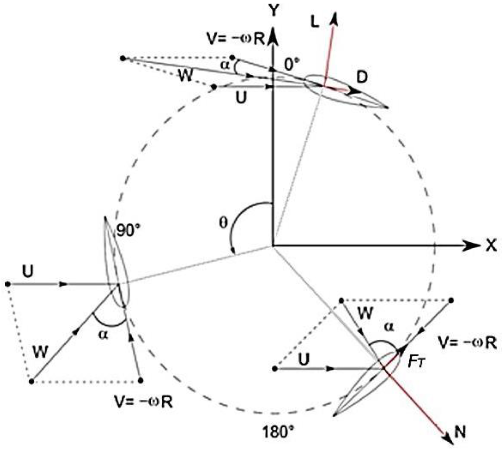
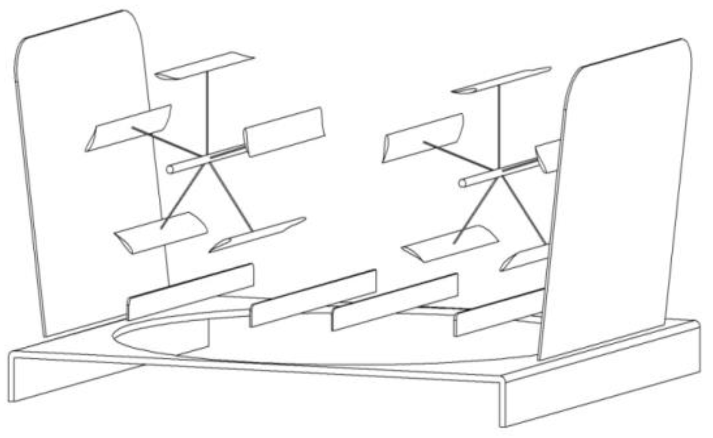
2. Working Principles of VAWT

The force and velocity distribution on a schematic VAWT is shown in Figure 1. The vector sum of the free stream wind velocity $(\overrightarrow{\mathsf{\omega }}\times \overrightarrow{R})$ and the air velocity $(\overrightarrow{U})$ is known as the relative velocity $(\overrightarrow{W})$:

$$\overrightarrow{W}=\overrightarrow{U}+(-\overrightarrow{\mathsf{\omega }}\times \overrightarrow{R})$$

(1)

Considering the orbital blade position shown in Figure 1, the maximum velocity is achieved when $\mathsf{\theta }=0°$ and the minimum velocity is at $\mathsf{\theta }=180°$.

The tip speed ratio (λ) is the ratio of the tip tangential speed of the blades (ωR) and the free-stream wind velocity; this ratio is expressed as:

$$\mathsf{\lambda }=\frac{\mathsf{\omega }R}{U}$$

(2)

According to standard airfoil theory, the lift (L) and drag (D) forces can then be used to obtain the tangential force (F_T) and the axial force N. The tangential force is the force acting along the blade’s velocity and it pulls the blade around. However, the normal force direction is toward the rotor center, pushing against the shaft bearings. The tangential force (F_T) is in charge of the generated torque and the power outputs of the VAWT.

The mechanical torque on the axis of a VAWT can be written as follows:

$$C_{t,average}=\frac{T}{\frac{1}{2}\mathsf{\rho }AR{U}^2}$$

(3)

$$C_{p,average}=\frac{P}{\frac{1}{2}\mathsf{\rho }A{U}^3}$$

(4)

where $C_{t,average}$ and $C_{\mathrm{p},average}$ are respectively the torque coefficient and the power coefficient. A is the swept turbine area and shown by the following equation:

$$A=H\times D$$

(5)

Rearranging the wind turbine power equation and considering the tip speed ratio (λ) value from Equation (3), the wind power equation can be described as:

$$P=\frac{1}{2}\mathsf{\rho }A{C}_p{U}^3=\frac{1}{2}\mathsf{\rho }A{C}_p{(\frac{\mathsf{\omega }R}{\mathsf{\lambda }})}^3$$

(6)

3. Numerical Model

In this study, the incompressible, unsteady Reynolds Average Navier-Stokes (URANS) equations are solved for the entire flow domain. The coupled pressure-based solver was selected with a second order implicit transient formulation for improved accuracy. All solution variables were solved via a second order upwind discretization scheme since most of the flow can be assumed to be not in line with the mesh [26]. The URANS vector equation is written as:

$$\frac{\partial \mathsf{\rho }U}{\partial t}+\nabla \cdot (\mathsf{\rho }UU)=-\nabla (P+\frac{2}{3}\mathsf{\mu }\nabla \cdot U)+\nabla \cdot [\mathsf{\mu }(\nabla U+{(\nabla U)}^T)]$$

(7)

Here, ρ, μ and U are the density, viscosity, and velocity respectively.

The above equation is an averaged one for the unsteady case. This unsteadiness occurs mainly due to turbulence. For incompressible flow, the continuity equation is:

$$\nabla \cdot U=0$$

(8)

The momentum equation could be simplified as:

$$\frac{\partial U}{\partial t}+\nabla \cdot (UU)=-\nabla p+\nabla \cdot ({\mathsf{\nu }}_{eff}\nabla U)$$

(9)

For ease of calculation the equation has been divided by the density. Here p is the dynamic pressure and ${\mathsf{\nu }}_{eff}$ is the effective kinematic viscosity.

Analysis System (ANSYS) Fluent computational fluid dynamics (CFD) was employed in the present study. Since the nature of VAWTs is unsteady, a transient solver was used to solve incompressible flow in a moving mesh model. Semi-Implicit Method for Pressure-Linked Equations (SIMPLE) solver was chosen for the pressure-velocity coupling. A second order scheme was used in order to solve the momentum, turbulent kinetic energy, specific dissipation rate and transient formulations.

4. Parametric Study

The unsteady nature of VAWTs has made the CFD analysis of them difficult and expensive. In order to minimize this computational cost, a precisely planned approached is required. By choosing the right parameters, such as the turbulence model, the mesh density and the time step, not only a huge amount of time can be saved but also a greater degree of accuracy can be achieved.

Almohammadi et al. [27,28], broadly analyzed the impact of mesh density in VAWT power output. In their two dimensional study, shear stress transport (SST) transitional, and $RNG-K-\mathsf{\epsilon }$ the turbulence model were tested, and it was concluded that the SST transitional was the better one. Some parametric studies were also done by Qin et al. [20]. They used $RNG-K-\mathsf{\epsilon }$ similar to one of their earlier works [29]. Although their work was in three dimensions, they carried out the parametric studies in two dimensions and they claimed to achieve mesh independency. While $RNG-K-\mathsf{\epsilon }$ is well-known to predict the vortices formation, and flow separation quite accurately, some researchers advocate the $SST-k-\mathsf{\omega }$. In addition to these two models one equation model Spalart-Allmaras was also tested in this study due to the fact that it is a single equation model and computationally less expensive [19].

The authors conducted the parametric study in two dimensions. The parametric study was carried out at a Tip Speed Ratio (λ) of 2.2.

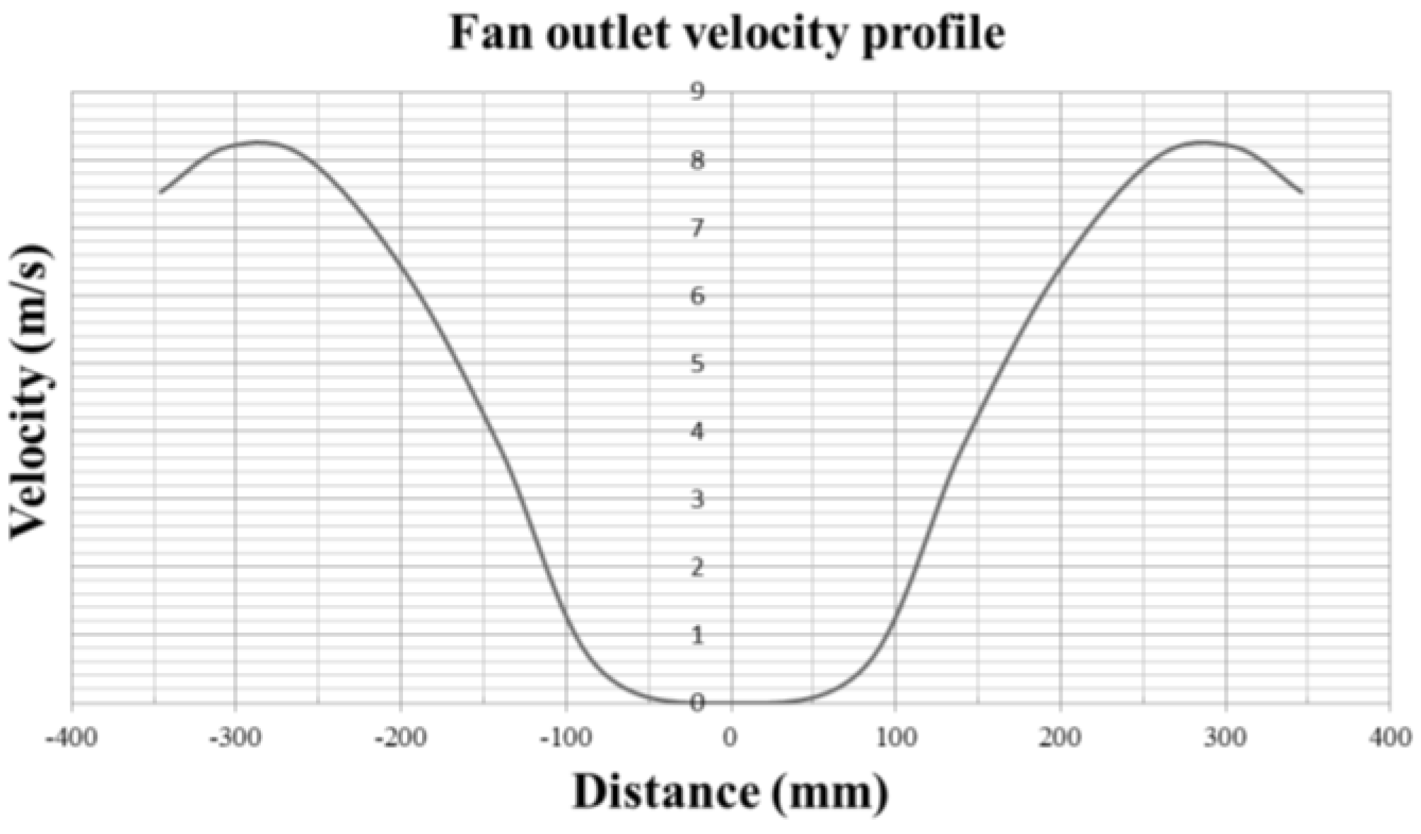
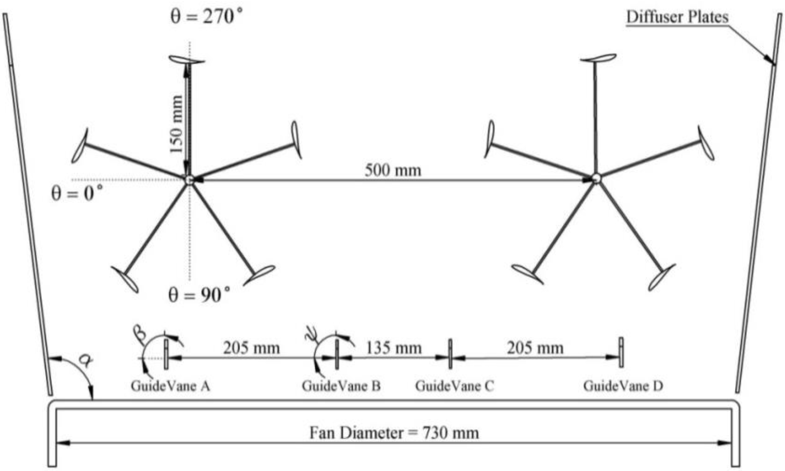
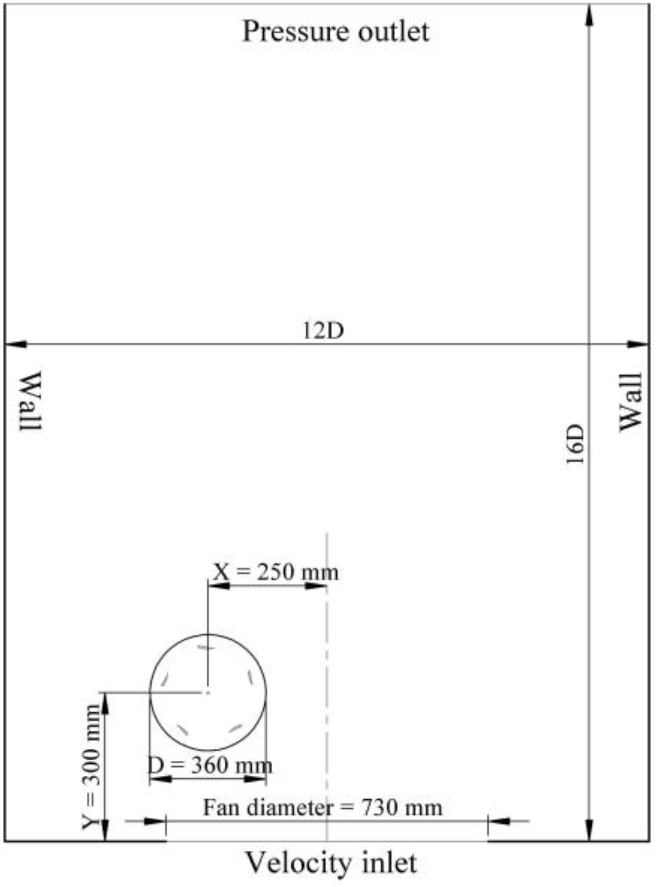
4.1. Computational Domain

In order to validate the simulation results, they were compared with the experimental data obtained in the laboratory by Fazlizan et al. [24]. Figure 2 shows the experimental apparatus used in this study.

The geometrical specifications of the computational domain used in the validation phase are shown in Figure 3. The fan diameter and the position of the VAWT can clearly be seen in this figure. All the blades are airfoil FX 63-137 with chord length of 45 mm. The rotor diameter (D_R) is 300 mm and the rotating interface diameter in 360 mm. The tip speed ratio (TSR) magnitude was assumed to be TSR = 2.2 for all cases. It means that the rotational speed of the wind turbine is assumed to be 77.5 rad/s. The fan was set at the 708 rpm which resulted in the velocity profile shown in Figure 4. This profile was then inserted to the velocity inlet boundary condition by using user defined functions (UDF).

The velocity profile of the fan at various distances is illustrated in Figure 4.

Due to the revolution of the turbine, the moving mesh approach was used for the VAWT. The rotating and fixed domains are separated by interfaces which are shown by Figure 5. The same sized mesh was selected for both sides of the interface. According to the fluent guidebook [26], the same characteristics in interface cell sizes can obtain a faster convergence. Unstructured mesh was chosen for all the domains. The generation of mesh started from the airfoils; in the grid independency test, various mesh sizes from 0.05 to 0.2 mm were applied to the airfoils. The mesh was then coarsened as it goes further to the outer domain. In order to precisely capture the flow behavior around the blade, ten boundary layers of the structural mesh were generated. In this way, the $Y_{plus}$ is also guaranteed to stay as low as 1.

To study the effect of mesh dependency, three different meshes were produced. The meshing was done following particular size functions. The refinement was only carried out on the blades. Since an enclosure is put around the blade, the refining is limited to the blade surface, and the enclosure. The stationary domain and the other portion of rotating domain remain unchanged. The mesh description is given in

Table 1. Different mesh description.

Mesh Description	M3	M2	M1
Number of cells	260,531	850,054	901,560
No. of nodes on a blade	350	700	900

. The mesh dependency study is shown in Section 4.3.

4.2. Turbulence Testing

In this study, $RNG-K-\mathsf{\epsilon }$, Spalart-Allmaras (S-A) and $SST-k-\mathsf{\omega }$ turbulence models were investigated. Except for S-A, the other two turbulence models use the turbulence kinetic energy k and the dissipation rate. For, k the value was decided using the following equation:

$$k=\frac{3}{2}\times {(UI)}^2$$

(10)

Here, U and I refer to average velocity which is 5.28 m/s (inflow) and turbulence intensity respectively. The turbulence intensity was assumed to be 5%. The value of turbulence kinetic energy is 0.1045 (m²/s²). The value of ω is obtained using the following equation:

$$\mathsf{\omega }=k^{\frac{1}{2}}/L{C}_{\mathsf{\mu }}^{\frac{1}{4}}$$

(11)

Here, L is the turbulent length scale and $C_{\mathsf{\mu }}$ is a non-dimensional constant. The turbulent length scale is assumed to be 0.01 m. The turbulence intensity represents the incoming vortices, and the turbulent length scale depicts the smallest possible diameter of the vortices.

Yahkot et al. [30] used renormalization to derive the $RNG-K-\mathsf{\epsilon }$ model from the typical $K-\mathsf{\epsilon }$ model. The main intention was to accurately model the Reynolds stress, and predict the production of dissipation terms. The number of equations increased, which leads to higher computational time. The value of $\mathsf{\epsilon }$ is derived using the following equation:

$$\mathit{∊}=C_{\mathsf{\mu }}^{\frac{1}{4}}{k}^{\frac{3}{2}}/L$$

(12)

The Spalart-Allmaras model is a one equation model which was designed with the objective of numerical efficiency. As it is a one equation model, it is much faster than the $RNG-k-\mathsf{\epsilon }$ model. This model is effective for wall-bounded and adverse pressure gradient flows in the boundary layer. However this model is known to perform poorly in laminar to turbulent transition.

The $SST-k-\mathsf{\omega }$ model is an improved version of the standard $k-\mathsf{\omega }$ model. It uses the original Wilcox $k-\mathsf{\omega }$ formulation near walls. Again it switches to $k-\mathsf{\epsilon }$ behavior while resolving the free stream. The adjustment of eddy viscosity formulation enables this model to accurately deal with the transport effects of the turbulent shear stress. As a result, it avoids the common problem associated with the standard $k-\mathsf{\omega }$ model.

Achieving convergence in the unsteady case of VAWT is time consuming especially for the convergence criteria of 10⁻⁵ which is used in this study. In order to achieve convergence in a reasonable time, under relaxation is put to use. An under-relaxation factor of 0.3 for the pressure equation, 0.7 for turbulent kinetic energy k, and 0.8 for the velocity equation are used.

The deviation between the torque coefficient obtained from the fourth and fifth revolution is less than 5%. Therefore, it was assumed that the steady periodic output was achieved after 4–5 revolutions. It can be seen from

Table 2. Numerical and experimental results.

Description	Power Coefficient	Computational Time for 1 s of Computational Case
RNG k-epsilon	0.0820	45.2 h
SST k-omega	0.1003	48.6 h
S-A	0.114	31.4 h
Experimental	0.0918	-

RNG, re-normalisation group; SST, shear stress transport; S-A, Spalart-Allmaras.

that the result obtained from the $SST-k-\mathsf{\omega }$ model is the closest one to the experimental value. In the simulation, the influence of the rotating and support arm was ignored. If these entities had been included the outcome would have been different. The value of the Power coefficient (C_P) would have been reduced.

Therefore, $SST-k-\mathsf{\omega }$ was selected as the turbulence model in this study. Since the system is characterized by a low Reynolds number, the $k-\mathsf{\epsilon }$ and the Spallart-Allmaras model cannot capture and predict the flow development, especially in laminar separation bubbles. Thus, the $SST-k-\mathsf{\omega }$ model can be utilized as a low Reynolds turbulence model without any extra damping functions. Furthermore, this model is able to provide a very good prediction of the turbulence in adverse pressure gradients and separating flow. Furthermore, the shear stress transport (SST) formulation is formed by combining the $k-\mathsf{\omega }$ and $k-\mathsf{\epsilon }$ models. This structure assists the SST method to switch to the $k-\mathsf{\epsilon }$ model in order to avoid the $k-\mathsf{\omega }$ problem in the inlet free-stream turbulence properties and to use the $k-\mathsf{\omega }$ formulation in the inner parts of the boundary layer.

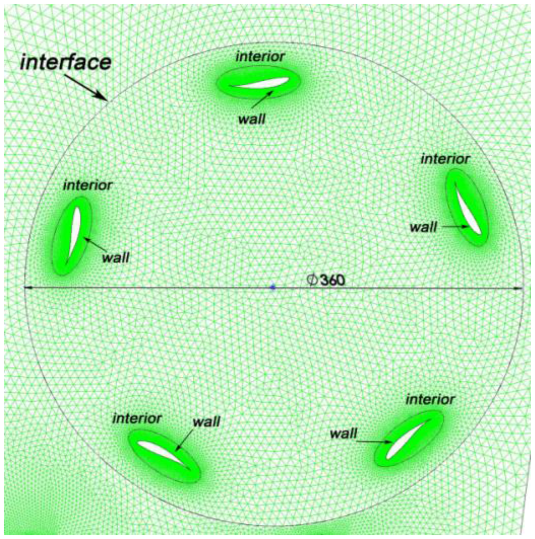
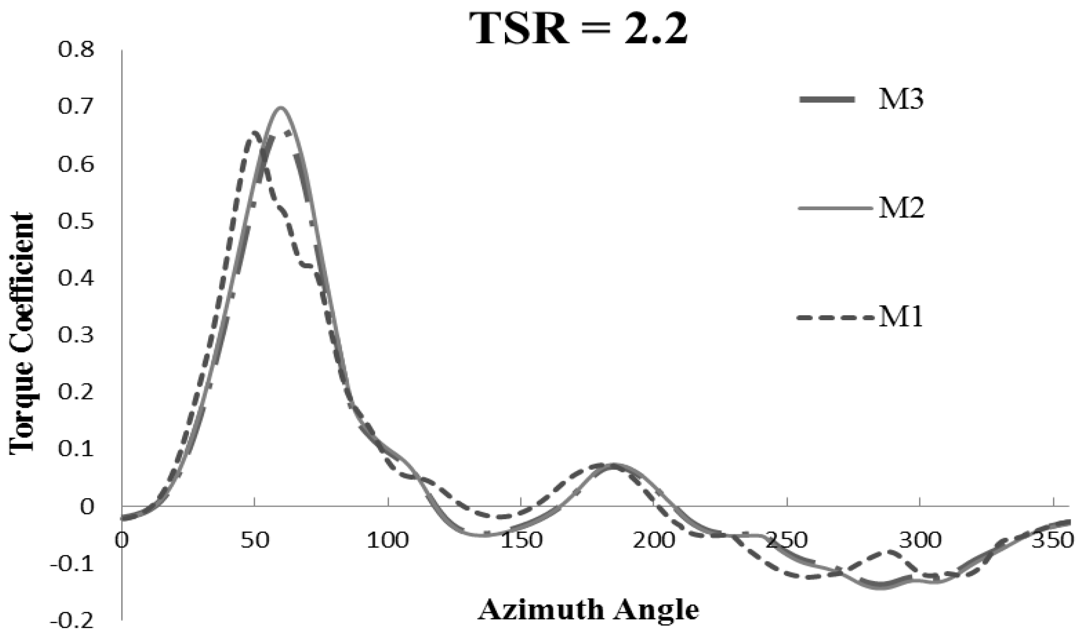
4.3. Mesh Dependency Study

Table 1 gives the specifications of meshes used in this study. The authors used the power coefficient of VAWT for the mesh independency check. In the case of the wind turbine the quantity considered to be the most important one is performance. Roache et al. [26] described the method of using Richardson extrapolation for finding the required mesh resolution and convergence. Almohammadi et al. [28] also used the method. The mesh resolution required for an accurate result is identified as:

$$C{p}_{exact}=\overline{C}{p}_1+\frac{C{p}_1-C{p}_2}{r^P-1}+\text{Higher order truncation}$$

(13)

Here the subscripts refer to different mesh resolution levels. The quantity p denotes the order of accuracy and the order of accuracy was assumed to be 2. As for catching vortices and resolving dynamic stall, high resolution meshing was provided near the blade, there was no need to refine other parts of the computational domain. The process of refining is briefly discussed in Section 4.1. The apparent convergence study is defined by the following equation:

$$R^{*}=\frac{C{p}_2-C{p}_1}{C{p}_3-C{p}_2}$$

(14)

• If,
• R* >1 Monotonic divergence
• 1 > R* > 0 Monotonic convergence
• 0 > R*> −1 Oscillatory convergence
• R* < −1 Oscillatory divergence

The mesh convergence was found to be (−0.641). So it is an oscillatory convergence case. It can successfully be concluded that the mesh dependency is achieved and depicted by Figure 6.

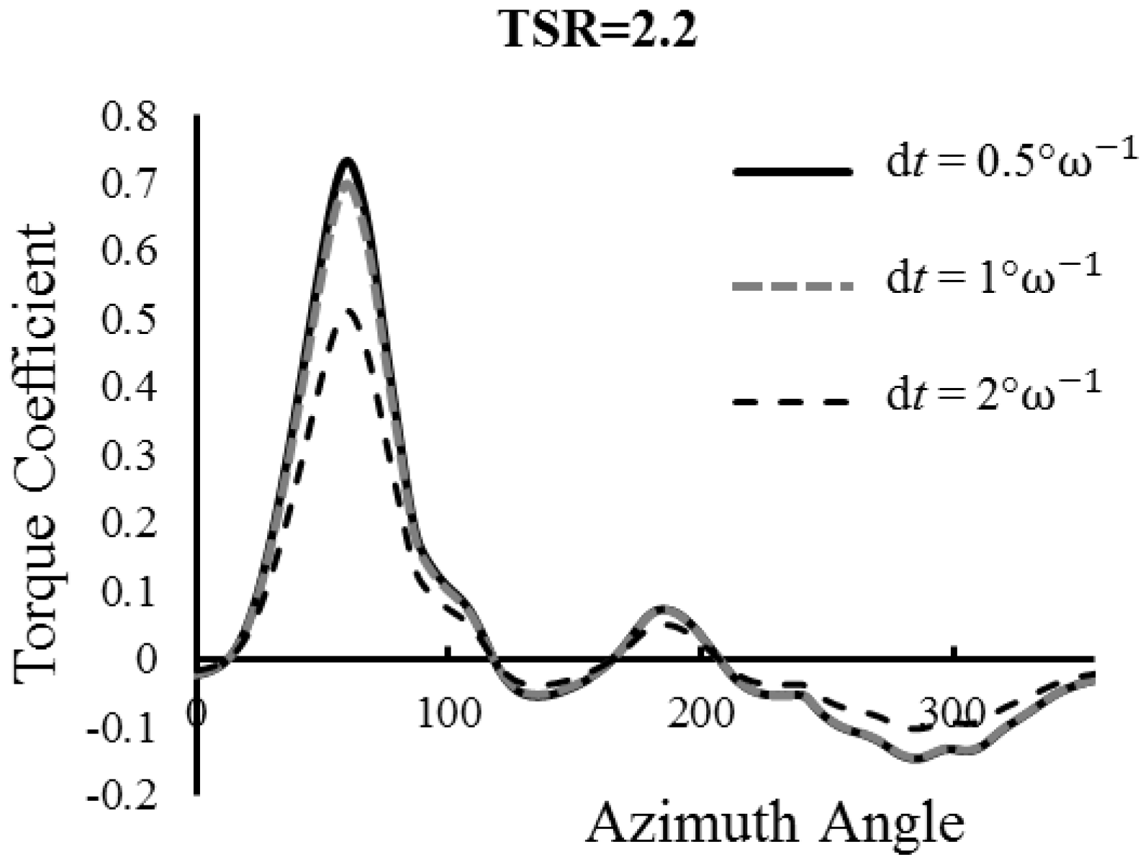
4.4. Dependency of Time Increment

The accuracy and convergence of a CFD study is highly dependent on choosing the right time step [20]. Four different time steps were considered, based on the VAWT rotational speed, to achieve a reliable result. The largest dt was equal to 3°ω⁻¹; equivalent to three degree rotation and the smallest one was 0.5°ω⁻¹; equivalent to half a degree rotation when the tip speed ratio was 2.2.

As Figure 7 illustrates, a trivial difference between torque coefficient of dt = 1°ω⁻¹ and 0.5°ω⁻¹ existed. Therefore, a time step of 1°ω⁻¹ (0.00025 s) was chosen for successive numerical simulations in order to save computational time and cost.

4.5. Final Parameters

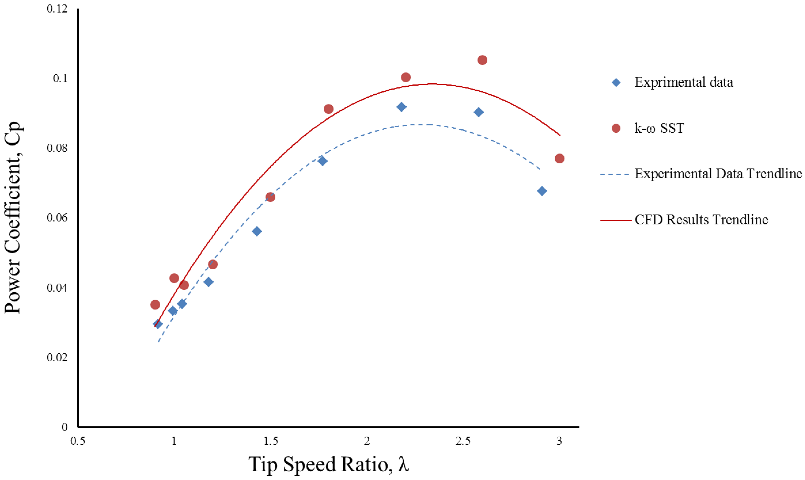
From the discussion of the turbulence models it is evident that S-A is not compatible with the present objectives. The performance of $RNG-k-\mathsf{\epsilon }$ and $SST-k-\mathsf{\omega }$ is almost similar. However, $SST-k-\mathsf{\omega }$ is believed to capture the wake vortices better than $RNG-k-\mathsf{\epsilon }$. Again, the result obtained from $SST-k-\mathsf{\omega }$ is the closest to the experimental value. This is why the turbulence model $SST-k-\mathsf{\omega }$ was chosen. As seen from the mesh dependency analysis, the result obtained from the finest mesh M-3 does not differ much from the medium fine mesh M-2. This is why the M-2 mesh was chosen. Finally, the chosen time step was 1°ω⁻¹ equal to 0.00025 s.

4.6. CFD Validation

The researchers in the Mechanical Department of the University of Malaya carried out several experiments, and an analytical study [4,6,22,23,24,31,32] on VAWT performance. The simulation result of this study was verified using the experimental data obtain by Fazlizan et al. [24]. The specification of the experimental setup and the computational domain are described in Section 4.1. The simulations were done for seven revolutions. The results were obtained from the last three revolutions.

Figure 8 shows the comparison of the power coefficient between CFD simulation and the experimental result for TSR in the range of 0.9 to 3.0. The simulation result is in good agreement with the experimental values [24]. The discrepancies may occur due to insufficient mesh resolution, and turbulence modeling. The turbulence model and computational domain of this study were chosen after parametric studies. These studies were conducted in TSR 2.2. According to the popular definition of Reynolds number of a wind turbine, the characteristic length should be the diameter of the rotor disc. The Reynolds number in this study was 1.58 × 10⁵. However the blades experience relative velocity with the change of TSR, and the Reynolds number varies from 1.38 × 10⁵ to 1.90 × 10⁶. In this range both laminar and turbulent flow is expected around the blade. Resolving the transition from laminar to turbulent flow is not easy. Conventionally, parameters obtained from a parametric study are valid for the specific Reynolds number, at which the study is administered. As the parametric study is carried out in TSR 2.2, it can be observed from Figure 8 that the simulation values near TSR 2.2 are comparatively closer to the experimental ones than the other TSRs. However the range of varying Reynolds number in this study is not that high. Again the deviations of the present study are in a satisfactory range in comparison to some existing papers [20,29].

5. Results and Discussion

In order to improve this design, two diffuser plates and four guide vanes as well as an extra VAWT were introduced to it which resulted to the design shown in Figure 9.

A detailed two dimensional model of the proposed design is illustrated in Figure 10. The effect of added features of the VAWT performance is discussed in the following sections.

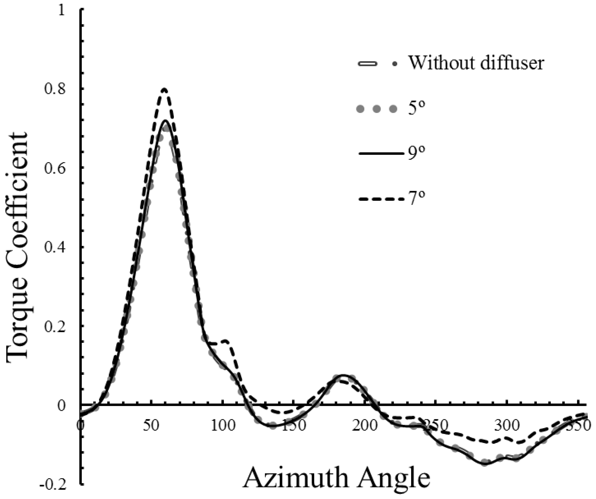
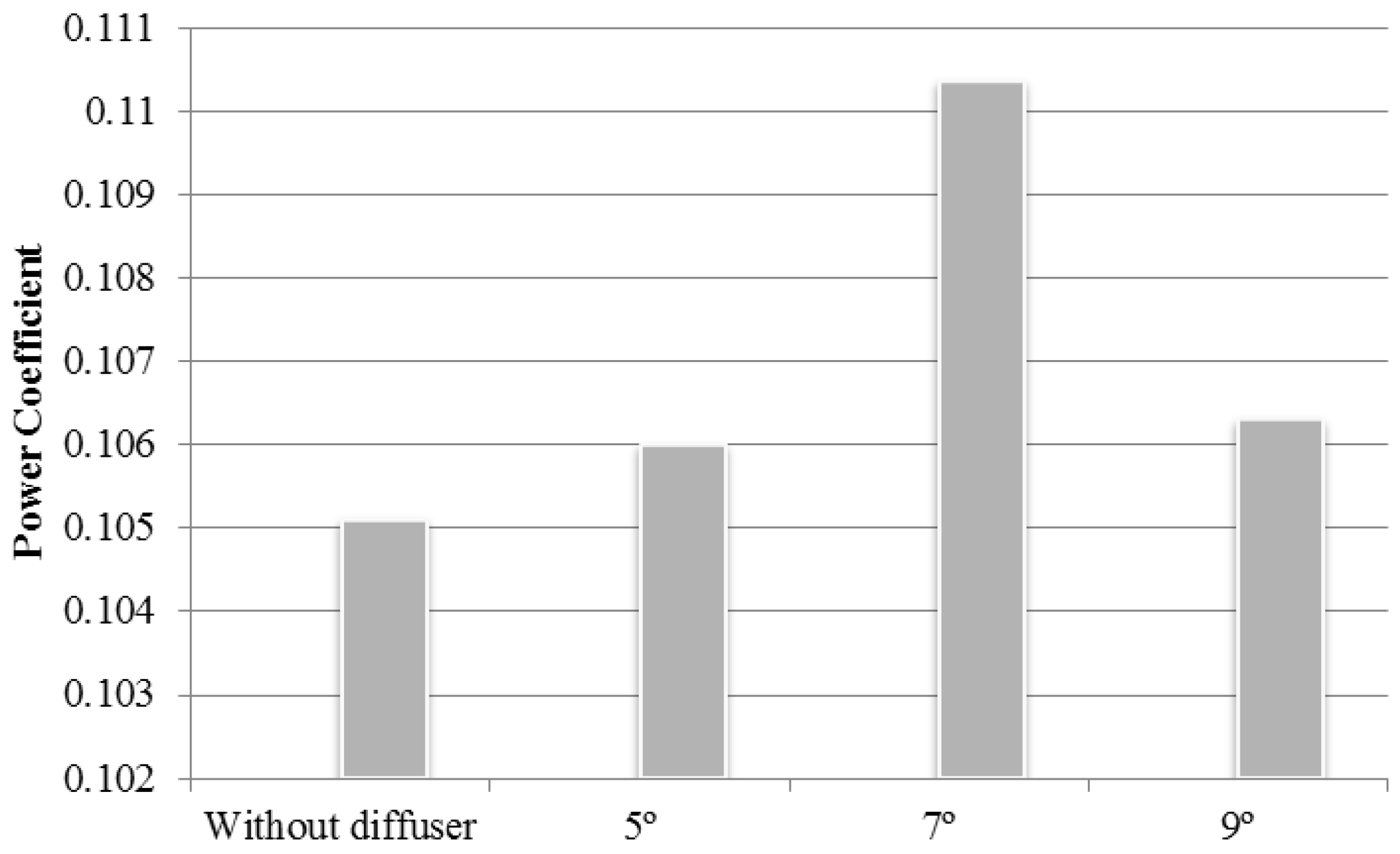
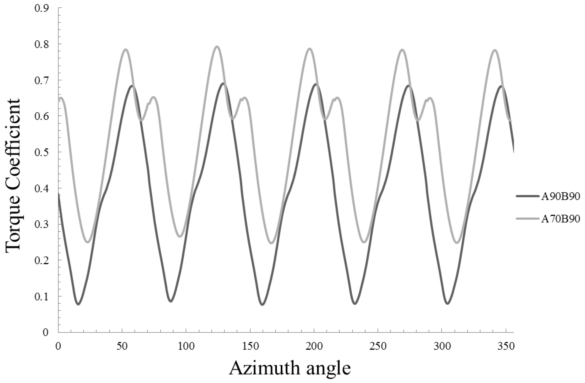
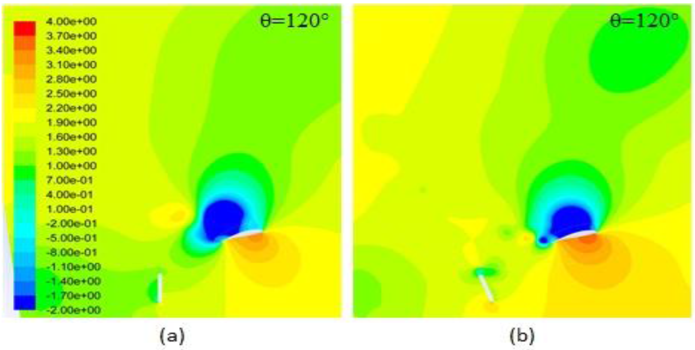
5.1. The Effect of the Diffuser Angle

As can be understood from Equation (6), the generated power is hugely correlative to the cubed wind speed. Therefore, by even a minor increment in the wind velocity, a considerable increase in power output can be obtained. Enhancement of the wind velocity around a wind turbine by using the fluid dynamic nature, especially by concentrating the wind energy locally, has always been considered an effective way to boost the wind turbine’s output power.

Wind-concentrating devices known as diffusers have been widely employed in wind turbines in order to enhance the power generation. According to the basic laws of conservation of mass and energy—called Bernoulli’s law—the mass flow is proportional to the area ratio $(A_{exit}/A_{\mathit{in}\mathrm{flow}})$. Therefore, more mass flow can be increased if the exit area of the fluid is larger than its inflow area. Unfortunately, nature is not that generous. To be more precise, opening angles less than 10° have to be used to avoid what is called flow separation [33]. Therefore in this study, 5°, 7°, and 9° were selected for the diffuser plates’ angle (α). The engineering task then is to find a reasonable area ratio. Serious work started in 1956 by Liley and Rainbird [34] and efforts up to 2007 were summarized by van Bussel [35].

At the first step, two diffuser plates with three different angles were introduced while guide vanes A and B were kept at 90°. The TSR in all cases, the same as the parametric study section, was assumed to be 2.2. The comparison of the torque coefficients obtained from a single blade in each arrangement is shown in Figure 11. As is clear, the diffuser with 7° has the higher peak as well as a more positive torque area. Figure 12 illustrates the power output for the four different designs. While the diffuser with 5° and 9° degree shows almost the same amount, the 7° diffuser improves the power by almost 5% compared to the design without diffusers. It is thus concluded that the optimum angle for the diffuser plates is 7°. This result is in good agreement with the experimental data achieved by Chong et al. [22] and previous research done by Abe et al. [36].

This improvement is justified by considering the fact that the diffuser-plates are causing a flow augmentation effect, which leads to a discharged airflow increment based on Bernoulli’s principle. Ultimately, this increased volumetric flow rate interacts with the VAWT blades, resulting in a higher energy output.

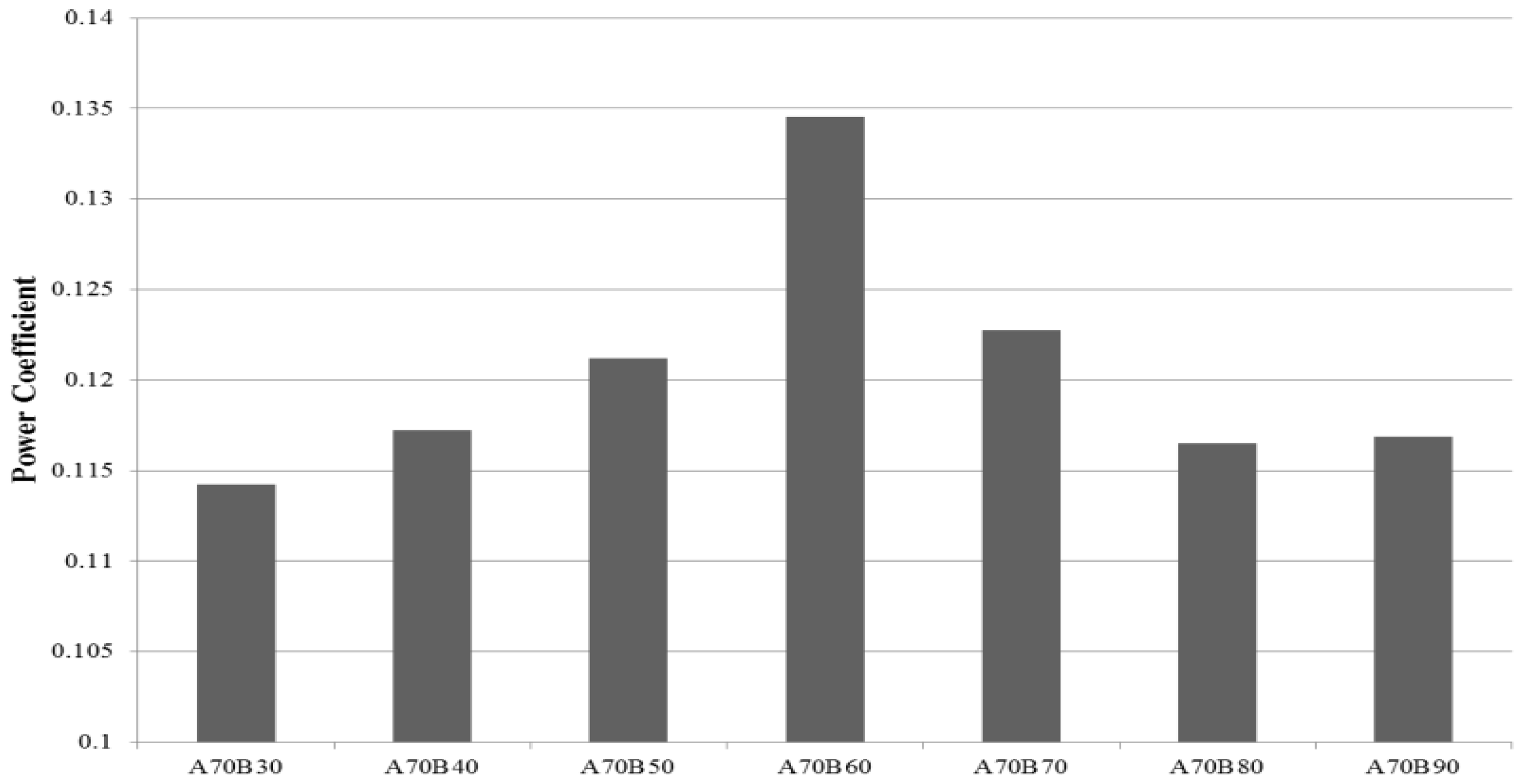
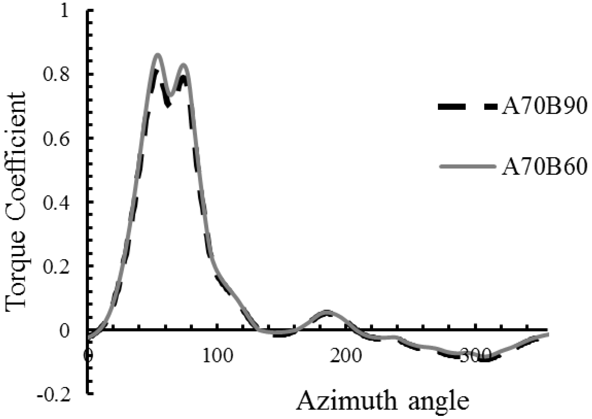
5.2. The Effect of Guide Vanes

Considering the optimum angle of the diffuser plates to be 7°, the next step is to change the angles of the guide vanes. This step was done in two stages by rotating a single guide vane at each stage.

5.2.1. Guide Vane A

The effects of eleven different angles in the range of 30° to 130° with intervals of 10 are studied in this stage. The principle behind the guide vanes are the same as the diffuser. They are capable of creating low pressure zones and consequently increasing the air flow speed. As is clear from Figure 13, the guide vane with an angle of 70° provides the highest output power among all the other arrangements. One of the reasons that the 30° and 130° guide vanes provide the lowest power coefficient is that they mostly acted as a blockage for inlet wind by creating a large wake behind themselves.

The results and other specifications of the tests are tabulated in

Table 3. The results and other specifications of the various cases.

	Cm	T	TSR	Cp	P	Deviation from Baseline Design (%)
A30B90	0.032	0.024	2.2	0.071	1.86	−31.6176
A40B90	0.045	0.033	2.2	0.099	2.59	−4.77941
A50B90	0.045	0.033	2.2	0.098	2.57	−5.51471
A60B90	0.049	0.036	2.2	0.108	2.82	3.676471
A70B90	0.053	0.039	2.2	0.116	3.03	11.39706
A80B90	0.046	0.033	2.2	0.101	2.63	−3.30882
A90B90	0.047	0.035	2.2	0.105	2.72	0
A100B90	0.038	0.028	2.2	0.083	2.18	−19.8529
A110B90	0.042	0.031	2.2	0.093	2.42	−11.0294
A120B90	0.045	0.033	2.2	0.099	2.57	−5.51471
A130B90	0.036	0.027	2.2	0.08	2.09	−23.1618

C_m, coefficient of momentum; T, torque; TSR, tip speed ratio; C_p, coefficient of power; P, generated power.

. The numbers after the letters A and B indicate the guide vane angles of β and ψ (see Figure 10). The torque (T) and power coefficient (C_p) were calculated using Equations (4) and (5), respectively. This table also indicates that β = 70° results in the highest power output. The relative deviations of the output power compared to the baseline design, when both β and ψ are equal to 90°, are also tabulated in Table 3.

Figure 14 compares the variation in the torque coefficient of the two different arrangements for a complete revolution. As clear, although before the azimuth angle of 90° the figures are almost identical, the 70° guide vane provides a higher torque coefficient afterwards^, which leads to a higher average power coefficient. This increase can be more clearly observed in Figure 15, where the total torque coefficient of all five blades is shown. As is apparent utilization of the 70° guide vane provided a considerable enhancement in produced torque. Even though it is out of this study scope, it is noteworthy that this modification in design decreased the fluctuation rate in the torque diagram which can result in less fatigue in the VAWT.

According to Figure 15, the most significant difference in torque coefficient for the two cases of β = 90° and 70° occurs when 90° < θ < 180°. Therefore, the contour of the pressure coefficient at θ = 120° was plotted in Figure 16 to investigate the possible reason for this increment. It can be observed in this figure that when the 70° guide vane is used the distribution of the low pressure zone on the top of the blade is significantly improved. This phenomenon caused more pressure difference between the low and top of the blade leading to a higher torque.

5.2.2. Guide Vane B

The next stage proceeded by fixing the guide vane at β = 70°. Seven different arrangements in the range of ψ = 30° to 90° with 10 intervals were considered for guide vane B. Due to the position of this guide vane, angles greater than 90° were ignored. As is obvious in Figure 17, the greatest power coefficient belongs to the arrangement with ψ = 60° when it is equal to 0.134.

The results and other specifications of the tests are shown in

Table 4. The results and other specifications of the various cases.

	Cm	T	TSR	Cp	P	Deviation from Baseline Design (%)
A70B30	0.051	0.038	2.2	0.114	2.96	8.823529
A70B40	0.053	0.039	2.2	0.117	3.04	11.76471
A70B50	0.055	0.04	2.2	0.121	3.15	15.80882
A70B60	0.061	0.045	2.2	0.134	3.49	28.30882
A70B70	0.055	0.041	2.2	0.122	3.19	17.27941
A70B80	0.052	0.039	2.2	0.1165	3.02	11.02941
A70B90	0.053	0.0392	2.2	0.1168	3.03	11.39706

C_m, coefficient of momentum; T, torque; TSR, tip speed ratio; C_p, coefficient of power; P, generated power.

. From this table it is indicated that ψ = 60° results in the highest power output with 3.49 W. The first column from the right shows the relative deviations of the output power from the baseline design, when both β and ψ are equal to 90°, are also tabulated in Table 3.

The torque coefficient variation in two different arrangements for a complete revolution is compared in Figure 18. As it is clear, from θ = 0° to θ = 160°, both diagrams are relatively congruent; however, after this point the torque coefficient related to ψ = 60° is considerably higher until the end of the cycle, leading to a 15% higher average torque coefficient.

6. Economic Feasibility

A techno-economic analysis has been carried out on the novel exhaust air energy recovery wind turbine generator installed on a cooling tower commonly used in Malaysia. For the cooling tower with a 7.5 kW rated fan motor, 13.3% of the discharged energy is expected to be recovered. For a year of operation of the cooling tower with this system, approximately 7.3 MWh is estimated to be recovered. Economic analysis shows that capital, components replacement, as well as operation and maintenance costs of the system are covered in the lifetime of the system. For this project, the net present (NPV) is 25,347 Malaysian Ringgit (RM) for the 20-year lifetime.

7. Conclusions

A 2D CFD study was carried out on a novel wind turbine design. The effects of different diffuser plate angles and guide vane angles were investigated. It was derived from the results that by introducing diffusers and then guide vanes, the overall power output of the wind turbine was improved by approximately 5% and 34%, respectively, compared to using a VAWT alone. In the case of the diffusers, the optimum angle was found to be 7°, while for guide vanes A and B, it was 70° and 60°, respectively. These results are in good agreement with experimental results obtained in the laboratory. Overall, it can be concluded that exhaust air recovery turbines offer a promising opportunity in green technology.

References

1. Manwell, J.F.; McGowan, J.G.; Rogers, A.L. Wind Energy Explained: Theory, Design and Application; John Wiley & Sons: Hoboken, NJ, USA, 2010. [Google Scholar]
2. Energy Commission of Malaysia. Malaysia Energy Statistics Handbook 2014; Suruhanjaya Tenaga: Putrajaya, Malaysia. Available online: http://www.meih.st.gov.my (accessed on 24 May 2015).
3. Sung, C.T.B. Possibility of electricity from wind energy in Malaysia: Some rough calculations. Available online: http://www.christopherteh.com/blog/2010/11/wind-energy/ (accessed on 24 May 2015).
4. Chong, W.T.; Fazlizan, A.; Poh, S.C.; Pan, K.C.; Hew, W.P.; Hsiao, F.B. The design, simulation and testing of an urban vertical axis wind turbine with the omni-direction-guide-vane. Appl. Energy 2013, 112, 601–609. [Google Scholar] [CrossRef]
5. Ohya, Y.; Karasudani, T. A shrouded wind turbine generating high output power with wind-lens technology. Energies 2010, 3, 634–649. [Google Scholar] [CrossRef]
6. Chong, W.T.; Pan, K.C.; Poh, S.C.; Fazlizan, A.; Oon, C.S.; Badarudin, A.; Nik-Ghazali, N. Performance investigation of a power augmented vertical axis wind turbine for urban high-rise application. Renew. Energy 2013, 51, 388–397. [Google Scholar] [CrossRef]
7. Foreman, K.; Gilbert, B. Technical development of the Diffuser Augmented Wind Turbine/DAWT/concept. Wind Eng. 1979, 3, 153–166. [Google Scholar]
8. Foreman, K.; Gilbert, B.; Oman, R. Diffuser augmentation of wind turbines. Solar Energy 1978, 20, 305–311. [Google Scholar] [CrossRef]
9. Foreman, K. Preliminary Design and Economic Investigations of Diffuser-Augmented Wind Turbines (DAWT); Grumman Aerospace Corp.: Bethpage, NY, USA, 1981. [Google Scholar]
10. Moeller, M.; Visser, K. Experimental and numerical studies of a high solidity, low tip speed ratio DAWT. In Proceedings of the 48th AIAA Aerospace Sciences Meeting and Exhibit, Orlando, FL, USA, 4–7 January 2010.
11. Tong, C.W.; Chew, P.S.; Abdullah, A.F.; Sean, O.C.; Ching, T.C. Exhaust air and wind energy recovery system for clean energy generation. In Proceedings of the International Conference on Environment and Industrial Innovation, Kuala Lumpur, Malaysia, 4–5 June 2011; IACSIT Press: Kuala Lumpur, Malaysia, 2011. [Google Scholar]
12. Shahizare, B.; Ghazali, N.N.B.N.; Chong, W.T.; Tabatabaeikia, S.; Izadyar, N. Investigation of the optimal omni-direction-guide-vane design for vertical axis wind turbines based on unsteady flow CFD simulation. Energies 2016, 9, 146. [Google Scholar] [CrossRef]
13. Shahizare, B.; Nik-Ghazali, N.; Chong, W.; Tabatabaeikia, S.; Izadyar, N.; Esmaeilzadeh, A. Novel investigation of the different Omni-direction-guide-vane angles effects on the urban vertical axis wind turbine output power via three-dimensional numerical simulation. Energy Conv. Manag. 2016, 117, 206–217. [Google Scholar] [CrossRef]
14. Mertens, S.; van Kuik, G.; van Bussel, G. Performance of an H-Darrieus in the skewed flow on a roof. J. Sol. Energy Eng. 2003, 125, 433–440. [Google Scholar] [CrossRef]
15. Simms, D.A.; Schreck, S.; Hand, M.; Fingersh, L. NREL Unsteady Aerodynamics Experiment in the NASA-Ames Wind Tunnel: A Comparison of Predictions to Measurements; National Renewable Energy Laboratory: Golden, CO, USA, 2001. [Google Scholar]
16. McTavish, S.; Feszty, D.; Sankar, T. Steady and rotating computational fluid dynamics simulations of a novel vertical axis wind turbine for small-scale power generation. Renew. Energy 2012, 41, 171–179. [Google Scholar] [CrossRef]
17. McLaren, K.; Tullis, S.; Ziada, S. Computational fluid dynamics simulation of the aerodynamics of a high solidity, small-scale vertical axis wind turbine. Wind Energy 2012, 15, 349–361. [Google Scholar] [CrossRef]
18. Edwards, J.M.; Danao, L.A.; Howell, R.J. Novel experimental power curve determination and computational methods for the performance analysis of vertical axis wind turbines. J. Sol. Energy Eng. 2012, 134. [Google Scholar] [CrossRef]
19. Chowdhury, A.M.; Akimoto, H.; Hara, Y. Comparative CFD analysis of Vertical Axis Wind Turbine in upright and tilted configuration. Renew. Energy 2016, 85, 327–337. [Google Scholar] [CrossRef]
20. Qin, N.; Howell, R.; Durrani, N.; Hamada, K.; Smith, T. Unsteady flow simulation and dynamic stall behaviour of vertical axis wind turbine blades. Wind Eng. 2011, 35, 511–528. [Google Scholar] [CrossRef]
21. Castelli, M.R.; Englaro, A.; Benini, E. The Darrieus wind turbine: Proposal for a new performance prediction model based on CFD. Energy 2011, 36, 4919–4934. [Google Scholar] [CrossRef]
22. Chong, W.T.; Hew, W.P.; Yip, S.Y.; Fazlizan, A.; Poh, S.C.; Tan, C.J.; Ong, H.C. The experimental study on the wind turbine’s guide-vanes and diffuser of an exhaust air energy recovery system integrated with the cooling tower. Energy Convers. Manag. 2014, 87, 145–155. [Google Scholar] [CrossRef]
23. Chong, W.T.; Fazlizan, A.; Poh, S.C.; Pan, K.C.; Ping, H.W. Early development of an innovative building integrated wind, solar and rain water harvester for urban high rise application. Energy Build. 2012, 47, 201–207. [Google Scholar] [CrossRef]
24. Fazlizan, A.; Chong, W.; Yip, S.; Hew, W.; Poh, S. Design and experimental analysis of an exhaust air energy recovery wind turbine generator. Energies 2015, 8, 6566–6584. [Google Scholar] [CrossRef]
25. Paraschivoiu, I. Wind Turbine Design: With Emphasis on Darrieus Concept; Presses Inter Polytechnique: Montréal, QC, Canada, 2002. [Google Scholar]
26. Fluent, A. 14.5 User’s Guide; Fluent Inc.: New York, NY, USA, 2012. [Google Scholar]
27. Almohammadi, K.; Ingham, D.; Ma, L.; Pourkashanian, M. CFD sensitivity analysis of a straight-blade vertical axis wind turbine. Wind Eng. 2012, 36, 571–588. [Google Scholar] [CrossRef]
28. Almohammadi, K.M.; Ingham, D.B.; Ma, L.; Pourkashan, M. Computational fluid dynamics (CFD) mesh independency techniques for a straight blade vertical axis wind turbine. Energy 2013, 58, 483–493. [Google Scholar] [CrossRef]
29. Howell, R.; Qin, N.; Edwards, J.; Durrani, N. Wind tunnel and numerical study of a small vertical axis wind turbine. Renew. Energy 2010, 35, 412–422. [Google Scholar] [CrossRef]
30. Yakhot, V.; Orszag, S.; Thangam, S.; Gatski, T.; Speziale, C. Development of turbulence models for shear flows by a double expansion technique. Phys. Fluids A Fluid Dyn. (1989–1993) 1992, 4, 1510–1520. [Google Scholar] [CrossRef]
31. Chong, W.T.; Naghavi, M.S.; Poh, S.C.; Mahlia, T.M.I.; Pan, K.C. Techno-economic analysis of a wind-solar hybrid renewable energy system with rainwater collection feature for urban high-rise application. Appl. Energy 2011, 88, 4067–4077. [Google Scholar] [CrossRef]
32. Lim, Y.C.; Chong, W.T.; Hsiao, F.B. Performance Investigation and Optimization of a Vertical Axis Wind Turbine with the Omni-Direction-Guide-Vane. Procedia Eng. 2013, 67, 59–69. [Google Scholar] [CrossRef]
33. Schaffarczyk, A. Introduction to Wind Turbine Aerodynamics; Springer: Berlin, Germany, 2014. [Google Scholar]
34. Lilley, G.; Rainbird, W. A Preliminary Report on the Design and Performance of Ducted Windmills; College of Aeronautics Cranfield: Cranfield, UK, 1956. [Google Scholar]
35. Van Bussel, G.J. The science of making more torque from wind: Diffuser experiments and theory revisited. In Journal of Physics: Conference Series; IOP Publishing: Bristol, UK, 2007. [Google Scholar]
36. Abe, K.; Nishida, M.; Sakurai, A.; Ohya, Y.; Kihara, H.; Wada, E.; Sato, K. Experimental and numerical investigations of flow fields behind a small wind turbine with a flanged diffuser. J. Wind Eng. Ind. Aerodyn. 2005, 93, 951–970. [Google Scholar] [CrossRef]
Figure 1. Force and velocity distribution on a vertical axis wind turbines (VAWT) [25]
Energies 09 00346 g001
Figure 2. Experimental apparatus.
Energies 09 00346 g002
Figure 3. Computational domain.
Energies 09 00346 g003
Figure 4. Exhaust fan velocity profile.
Energies 09 00346 g004
Figure 5. Mesh of rotating area.
Energies 09 00346 g005
Figure 6. Variation of torque coefficient by azimuth angle for different mesh densities at tip speed ratio (TSR) = 2.2.
Energies 09 00346 g006
Figure 7. Time dependency study.
Energies 09 00346 g007
Figure 8. Power coefficients obtained by computational fluid dynamics (CFD) simulation and experimental result.
Energies 09 00346 g008
Figure 9. Iso-metric view of the augmented exhaust air energy recovery turbine.
Energies 09 00346 g009
Figure 10. Two-dimensional (2D) model of the exhaust air energy recovery turbine.
Energies 09 00346 g010
Figure 11. Effect of angle of diffusers on torque coefficient.
Energies 09 00346 g011
Figure 12. Power coefficient of different diffuser plate arrangements.
Energies 09 00346 g012
Figure 13. Effect of guide vane “A” angle on power coefficient.
Energies 09 00346 g013
Figure 14. Torque coefficient of a single blade.
Energies 09 00346 g014
Figure 15. Total torque coefficient of five blades.
Energies 09 00346 g015
Figure 16. Pressure coefficient contour. (a) β = 90° and (b) β = 70°.
Energies 09 00346 g016
Figure 17. Effect of guide vane B angle on power coefficient.
Energies 09 00346 g017
Figure 18. Torque coefficient of a single blade.
Energies 09 00346 g018