High Spatial Resolution Simulation of Annual Wind Energy Yield Using Near-Surface Wind Speed Time Series

Abstract

In this paper a methodology is presented that can be used to model the annual wind energy yield (AEY_mod) on a high spatial resolution (50 m × 50 m) grid based on long-term (1979–2010) near-surface wind speed (U_S) time series measured at 58 stations of the German Weather Service (DWD). The study area for which AEY_mod is quantified is the German federal state of Baden-Wuerttemberg. Comparability of the wind speed time series was ensured by gap filling, homogenization and detrending. The U_S values were extrapolated to the height 100 m (U_100m,emp) above ground level (AGL) by the Hellman power law. All U_100m,emp time series were then converted to empirical cumulative distribution functions (CDF_emp). 67 theoretical cumulative distribution functions (CDF) were fitted to all CDF_emp and their goodness of fit (GoF) was evaluated. It turned out that the five-parameter Wakeby distribution (WK5) is universally applicable in the study area. Prior to the least squares boosting (LSBoost)-based modeling of WK5 parameters, 92 predictor variables were obtained from: (i) a digital terrain model (DTM), (ii) the European Centre for Medium-Range Weather Forecasts re-analysis (ERA)-Interim reanalysis wind speed data available at the 850 hPa pressure level (U_850hPa), and (iii) the Coordination of Information on the Environment (CORINE) Land Cover (CLC) data. On the basis of predictor importance (PI) and the evaluation of model accuracy, the combination of predictor variables that provides the best discrimination between U_100m,emp and the modeled wind speed at 100 m AGL (U_100m,mod), was identified. Results from relative PI-evaluation demonstrate that the most important predictor variables are relative elevation (Φ) and topographic exposure (τ) in the main wind direction. Since all WK5 parameters are available, any manufacturer power curve can easily be applied to quantify AEY_mod.

1. Introduction

The world’s energy supply is facing multiple challenges. The depletion of conventional fuels is unavoidable [1,2], greenhouse gas emissions from the burning of fossil fuels most significantly contributes to global warming [3,4] and the emissions of air pollutants affect human health [3,5]. Although nuclear energy production enables the reduction of carbon dioxide (CO₂) emissions [6], nuclear power plants bear great short- and long-term risk of accidents [7]. In order to reduce and avoid negative impacts of the current use of energy resources on the environment and human health, alternative forms of energy utilization must be found.

Renewable energies provide a clean, environmentally friendly and health-compatible alternative to fossil energies and nuclear energy [2,5]. One major renewable energy resource is the kinetic energy contained in the atmosphere, commonly known as wind energy. The potential for wind energy utilization to play a key role in the future global energy mix is enormous. Wind energy could supply more than 40 times [8] the annual global electricity consumption. Consequently, the wind power generation capacity of the world is growing constantly with an average annual rate of about 30% over the last decade [2]. In the European Union, directive 2009/28/EC [9] aims to cover 20% of the primary energy demand by renewable energies in 2020, including wind energy. The leading wind power producer in Europe is Germany. Germany aims to supply at least 30% of the energy consumption in 2020 by renewable energies [4]. Yet, in some German federal states the utilization of wind energy is still far from being exhausted. For instance, the ministry of Environment, Climate Protection and the Energy Sector of the southwestern German federal state of Baden-Wuerttemberg plans to increase the share of wind energy in the energy mix from ~1% in 2015 to 10% in 2020 [10]. In order to achieve this political target, up to 1200 new wind turbines with an average output power between 2.5 MW and 3.0 MW must be installed in a period of only five years [10].

The first step in the onshore assessment of potential wind turbine sites is to quantify the site-specific atmospheric wind energy resource at the wind turbine hub height (~80–100 m) [11]. The wind resource is predetermined by the large-scale atmospheric circulation and modified by characteristics of surface roughness [12] and terrain [13]. As a result, the local wind resource can vary significantly over short distances [8]. In contrast to this, ground-based measurements of long-term wind speed at the landscape level are rare and only available for heights near the surface (10 m above ground level (AGL)). Because of the high spatiotemporal variability of the local wind resource [14,15], the low number of available near-surface wind speed measurement sites alone often limits the detailed assessment of the site-specific wind resource.

To overcome the problem of the low number of wind speed measurements and the strong influence of surface and terrain characteristics on the local wind resource, one option is highly resolved statistical modeling of wind speed at hub height. However, mapping of average wind speed alone is insufficient [16], since not only the central tendencies of wind speed distributions determine the wind resource. Therefore, fitting an appropriate theoretical wind speed distribution to empirical wind speed distributions is crucial [17]. Which theoretical distribution fits empirical wind speed distributions best is currently under discussion [18,19].

Due to the limited availability of wind speed measurement sites in Southwest Germany, a region with highly complex topography and mosaic-like land cover pattern, the goals of this study are (i) the quantification of the annual wind energy yield (AEY) on a high spatial resolution grid and (ii) the identification of the most important factors influencing the local wind resource.

2. Materials and Methods

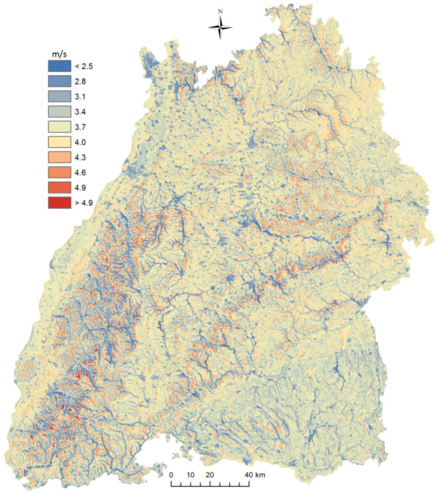
2.1. Study Area and Wind Speed Measurements

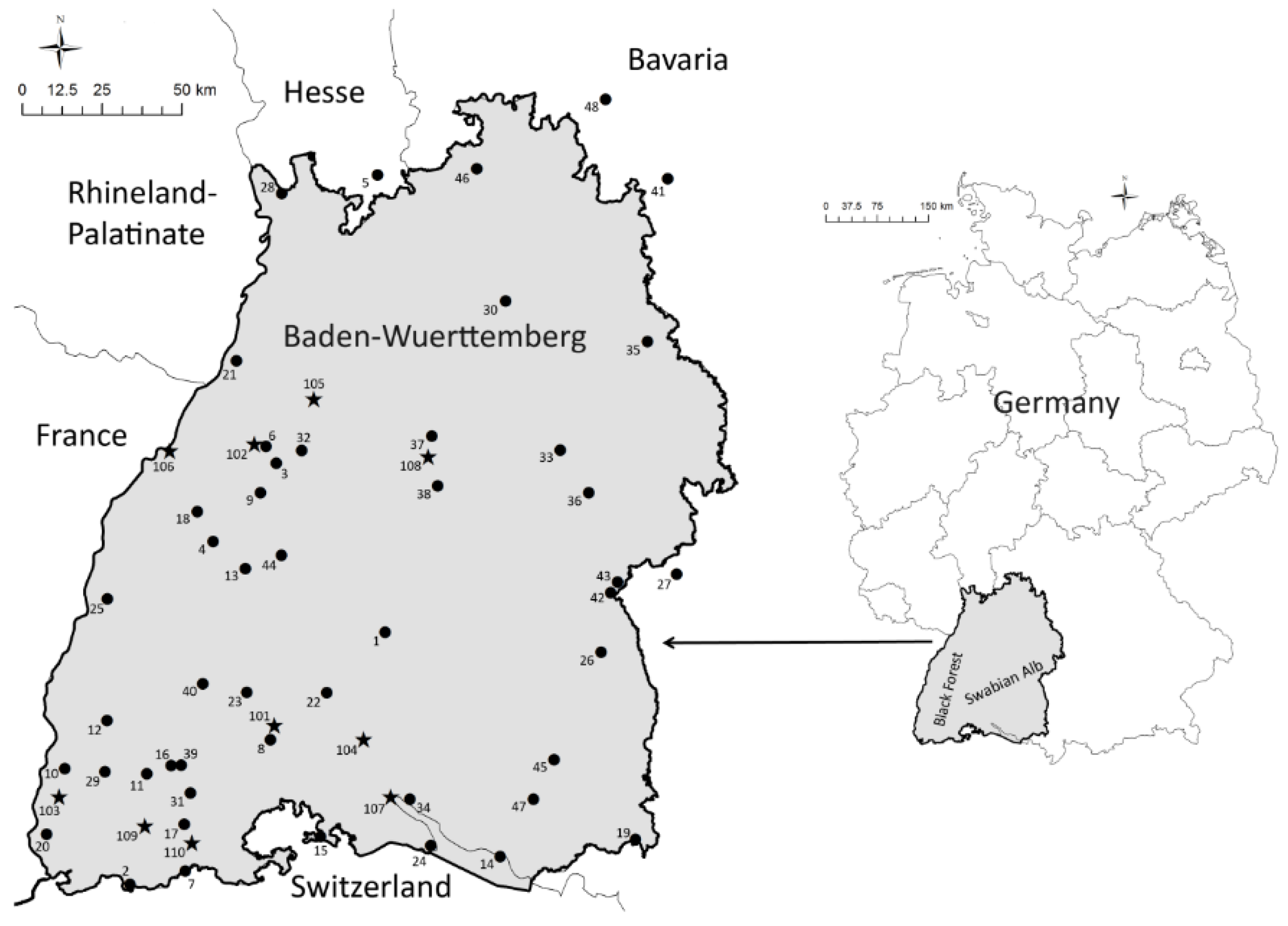
The study area is the German federal state of Baden-Wuerttemberg (Figure 1). The low mountain ranges Black Forest (length ~150 km, width ~30–50 km, highest elevations >1400 m) and Swabian Alb (length ~180 km, width ~35 km, highest elevations >1000 m) are the most complex topographical features with the strongest impact on the wind resource over the study area [20]. The top of the Feldberg (1493 m) is the highest elevation in the study area. Approximately 38% (13,700 km²) of the study area is covered with forests [21]. More details about land cover and topographical features in the study area are summarized in [20].

The wind speed database used in this study consists of time series of the daily mean wind speed measured from 1 January 1979 to 31 December 2010 at 58 meteorological stations by the German Weather Service (DWD). The height (h_S) of wind speed measurements varies between 3 m AGL (stations Bad Wildbad-Sommerberg, Isny) and 48 m AGL (station Karlsruhe). Data preparation included gap filling, testing for homogeneity and detrending according to [20].

The median wind speed near the surface values (${\tilde{U}}_{\mathrm{s}}$) vary in the range 0.5 m/s (station Triberg) to 7.5 m/s (station Feldberg) (

Table 1. List of DWD stations and corresponding data features. DS1 stations are indicated by identification numbers (ID) 1–48; DS2 stations are indicated by ID values 101–110. ${\tilde{U}}_{\mathrm{s}}$: median wind speed near the surface values; h_S: height.

ID	Station	${\tilde{U}}_{\mathrm{s}}$	hs	ID	Station	${\tilde{U}}_{\mathrm{s}}$	hs
1	Albstadt-Onstmettingen	1.7	17	30	Öhringen	2.3	16
2	Bad Säckingen	0.9	10	31	Schluchsee	1.6	10
3	Bad Wildbad-Sommerberg	0.7	3	32	Schömberg	0.6	10
4	Baiersbronn-Obertal	0.9	10	33	Schwäbisch-Gmünd	0.7	10
5	Beerfelden	1.7	10	34	Sipplingen	2.5	16
6	Dobel	2.3	10	35	Stimpfach-Weiptershofen	2.1	10
7	Dogern	1.7	10	36	Stötten	4.1	12
8	Donaueschingen	2.5	10	37	Stuttgart (Schnarrenberg)	2.5	12
9	Enzklösterle	1.0	10	38	Stuttgart-Echterdingen	2.5	10
10	Eschbach	2.4	10	39	Titisee	0.7	11
11	Feldberg	7.5	19	40	Triberg	0.5	15
12	Freiburg	2.4	12	41	Uffenheim	1.3	10
13	Freudenstadt	3.7	34	42	Ulm	2.2	10
14	Friedrichshafen	3.1	10	43	Ulm-Wilhelmsburg	2.7	15
15	Gailingen	1.6	12	44	Waldachtal-Lützenhardt	1.2	6
16	Hinterzarten	1.2	6	45	Waldsee, Bad-Reute	2.2	10
17	Höchenschwand	1.2	6	46	Walldürn	2.9	10
18	Hornisgrinde	5.9	10	47	Weingarten	1.9	12
19	Isny	2.1	3	48	Würzburg	2.8	12
20	Kandern-Gupf	2.0	10	101	Bad Dürrheim	1.3	10
21	Karlsruhe	3.3	48	102	Bad Herrenalb	0.6	10
22	Klippeneck	3.9	16	103	Müllheim	1.3	6
23	Königsfeld	1.0	6	104	Neuhausen ob Eck	2.5	10
24	Konstanz	1.7	17	105	Pforzheim-Ispringen	2.6	12
25	Lahr	2.3	10	106	Söllingen	2.6	10
26	Laupheim	2.5	10	107	Stockach-Espasingen	1.5	12
27	Leipheim	2.3	10	108	Stuttgart-Stadt	1.7	26
28	Mannheim	2.7	22	109	Todtmoos	1.1	10
29	Münstertal	1.3	10	110	Weilheim-Bierbronnen	2.6	10

). To extend the database, four measurement stations located in the bordering federal states Hesse and Bavaria were included in this study. Out of the 58 wind speed time series, 48 time series were put into a parameterization dataset (DS1). The remaining 10 time series, for which the original length was less than 10 years, belong to the validation dataset (DS2).

2.2. Wind Speed Extrapolation

All wind speed near the surface (U_S) time series were extrapolated to 100 m AGL using the Hellman power law [22,23,24]. It was demonstrated by [11] that the power law performs well compared to similar wind speed extrapolation methods. According to [22], the accuracy of the power law increases when stratification effects and the influence of the wind speed are considered. Therefore, the Hellmann exponent (E) was computed on a daily basis.

As has previously been done by [20,25], daily mean wind speed at the 850 hPa pressure level (U_850hPa) and the height of the 850 hPa pressure level AGL (h_850hPa), both available from the European Centre for Medium-Range Weather Forecast [26], were used to calculate daily, station-specific E-values:

$$E=\frac{\text{ln}\left(\frac{U_{\text{850hPa}}}{U_s}\right)}{\text{ln}\left(\frac{h_{\text{850hPa}}}{h_s}\right)}$$

(1)

After the E-values were determined, daily, station-specific U_S-values were extrapolated to 100 m AGL yielding U_100m,emp:

$$U_{\text{100m,emp}}=U_s\times {\left(\frac{100m}{h_s}\right)}^E$$

(2)

2.3. Probability Distribution Fitting

Prior to the probability distribution fitting, U_100m,emp time series were transformed to empirical cumulative distribution functions (CDF_emp). Afterwards, 67 CDF were fitted to each CDF_emp. The goodness of fit (GoF) of each CDF was quantified by calculating the coefficient of determination (R²) from probability plots [19,27] and the Kolmogorov-Smirnov statistic (D) [28,29,30] to the fits. The D-values were obtained by measuring the largest vertical difference between CDF and CDF_emp. The transformation of time series, fitting and GoF evaluation were done by EasyFit software (Version 5.5, MathWave Technologies, Dnepropetrovsk, Ukraine) and Matlab^® Software Optimization Toolbox (Release 2015a; The Math Works Inc., Natick, MA, USA).

According to D- and R²-value evaluation, which will be presented in detail in the results section, the five-parameter Wakeby distribution (WK5) [31] is clearly the best-fitting distribution. It can be defined by its quantile function [20,25,31,32]:

$$U_{\text{100m,distr}}(F)=\mathsf{\epsilon }+\frac{\mathsf{\alpha }}{\mathsf{\beta }}\times \left[1-{\left(1-F\right)}^{\mathsf{\beta }}\right]-\frac{\mathsf{\gamma }}{\mathsf{\delta }}\times \left[1-{\left(1-F\right)}^{-\mathsf{\delta }}\right]$$

(3)

where F is the cumulative probability with U_100m,distr (F) being the associated wind speed value. The four parameters α, β, γ, and δ are distribution parameters and the fifth parameter, ε, is the location parameter. WK5 can be interpreted as a mixed distribution [33] consisting of a left and right part [31,32]. This enables WK5 to reproduce shapes of wind speed distributions that other distributions cannot reproduce [25,31].

2.4. Predictor Variable Building

A total number of 92 predictor variables (50 m × 50 m) covering the study area were built by using the ArcGIS^® 10.2 software (Esri, Redlands, CA, USA). All predictor variables originate from a digital terrain model (DTM), CORINE Land Cover (CLC) data [34] or ERA-Interim reanalysis U_850hPa [26].

The DTM was used to map Φ, τ [35,36], curvature, aspect and slope. The Φ-values were calculated by subtracting the mean elevation of an outer circle around each grid point from the grid point-specific elevation. Five different Φ variants with outer-circle radii of 250 m, 500 m, 1000 m (Φ_1000m), 2500 m (Φ_2500m) and 5000 m (Φ_5000m) were created.

The τ-maps were built for eight main compass directions (northeast (22.5°–67.4°), east (67.5°–112.4°), southeast (112.5°–157.4°), south (157.5°–202.4°), southwest (202.5°–247.4°), west (247.5°–292.4°), northwest (292.5°–337.4°), north(337.5°–22.4°)) at 200 m radius intervals. This was done by summing angles up to a distance limited to 1000 m. Curvature, aspect and slope were calculated by using the Spatial Analyst Toolbox in ArcGIS.

Roughness length (z₀) was derived from CLC data with an original spatial resolution of 100 m × 100 m. Roughness length values were assigned to land cover types according to [20] yielding the local roughness length (z_0,l). Additionally, “effective” roughness length values (z_0,eff) for the eight main compass directions were calculated. This was done for four different radii around each grid point (100 m, 200 m, 300 m, 400 m). In the end, all z₀-values were interpolated to 50 m × 50 m resolution grids.

U_850hPa data (0.125° × 0.125° resolution) were included into model building because it represents large-scale airflow undisturbed by the surface [37]. The 0.01, 0.30, 0.50, 0.75 and 0.99 percentiles of U_850hPa time series covering the period from 01 January 1979 to 31 December 2010 were calculated (U_850hPa,0.01, U_850hPa,0.30, U_850hPa,0.50, U_850hPa,0.75 and U_850hPa,0.99) and mapped in ArcGIS®. A spline interpolation was applied to convert the U_850hPa layers to 50 m × 50 m resolution grids.

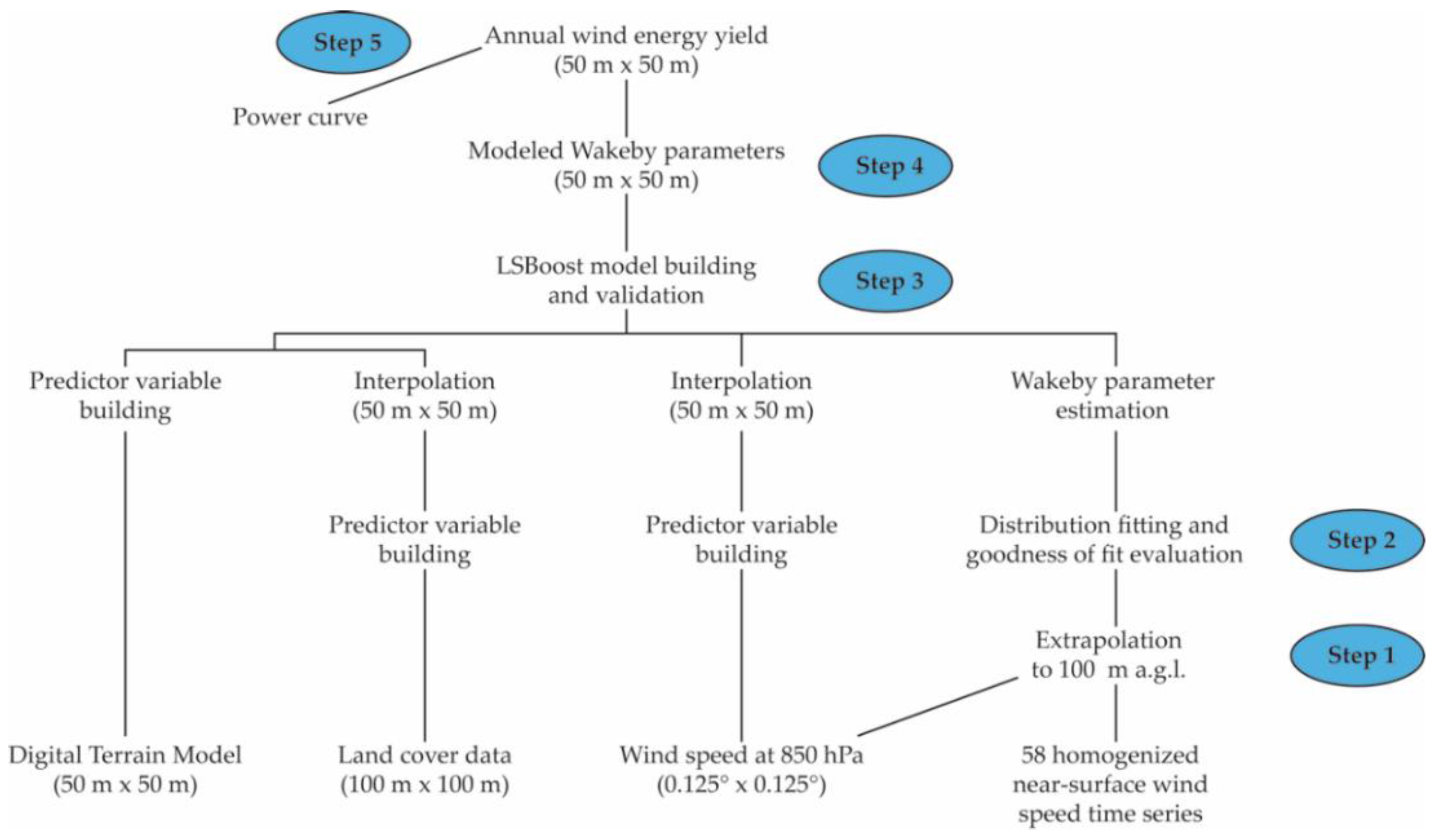
2.5. Wakeby Parameter Estimation and Modeling

The procedure applied to obtain the Wakeby parameters at every grid point in the study area comprised the following work steps: (1) estimating the Wakeby parameters of every CDF_emp based on L-moments [38,39]; (2) analyzing the obtained Wakeby parameters and identifying common characteristics of all distributions ; and (3) modeling target variables (Y) that enable the calculation of all WK5 parameters at every grid point in the study area. To make the WK5 parameter modeling more robust, the WK5 parameters estimated by L-moments were modeled indirectly according to [20,25].

Analyzing the estimated distributions led to the following parameter modeling and calculation approach: First, the estimated left-hand tail of WK5 (Y_L), which is represented by α, β and ε, was modeled:

$$Y_{\mathrm{L}}=\mathsf{\epsilon }+\frac{10}{\mathsf{\beta }}\times \left[1-{\left(1-0.25\right)}^{\mathsf{\beta }}\right]$$

(5)

The estimated location parameter ε, which represents the lower bound of the distribution, was directly modeled. Because the L-moment-based WK5 parameter estimation showed that α = 10 at nearly all stations, it was set to this value. The use of a fixed α-value enabled the subsequent calculation of β.

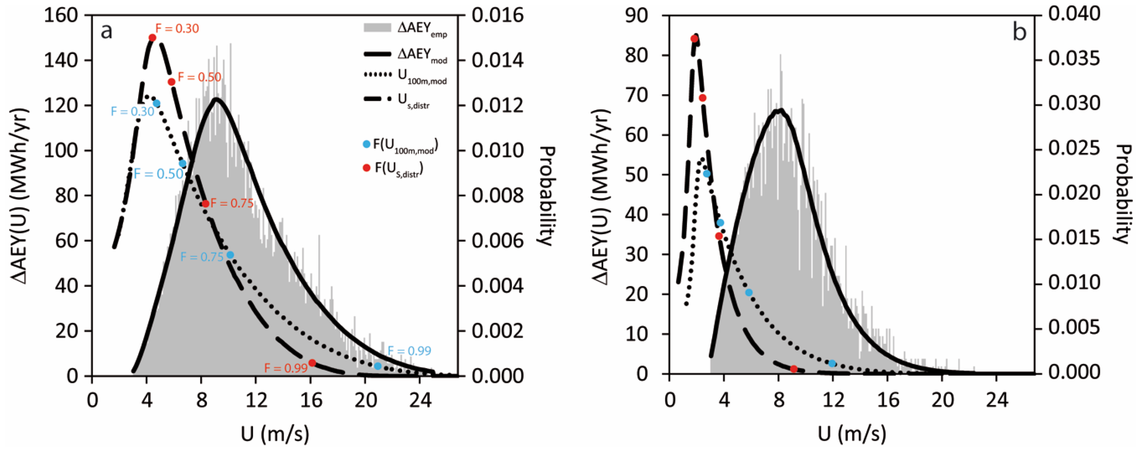
Since Y_L affected WK5 parameter estimation up to F = 0.25, exactly as described by [31,32], the percentiles F = 0.30 (Y_R1), F = 0.50 (Y_R2), F = 0.75 (Y_R3) and F = 0.99 (Y_R4) were modeled to build the right-hand tail of WK5 (Y_R). A system of non-linear equations was solved at every grid point yielding γ and δ:

$$\{\begin{array}{l}\frac{\mathsf{\gamma }}{\mathsf{\delta }}\times \left[1-{\left(1-0.30\right)}^{-\mathsf{\delta }}\right]+\left[Y_{\text{R1}}-Y_{\mathrm{L}}\right]=0\\ \frac{\mathsf{\gamma }}{\mathsf{\delta }}\times \left[1-{\left(1-0.50\right)}^{-\mathsf{\delta }}\right]+\left[Y_{\text{R2}}-Y_{\mathrm{L}}\right]=0\\ \frac{\mathsf{\gamma }}{\mathsf{\delta }}\times \left[1-{\left(1-0.75\right)}^{-\mathsf{\delta }}\right]+\left[Y_{\text{R3}}-Y_{\mathrm{L}}\right]=0\\ \frac{\mathsf{\gamma }}{\mathsf{\delta }}\times \left[1-{\left(1-0.99\right)}^{-\mathsf{\delta }}\right]+\left[Y_{\text{R4}}-Y_{\mathrm{L}}\right]=0\end{array}$$

(6)

In order to calculate U_100m,mod, Y_L and Y_R were recombined yielding WK5 with modeled parameters (WK5_mod).

All Y were computed for every grid point by least squares boosting (LSBoost) [40]. This was done by using the Ensemble Learning algorithm LSBoost implemented in the Matlab® Software Statistics Toolbox (Release 2015a; The Math Works Inc.). LSBoost is basically a sequence of simple regression trees, which are called weak learners (B). The objective of LSBoost is to minimize the mean squared error (MSE) between Y and the aggregated prediction of the weak learners (Y_pred). In the beginning, the median of the target variables ($\tilde{Y}$) is calculated. Afterwards, multiple regression trees B₁, …, B_m are combined in a weighted manner [41] to improve model accuracy. The individual regression trees are a function of selected predictor variables (X):

$$Y_{\text{pred}}\left(X\right)=\tilde{Y}\left(X\right)+\nu {\displaystyle \sum _{m=1}^M{p}_m\times }{B}_m\left(X\right)$$

(4)

with p_m being the weight for model m, M is the total number of weak learners, and v with 0 < v ≤ 1 is the learning rate [20,41].

The predictor variable selection process comprised several steps. First, the most appropriate length of outer-circle radii for τ and z_0,eff were determined by the correlation coefficient (r) between τ respectively z_0,eff and Y. Secondly, the importance of the remaining predictor variables was evaluated by predictor importance (PI) which quantifies the relative contribution of individual predictor variables to the model output [21]. The PI-values were determined by summing up changes in MSE due to splits on every predictor and dividing the sum by the number of branch nodes. All predictor variables with PI = 0.00 were sorted out.

After PI-evaluation, combinations of predictor variables were tested for their predictive power. Starting with one predictor variable, further predictor variables were added to the model and kept when the model accuracy measures R², mean error (ME), mean absolute error (MAE), MSE and mean absolute percentage error (MAPE) improved [42,43,44]. For model parameterization, DS1 data were used. Model validation was done with both DS1 and DS2 data.

Multicollinearity among the predictor variables was investigated by assessing the variance inflation and the condition index in combination with variance decomposition proportions according to [45].

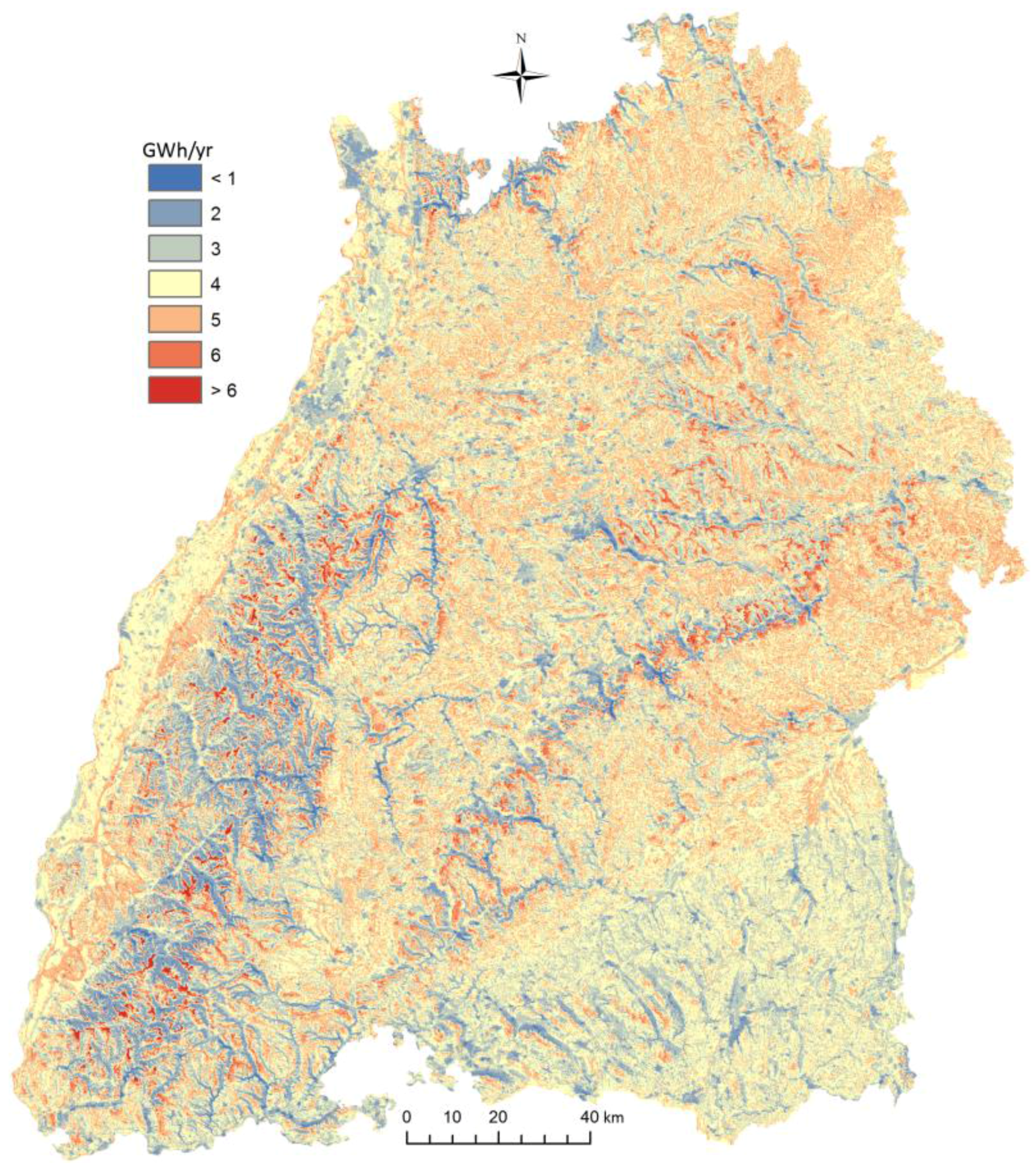
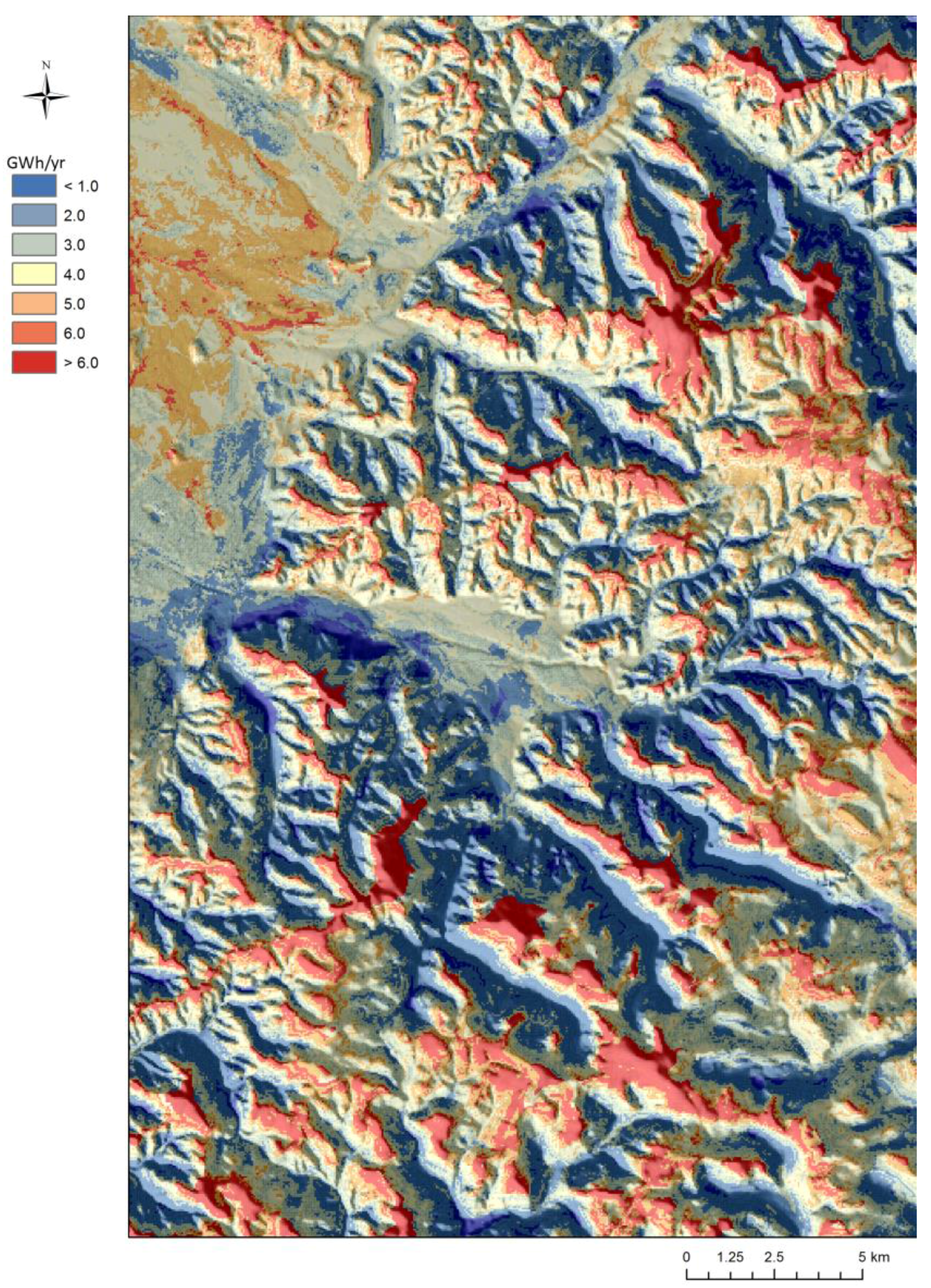
2.6. Annual Wind Energy Yield Estimation

The relationship between wind speed and the electrical power output (P) of wind turbines is typically established by a power curve [46]. Power curve values are developed from field measurements and can be used for studies involving energy calculations [47]. There are three important points characterizing a typical power curve (Figure 2): (1) at the cut-in speed the wind turbine starts to generate usable power; (2) after exceeding the rated output speed the maximum output power (rated power) is generated; and (3) after exceeding the cut-out speed turbines cease power generation and shut down [46]. A standard 2.5 MW power curve [48] for onshore wind power plants was applied to calculate the AEY.

The discrete P-values from the manufacturer power curve were interpolated by a spline to obtain a continuous power curve. The basic attributes of the applied power curve are: cut-in speed U_100m = 3.0 m/s; cut-out speed U_100m = 25.0 m/s; rated output speed U_100m = 13.0 m/s and; rated output power P = 2580 kW. The empirical annual wind energy yield (AEY_emp) was calculated for each station in DS1 and DS2 following [49]:

$$AE{Y}_{\text{emp}}=({\displaystyle \sum _{i=1}^{N}P(U_{\text{100m,emp,i}}})/Z_1$$

(7)

with N = 11,688 being the total number of days in the investigation period and the number of years in the investigation period (Z₁).

The average electrical power output ($\overline{P}$) was calculated according to [19,50]:

$$\overline{P}={\displaystyle \underset{0}{\overset{\infty }{\int }}P(U_{\text{100m,mod}})\times f(U_{\text{100m,mod}})}\mathrm{d}{U}_{\text{100m,mod}}$$

(8)

The above equation describes the electrical power produced at each wind speed class multiplied by the probability of the specified wind speed class and integrated over all possible wind speed classes [50] with f(U_100m,mod) being the probability density of U_100m,mod. After $\overline{P}$ is calculated modeled annual wind energy yield (AEY_mod) can be computed by multiplying $\overline{P}$ with the respective number of days per year (Z₂):

$$AE{Y}_{\text{mod}}=\overline{P}\times Z_2$$

(9)

2.7. Summary of the Methodology

The methodology for the quantification of AEY in the study area is summarized in Figure 3. The basic steps are:

(1)

Extrapolation of near-surface wind speed time series to hub height;

(2)

Identification of a theoretical distribution that is capable of reproducing various shapes of empirical wind speed distributions;

(3)

Modeling the estimated parameters of the identified theoretical distribution, based on large-scale airflow, surface roughness and topographic features;

(4)

Mapping of distribution parameters in the study area; and

(5)

Calculation of the AEY using a wind turbine-specific power curve.

3. Results and Discussion

3.1. Distribution Fitting

According to results from the D-evaluation, WK5 fits 23 CDF_emp best. As can be seen in

Table 2. Distributions ranked (RK) by Kolmogorov-Smirnov statistic (D)-values with their number of parameters (NP). D- and coefficient of determination (R²)-values are averages over all meteorological stations.

RK	Distribution	D	R2	NP	RK	Distribution	D	R2	NP
1	Wakeby	0.02	0.9992	5	35	Weibull	0.10	0.9768	2
2	Johnson SB	0.03	0.9991	4	36	Pert	0.11	0.9732	3
3	Inv. Gaussian	0.03	0.9981	3	37	Rayleigh	0.12	0.9721	2
4	Pearson 6	0.03	0.9984	4	38	Erlang	0.12	0.9866	3
5	Pearson 6	0.03	0.9983	3	39	Normal	0.13	0.9492	2
6	Lognormal	0.03	0.9982	3	40	Rice	0.13	0.9653	2
7	Dagum	0.03	0.9978	3	41	Logistic	0.13	0.9511	2
8	Fatigue Life	0.03	0.9978	3	42	Hypersecant	0.14	0.9497	2
9	Gen. Extreme	0.04	0.9975	3	43	Uniform	0.14	0.9351	2
10	Burr	0.04	0.9974	4	44	Cauchy	0.15	0.9845	2
11	Log-Logistic	0.04	0.9971	3	45	Erlang	0.15	0.9909	2
12	Burr	0.04	0.9971	3	46	Chi-Squared	0.16	0.9908	2
13	Lognormal	0.04	0.9973	2	47	Error	0.16	0.9437	3
14	Bimodal Weibull	0.04	0.9985	5	48	Laplace	0.17	0.9412	2
15	Fatigue Life	0.04	0.9970	2	49	Chi-Squared	0.19	0.9920	1
16	Inv. Gaussian	0.04	0.9974	2	50	Gumbel Min	0.20	0.8976	2
17	Pearson 5	0.04	0.9958	3	51	Exponential	0.23	0.9863	2
18	Bimodal Normal	0.04	0.9956	5	52	Exponential	0.27	0.9833	1
19	Gen. Pareto	0.04	0.9976	3	53	Pareto 2	0.28	0.9841	2
20	Gen. Gamma	0.04	0.9954	4	54	Triangular	0.31	0.9132	3
21	Dagum	0.04	0.9957	4	55	Power Func.	0.31	0.9138	3
22	Pearson 5	0.05	0.9954	2	56	Levy	0.36	0.9777	2
23	Gen. Logistic	0.05	0.9947	3	57	Levy	0.39	0.9769	1
24	Log-Logistic	0.05	0.9952	2	58	Error Func.	0.70	0.9103	1
25	Gamma	0.06	0.9931	3	59	Student’s t	0.82	0.7991	1
26	Beta	0.06	0.9922	4	-	Johnson SU	No Fit		4
27	Gen. Gamma	0.06	0.9904	3	-	Log-Gamma	No Fit		2
28	Gamma	0.06	0.9910	2	-	Log-Pearson 3	No Fit		3
29	Frechet	0.06	0.9909	3	-	Nakagami	No Fit		2
30	Gumbel Max	0.07	0.9879	2	-	Pareto	No Fit		2
31	Weibull	0.07	0.9851	3	-	Reciprocal	No Fit		2
32	Frechet	0.07	0.9892	2	-	Phased Bi-Exp.	No Fit		4
33	Kumuaraswamy	0.09	0.9805	4	-	Phased Bi-Wei.	No Fit		6
34	Rayleigh	0.10	0.9776	1	-	-	-		-

, the D-value averaged over all stations for WK5 (0.02) is lower than the average D-value of all other theoretical distributions. Another well-fitting distribution is the four-parameter Johnson SB distribution (D = 0.03). The best fitting three-parameter distribution is the inverse Gaussian distribution (D = 0.03). In general, the performance of theoretical distributions defined by three or more parameters is better than the performance of two- and one-parameter distributions. In the case of eight theoretical distributions (Johnson SU, Log-Gamma, Log-Pearson 3, Nakagami, Pareto, Reciprocal, Phased Bi-Exponential, Phased Bi-Weibull) no fit to CDF_emp could be achieved and therefore the parameter estimation procedure failed.

A widely used theoretical distribution applied to empirical wind speed distributions is the two-parameter Weibull distribution [30,51,52,53,54,55,56,57,58]. However, in this study, the fit of the Weibull distribution is poor (D = 0.10) compared to many other theoretical distributions. These results are in accordance with similar studies where the GoF of various theoretical distributions to empirical distributions was compared [59,60,61]. The Weibull distribution is not even the best-fitting two-parameter distribution, which is the lognormal distribution. The best GoF of a one-parameter distribution was achieved by the also widely used Rayleigh distribution [62,63]. However, compared to many distributions defined by more parameters the GoF of the Rayleigh distribution was rather poor (D = 0.10). An explanation for the poor fit of distributions with less than three parameters might be that their capacity for reproducing irregular shapes of empirical distributions is limited. Irregularly shaped empirical wind speed distributions often result from complex topography [64].

The evaluation of averaged R²-values confirms results of the D-values evaluation. The best-fitting distribution is WK5 (R² = 0.9992), followed by Johnson SB (R² = 0.9991).

The superior fit of WK5 is in accordance to GoF measures of empirical near-surface (10 m AGL) wind speed distributions in the study area [20]. Based on the results presented in this study it is concluded that WK5 is a universal wind speed distribution for the study area.

3.2. Predictor Variable Selection and Importance

The screening of r-values showed that the most appropriate length of outer-circle radius was 1000 m for τ and 200 m for z_0eff.

Table 3. Relative importance of predictor variables used for final least squares boosting models (LSBM) in percent. The top three important predictor variables are highlighted in red.

ID	Predictor variable	Symbol	YL	ε	YR1	YR2	YR3	YR4
1	Wind speed at 850 hPa level (F = 0.75)	U850hPa,0.75	-	-	-	-	$21.4$	-
2	Wind speed at 850 hPa level (F = 0.99)	U850hPa,0.99	-	-	-	-	-	$14.8$
3	Roughness length, local	z0,l	$1.9$	0.1	0.4	-	-	1.5
4	Roughness length, effective, W	z0eff,W	-	-	-	$9.2$	-	-
5	Roughness length, effective, SW	z0eff,SW	-	-	0.6	-	-	-
6	Roughness length, effective, S	z0eff,S	-	-	$7.8$	2.2	1.5	6.2
7	Roughness length, effective, N	z0eff,N	-	-	1.1	-	6.9	-
8	Topographic exposure, NW	τNW	-	-	-	$9.8$	-	5.2
9	Topographic exposure, W	τW	-	$21.4$	-	-	-	$20.8$
10	Topographic exposure, SW	τSW	$24.4$	$23.5$	$9.6$	-	$20.8$	-
11	Topographic exposure, SE	τSE	-	-	-	-	-	2.4
12	Relative elevation, 1000 m	Φ1000m	$73.7$	$55.0$	-	-	$49.4$	-
13	Relative elevation, 2500 m	Φ2500m	-	-	$80.5$	-	-	-
14	Relative elevation, 5000 m	Φ5000m	-	-	-	$78.8$	-	$49.1$

lists the predictor variables used for all six least squares boosting models (LSBM) and their relative impact to the model outputs. From the large set of predictor variables, predictor selection finally reduced their number to 14.

The main wind directions in the study area are west and southwest. It is therefore reasonable that southwesterly and westerly oriented τ- and z_0eff-predictor variables have a distinct impact to the model outputs. The highest PI-values for any roughness length predictor variable are found for the LSBM output Y_R2 and the western sector (PI = 9.2%). However, the PI-value for Y_R1 and the southwestern sector is relatively low (PI = 0.6%). The topographic exposure for the southwestern sector, respectively the western sector, is one of the most important predictor variables for modeling ε, Y_L, Y_R3 and Y_R4.

It is important to note that U_850hPa was not used to model the left-hand tail of WK5, which represents U_100m,mod-values. Low wind speed values mostly occur when the atmosphere is stably stratified [22]. Thus, the influence of U_850hPa on U_100m,mod is rather small.

When modeling Y_R3 and Y_R4, the large-scale airflow becomes more important PI = {21.4%, 14.8%} because high U_100m,mod-values usually occur when the atmosphere is neutrally stratified [22].

Results from PI-evaluation indicate the fundamental role of relative elevation in wind turbine site assessment. The high PI-values for Φ indicate the great importance of Φ for model outputs. The highest PI-value is 80.5% for Φ_2500m when modeling Y_R1. In contrast, the absolute elevation (ψ) was never used as predictor variable. This is reasonable because sites with high ψ-values are not necessarily exposed to high wind speeds.

3.3. Wind Speed Mapping

Median U_100m,mod-values (${\tilde{U}}_{\text{100m,mod}}$) are shown in Figure 4. In large parts (75%) of the study area, ${\tilde{U}}_{\text{100m,mod}}$-values are in the range between 3.0 m/s and 4.0 m/s. In only 0.2% of the study area, ${\tilde{U}}_{\text{100m,mod}}$-values are above 4.9 m/s. Due to the complex topography, high and low ${\tilde{U}}_{\text{100m,mod}}$-values can occur within small distances (<500 m). For example, in the Black Forest, which is characterized by narrow, forested valleys, ${\tilde{U}}_{\text{100m,mod}}$-values are very low. However, there are many exposed mountaintops in close proximity to these valleys where ${\tilde{U}}_{\text{100m,mod}}$-values are high. Beside narrow, forested valleys, lowest ${\tilde{U}}_{\text{100m,mod}}$-values (<3.1 m/s) occur in large cities. In the entire study area the effect of topographic exposure on the modeling results is evident by predominantly higher ${\tilde{U}}_{\text{100m,mod}}$-values at sites exposed to the West and Southwest.

3.4. Annual Wind Energy Yield

In Figure 5, the empirical AEY per wind speed class (ΔAEY_emp), the modeled AEY per wind speed class (ΔAEY_mod), the probability density distributions of WK5_mod and the probability density distributions fitted to U_S-values (U_S,distr) are presented as a function of wind speed classes (intervals of 0.1 m/s) for the stations Hornisgrinde (Figure 5a) and Laupheim (Figure 5b).

It is clear that percentiles (F = {0.30–0.99}) from the right-hand tail of WK5_mod contribute more to AEY and are thus more important for the total amount of AEY_mod. In Laupheim the mode of U_100,mod is 2.3 m/s, whereas highest ΔAEY_mod is obtained at 8.0–8.1 m/s. Even at the top of the Hornisgrinde, which is one of the windiest places in the study area, the U_100m,mod mode value at 4.2 m/s is clearly lower than the wind speed class assigned to the highest ΔAEY_mod-value (9.0–9.1 m/s). Overall, the ΔAEY_mod-curves fit ΔAEY_emp-values obtained for both stations well.

The map of AEY_mod (Figure 6) shows similar patterns like the ${\tilde{U}}_{\text{100m,mod}}$-map. By applying the power curve to U_100m,mod, the mean AEY_mod-value in the study area is 3.4 GWh/yr. The highest AEY_mod-value (13.6 GWh/yr) occurs at the top of the Feldberg. Only in 3% of the study area is AEY_mod higher than 5.0 GWh/yr. In 31% of the study area AEY_mod is lower than 3.0 GWh/yr with a tendency towards lower AEY_mod-values in the southeast, which is mainly due to low U_850hPa-values in this part over the study area. In contrast, generally higher AEY_mod-values were calculated in the northeast where U_850hPa-values are highest at the landscape level. The spatial AEY_mod-pattern indicates that the local wind resource is mainly determined by terrain features and surface roughness.

This is underlined by the map extract shown in Figure 7. In the topographically structured Black Forest region, it appears that highest and lowest AEY_mod-values occur over horizontal distances shorter than 500 m. This finding is in good accordance to a previous study regarding gust speed in the same area [25]. The main wind direction can be inferred from highest AEY_mod-values over southwest-facing slopes.

Figure 8 shows r-values which were calculated between AEY_mod and various predictor variables. The r-values confirm the results of the PI-evaluation. The highest and lowest r-values are obtained for the most important predictor variables. The highest absolute r-values are (r = |−0.59|) for τ_SW and (r = |0.58|) for Φ_2500m. The correlation between ψ and AEY_mod is relatively weak (r = 0.08). This is due to the fact that some highly elevated Black Forest valleys are sites with the lowest AEY_mod-values. The correlation between U_850hPa,0.75 and AEY_mod (r = 0.08) is also relatively low since the influence of the large-scale airflow on AEY_mod is superimposed by influences of local terrain features and surface roughness. All correlations are highly significant with significance values (p) p ≤ 0.0000.

The exemplary functional relationships between classes of four important predictor variables and AEY_mod are shown in Figure 9. The variability of AEY_mod-values as a function of U_850hPa,0.75 (Figure 9a) is lower than the variability of the other displayed predictor variables. This is interpreted to mean that the variability of U_850hPa,0.75 is of minor importance for explaining the spatial AEY_mod-patterns in the study area. Due to their high roughness, AEY_mod is lower over forests and cities (Figure 9b). Areas that are exposed to the southwest (τ_SW < 2°) show higher AEY_mod-values (median: 3.9 GWh/yr) than sheltered areas (τ_SW > 18°) (median: 1.5 GWh/yr) (Figure 9c). The strongest functional relationship is between Φ_2500m and AEY_mod (Figure 9d). The assigned median AEY_mod-values increase from 1.6 GWh/yr at Φ_2500m < −150 m to 4.7 GWh/yr at Φ_2500m > 150 m.

3.5. Model Validation

The MAPE-values indicate that U_100m,mod was simulated accurately (

Table 4. Performance measures coefficient of determination (R²), mean error (ME), mean absolute error (MAE), mean squared error (MSE) and mean absolute percentage error (MAPE) calculated from the comparison of empirical and modeled cumulative probabilities (F) associated with U_100m-time series included in DS1 and DS2.

Data Set	F	R2	ME (m/s)	MAE (m/s)	MSE (m/s)	MAPE (%)
DS1	0.10	0.97	0.05	0.11	0.02	5.9
	0.20	0.97	0.04	0.11	0.02	5.1
	0.30	0.97	0.01	0.12	0.02	4.6
	0.40	0.97	0.00	0.13	0.03	4.3
	0.50	0.97	0.00	0.14	0.03	4.2
	0.60	0.97	−0.01	0.16	0.04	4.1
	0.70	0.97	−0.01	0.20	0.06	4.2
	0.80	0.97	−0.01	0.25	0.09	4.3
	0.90	0.97	−0.09	0.33	0.17	4.6
	0.99	0.98	0.00	0.38	0.23	3.2
Data Set	F	R2	ME (m/s)	MAE (m/s)	MSE (m/s)	MAPE (%)
DS2	0.10	0.95	−0.01	0.07	0.01	3.6
	0.20	0.95	−0.03	0.10	0.01	4.5
	0.30	0.96	−0.06	0.10	0.02	4.0
	0.40	0.97	−0.07	0.12	0.02	4.3
	0.50	0.97	−0.07	0.14	0.02	4.4
	0.60	0.96	−0.08	0.17	0.04	4.7
	0.70	0.95	−0.10	0.21	0.07	5.0
	0.80	0.95	−0.12	0.25	0.10	5.1
	0.90	0.95	−0.24	0.36	0.17	5.5
	0.99	0.94	−0.30	0.46	0.42	4.0

). They are always below 6% for both DS1 and DS2. The R²-values are mostly 0.97 for DS1 percentiles and about 0.95 for DS2 percentiles. The largest downward bias is ME = −0.30 m/s for F = 0.99.

The model performance for DS2 is only marginally worse than for DS1. This indicates the portability of LSBM to other data sets.

Performance measures from the comparison of modeled cumulative distribution functions (CDF_mod) with CDF_emp associated with U_100m-time series included in DS2 are shown in

Table 5. Performance measures from the comparison of modeled cumulative distribution function (CDF_mod) with empirical cumulative distribution function (CDF_emp) associated with U_100m time series included in DS2.

Station	D	R2	Station	D	R2
Bad Dürrheim	0.05	0.9977	Söllingen	0.06	0.9973
Bad Herrenalb	0.05	0.9973	Stockach-Espasingen	0.08	0.9918
Müllheim	0.05	0.9982	Stuttgart-Stadt	0.09	0.9924
Neuhausen ob Eck	0.02	1.0000	Todtmoos	0.07	0.9968
Pforzheim-Ispringen	0.04	0.9991	Weilheim-Bierbronnen	0.06	0.9978

.

It appears that the GoF measures for modeled WK5 parameters are better than for many statistical distributions that were directly fitted to CDF_emp (compare Table 2).

In Figure 10, AEY_emp is plotted against AEY_mod. Related performance measures for DS1 (Figure 10a) and DS2 (Figure 10b) are R² = {0.98, 0.97}, ME = {−0.16 GWh/yr, −0.23 GWh/yr}, MAE = {0.32 GWh/yr, 0.31 GWh/yr}, MSE = {0.16 GWh/yr, 0.13 GWh/yr} and MAPE = {10.0%, 17.1%}. Thus, it can be concluded that the calculated AEY_emp-values were modeled with sufficient accuracy.

4. Conclusions

A methodology is presented that allows assessing the statistical AEY on a high spatial resolution (50 m × 50 m) grid in an area with mosaic-like land cover pattern and complex topography. It was found that highest and lowest AEY occurs in highly textured terrain within very small distances (<500 m). The results of this study therefore emphasize the need to assess AEY at very small spatial scales. This is demonstrated in particular by the great importance of the predictor variables relative elevation and topographic exposure in the main wind direction.

Since the methodology allows for the calculation of all WK5 parameters, the AEY for any manufacturer power curve can be estimated. The methodology is easily portable to other heights above ground level as well as to other study areas. The only requirements for the portability are the availability of the following: (i) near-surface wind speed time series as measured in meteorological networks; (ii) a DTM; (iii) a land cover data set; and (iv) wind speed data not influenced by local topography or land use.

The proposed modeling approach is a useful first step in the exploration of the most appropriate wind turbine sites based on the local wind resource. The produced model outputs and maps are valuable starting points for further in-depth wind turbine site assessment.

References

1. Kaldellis, J.K.; Zafirakis, D. The wind energy (r) evolution: A short review of a long history. Renew. Energy 2011, 36, 1887–1901. [Google Scholar] [CrossRef]
2. Leung, D.Y.; Yang, Y. Wind energy development and its environmental impact: A review. Renew. Sustain. Energy Rev. 2012, 16, 1031–1039. [Google Scholar] [CrossRef]
3. Lew, D.J. Alternatives to coal and candles: Wind power in China. Energy Policy 2000, 28, 271–286. [Google Scholar] [CrossRef]
4. Büsgen, U.; Dürrschmidt, W. The expansion of electricity generation from renewable energies in Germany: A review based on the Renewable Energy Sources Act Progress Report 2007 and the new German feed-in legislation. Energy Policy 2009, 37, 2536–2545. [Google Scholar] [CrossRef]
5. Jacobson, M.Z.; Masters, G.M. Exploiting wind versus coal. Science 2001, 293, 1438. [Google Scholar] [CrossRef] [PubMed]
6. Menyah, K.; Wolde-Rufael, Y. CO2 emissions, nuclear energy, renewable energy and economic growth in the US. Energy Policy 2010, 38, 2911–2915. [Google Scholar] [CrossRef]
7. Christodouleas, J.P.; Forrest, R.D.; Ainsley, C.G.; Tochner, Z.; Hahn, S.M.; Glatstein, E. Short-term and long-term health risks of nuclear-power-plant accidents. New Engl. J. Med. 2011, 364, 2334–2341. [Google Scholar] [CrossRef] [PubMed]
8. Lu, X.; McElroy, M.B.; Kiviluoma, J. Global potential for wind-generated electricity. Proc. Natl. Acad. Sci. USA 2009, 106, 10933–10938. [Google Scholar] [CrossRef] [PubMed]
9. EUR-Lex. Available online: http://eur-lex.europa.eu/legal-content/EN/ALL/?uri=CELEX%3A32009L0028 (accessed on 10 February 2016).
10. Windenergie. Available online: http://www4.lubw.baden-wuerttemberg.de/servlet/is/224533/ (accessed on 27 January 2016).
11. Newman, J.F.; Klein, P.M. The impacts of atmospheric stability on the accuracy of wind speed extrapolation methods. Resources 2014, 3, 81–105. [Google Scholar] [CrossRef]
12. Wieringa, J. Roughness-dependent geographical interpolation of surface wind speed averages. Q. J. R. Meteorol. Soc. 1986, 112, 867–889. [Google Scholar] [CrossRef]
13. Kalthoff, N.; Bischoff-Gauß, I.; Fiedler, F. Regional effects of large-scale extreme wind events over orographically structured terrain. Theor. Appl. Climatol. 2003, 74, 53–67. [Google Scholar] [CrossRef]
14. Garcia, A.; Torres, J.L.; Prieto, E.; de Franciso, A. Fitting wind speed distributions: A case study. Sol. Energy 1998, 2, 139–144. [Google Scholar] [CrossRef]
15. Celik, A.N. Assessing the suitability of wind speed probability distribution functions based on wind power density. Renew. Energy 2003, 28, 1563–1574. [Google Scholar] [CrossRef]
16. Van Ackere, S.; Van Eetvelde, G.; Schillebeeckx, D.; Papa, E.; Van Wyngene, K.; Vandevelde, L. Wind resource mapping using landscape roughness and spatial interpolation methods. Energies 2015, 8, 8682–8703. [Google Scholar] [CrossRef] [Green Version]
17. Intergovernmental Panel on Climate Change (IPCC). Renewable Energy Sources and Climate Change Mitigation; Special Report of the Intergovernmental Panel on Climate Change; Cambridge University Press: New York, NY, USA, 2012. [Google Scholar]
18. Carta, J.A.; Ramírez, P.; Velazquez, S. A review of wind speed probability distributions used in wind energy analysis. Case studies in the Canary Islands. Renew. Sustain. Energy Rev. 2009, 13, 933–955. [Google Scholar] [CrossRef]
19. Morgan, E.C.; Lackner, M.; Vogel, R.M.; Baise, L.G. Probability distributions for offshore wind speeds. Energy Convers. Manag. 2011, 52, 15–26. [Google Scholar] [CrossRef]
20. Jung, C.; Schindler, D. Statistical modeling of near-surface wind speed: A case study from Baden-Wuerttemberg (Southwest Germany). Austin J. Earth Sci. 2015, 2, 1006. [Google Scholar]
21. Jung, C.; Schindler, D.; Albrecht, A.T.; Buchholz, A. The role of highly-resolved gust speed in simulations of storm damage in forests at the landscape scale: A case study from southwest Germany. Atmosphere 2016, 7. [Google Scholar] [CrossRef]
22. Touma, J.S. Dependence of the wind profile power law on stability for various locations. J. Air Pollut. Control Assoc. 1977, 27, 863–866. [Google Scholar] [CrossRef]
23. Gualtieri, G.; Secci, S. Methods to extrapolate wind resource to the turbine hub height based on power law: A 1-h wind speed vs. Weibull distribution extrapolation comparison. Renew. Energy 2012, 43, 183–200. [Google Scholar] [CrossRef]
24. Gualtieri, G.; Secci, S. Extrapolating wind speed time series vs. Weibull distribution to assess wind resource to the turbine hub height: A case study on coastal location in Southern Italy. Renew. Energy 2014, 62, 164–176. [Google Scholar] [CrossRef]
25. Jung, C.; Schindler, D. Modeling monthly near-surface maximum daily gust speed distributions in Southwest Germany. Int. J. Climatol. 2016. [Google Scholar] [CrossRef]
26. Dee, D.P.; Uppala, S.M.; Simmons, A.J.; Berrisford, P.; Polia, P.; Kobayashi, S.; Andrae, U.; Balmaseda, M.A.; Balsamo, G.; Bauer, P.; et al. The ERA-Interim reanalysis: configuration and performance of the data assimilation system. Q. J. R. Meteorol. Soc. 2011, 137, 553–597. [Google Scholar] [CrossRef]
27. Soukissian, T. Use of multi-parameter distributions for offshore wind speed modeling: The Johnson SB distribution. Appl. Energy 2013, 111, 982–1000. [Google Scholar] [CrossRef]
28. Poje, D.; Cividini, B. Assessment of wind energy potential in Croatia. Sol. Energy 1988, 41, 543–554. [Google Scholar] [CrossRef]
29. Dorvlo, A.S.S. Estimating wind speed distributions. Energy Convers. Manage. 2002, 43, 2311–2318. [Google Scholar] [CrossRef]
30. Sulaiman, M.Y.; Akaak, A.M.; Wahab, M.A.; Zakaria, A.; Sulaiman, Z.A.; Suradi, J. Wind characteristics of Oman. Energy 2002, 27, 35–46. [Google Scholar] [CrossRef]
31. Houghton, J.C. Birth of a parent: the Wakeby distribution for modeling flood flows. Water Resour. Res. 1978, 14, 1105–1109. [Google Scholar] [CrossRef]
32. Öztekin, T. Estimation of the parameters of Wakeby distribution by a numerical least squares method and applying it to the annual peak flows of Turkish Rivers. Water Resour. Manag. 2011, 25, 1299–1313. [Google Scholar] [CrossRef]
33. Singh, K.P. Comment on ‘Birth of a parent: The Wakeby distribution for modeling flood flows’ by John C. Houghton. Water Resour. Res. 1979, 15, 1285–1287. [Google Scholar] [CrossRef]
34. UBA. Umweltbundesamt, CORINE Land Cover. 2009. Available online: http://www.umweltbundesamt.de/themen/boden-landwirtschaft/flaechensparen-bodenlandschaften-erhalten/corine-land-cover-clc (accessed on 27 January 2016).
35. Wilson, J.D. Determining a topex score. Scott. For. 1984, 38, 251–256. [Google Scholar]
36. Quine, C.P.; White, I.M.S. The potential of distance-limited topex in the prediction of site windiness. Forestry 1998, 71, 325–332. [Google Scholar] [CrossRef]
37. Pryor, S.C.; Barthelmie, R.J. Long-term trends in near-surface flow over the Baltic. Int. J. Climatol. 2003, 23, 271–289. [Google Scholar] [CrossRef]
38. Hosking, J.R.M.; Wallis, J.R. Regional Frequency Analysis; Cambridge University Press: New York, NY, USA, 1997; p. 224. [Google Scholar]
39. Hosking, J.R.M. Fortran Routines for Use with the Method of L-Moment; IBM Research Division: New York, NY, USA, 2000; p. 33. [Google Scholar]
40. Friedman, J. Greedy function approximation: A gradient boosting machine. Ann. Stat. 2001, 29, 1189–1232. [Google Scholar] [CrossRef]
41. Van Heijst, D.; Potharst, R.; Van Wezel, M. A support system for predicting eBay end prices. Decis. Support Syst. 2008, 44, 970–982. [Google Scholar] [CrossRef]
42. Willmott, C.J.; Matsuura, K. Advantages of the mean absolute error (MAE) over the root mean square error (RMSE) in assessing average model performance. Clim. Res. 2005, 30, 79–82. [Google Scholar] [CrossRef]
43. Hyndman, R.J.; Kohler, A.B. Another look at measures of forecast accuracy. Int. J. Forecast. 2006, 22, 679–688. [Google Scholar] [CrossRef]
44. Celik, A.N.; Kolhe, M. Generalized feed-forward based method for wind energy production. Appl. Energy 2013, 101, 582–588. [Google Scholar] [CrossRef]
45. Belsley, D.A.; Kuh, E.; Welsh, R.E. Regression Diagnostics; John Wiley & Sons: New York, NY, USA, 2001. [Google Scholar]
46. Lydia, M.; Kumar, S.S.; Selvakumar, A.I.; Kumar, G.E.P. A comprehensive review on wind turbine power curve modeling techniques. Renew. Sustain. Energy Rev. 2014, 30, 452–460. [Google Scholar] [CrossRef]
47. Carrillo, C.; Montaño, A.O.; Cidrás, J.; Díaz-Dorado, E. Review of power curve modelling for wind turbines. Renew. Sustain. Energy Rev. 2013, 21, 572–581. [Google Scholar] [CrossRef]
48. GE Power & Water Renewable Energy. Available online: http://www.ge-renewable-energy.com/de/wind/produkte/produktuebersicht/25-275-285-32-34/ (accessed on 27 January 2016).
49. Lydia, M.; Kumar, S.S.; Selvakumar, A.I.; Kumar, G.E.P. Wind resource estimation using wind speed and power curve models. Renew. Energy 2015, 83, 425–434. [Google Scholar] [CrossRef]
50. Jowder, F.A.L. Wind power analysis and site matching of wind turbine generators in Kingdom of Bahrain. Appl. Energy 2009, 86, 538–545. [Google Scholar] [CrossRef]
51. Rehman, S.; Halawan, T.O.; Husain, T. Weibull parameters for wind speed distribution in Saudi Arabia. Sol. Energy 1994, 53, 473–479. [Google Scholar] [CrossRef]
52. Lun, I.Y.F.; Lan, J.C. A study of Weibull parameters using long-term wind observations. Renew. Energy 2000, 20, 145–153. [Google Scholar] [CrossRef]
53. Seguro, J.V.; Lambert, T.W. Modern estimation of the parameters of the Weibull wind speed distribution for wind energy analysis. J. Wind. Eng. Ind. Aerodyn. 2000, 85, 75–84. [Google Scholar] [CrossRef]
54. Ramírez, P.; Carta, J.A. Influence of the data sampling interval in the estimation of the parameters of the Weibull wind speed probability density distribution: A case study. Energy Convers. Manage. 2005, 46, 2419–2438. [Google Scholar] [CrossRef]
55. Toure, S. Investigations on the Eigen-coordinates method for the 2-parameter Weibull distribution of wind speed. Renew. Energy 2005, 30, 511–521. [Google Scholar] [CrossRef]
56. Cellura, M.; Cirricione, G.; Marvuglia, A.; Miraoui, A. Wind speed spatial estimation for energy planning in Sicily: Introduction and statistical analysis. Renew. Energy 2008, 33, 1237–1250. [Google Scholar] [CrossRef]
57. Tar, K. Some statistical characteristics of monthly average wind speed at various heights. Renew. Sustain. Energy Rev. 2008, 12, 1712–1724. [Google Scholar] [CrossRef]
58. Zaharim, A.; Razali, A.M.; Abidin, R.Z.; Sopian, K. Fitting of statistical distributions to wind speed data in Malaysia. Eur. J. Sci. Res. 2009, 26, 6–12. [Google Scholar]
59. Jaramillo, O.A.; Borja, M.A. Wind speed analysis in La Ventosa, Mexico: a bimodal probability distribution case. Renew. Energy 2004, 29, 1613–1630. [Google Scholar] [CrossRef]
60. Kiss, P.; Janosi, I.M. Comprehensive empirical analysis of ERA-40 surface wind speed distribution over Europe. Energy Convers. Manage. 2008, 49, 2142–2151. [Google Scholar] [CrossRef]
61. Zhou, J.; Erdem, E.; Li, G.; Shi, J. Comprehensive evaluation of wind speed distribution models: A case study for North Dakota sites. Energy Convers. Manage. 2010, 51, 1449–1458. [Google Scholar] [CrossRef]
62. Alodat, M.T.; Anagreh, Y.N. Durations distribution of Rayleigh process with application to wind turbines. J. Wind Eng. Ind. Aerodyn. 2011, 99, 651–657. [Google Scholar] [CrossRef]
63. Ahmmad, M.R. Statistical analysis of the wind resources at the importance for energy production in Bangladesh. Int. J. U E Serv. Sci. Technol. 2014, 7, 127–136. [Google Scholar] [CrossRef]
64. Tuller, S.E.; Brett, A.C. The characteristics of wind velocity that favor the fitting of a Weibull distribution in wind speed analysis. J. Clim. Appl. Meteor. 1984, 23, 124–134. [Google Scholar] [CrossRef]
Figure 1. The study area Baden-Wuerttemberg in Southwest Germany and locations of German Weather Service (DWD) stations. Dots indicate parameterization dataset (DS1) stations; stars indicate validation dataset (DS2) stations.
Energies 09 00344 g001
Figure 2. Power curve used to calculate empirical annual wind energy yield (AEYemp) and modeled annual wind energy yield (AEYmod) depending on wind speed in 100 m above ground level (AGL) (U100m).
Energies 09 00344 g002
Figure 3. Schematic representation of the workflow applied to obtain annual wind energy yield (AEY).
Energies 09 00344 g003
Figure 4. Median of modeled wind speed in 100 m AGL ( U ˜ 100m,mod ) in the study area. The legend values indicate highest class values.
Energies 09 00344 g004
Figure 5. ΔAEYemp and ΔAEYmod as a function of wind speed classes (U) (intervals of 0.1 m/s) as well as the probability of wind speed near the surface fitted to a WK5 distribution (US,distr)- and modeled wind speed in 100 m AGL (U100m,mod)-classes for stations: (a) Hornisgrinde; and (b) Laupheim.
Energies 09 00344 g005
Figure 6. AEYmod in the study area. The legend values indicate highest class values.
Energies 09 00344 g006
Figure 7. AEYmod in the Southern Black Forest region. The legend values indicate highest class values.
Energies 09 00344 g007
Figure 8. Correlation coefficient (r)-values calculated between AEYmod and various predictor varibles.
Energies 09 00344 g008
Figure 9. Boxplots of AEYmod as a function of: (a) 0.75 percentile of the wind speed at the 850 hPa pressure level (U850hPa,0.75); (b) local roughness length (z0,l); (c) topographic exposure in southwest direction (τSW); and (d) relative elevation with outer circle radius of 2500 m (Φ2500m). Boxplot style: red lines indicate medians, boxes indicate interquartile ranges, whiskers indicate 1.5-times interquartile ranges. The legend values indicate highest class values.
Energies 09 00344 g009
Figure 10. AEYemp plotted against AEYmod for: (a) DS1; and (b) DS2.
Energies 09 00344 g010