1. Introduction
Blades are regarded as the key components of the Horizontal-Axis Wind Turbine (HAWT) system and have been paid much attention by most of the leading wind turbine manufacturers to develop their own blade design. As world wind energy market continuously grows, a number of blade manufacturers have emerged recently, especially in China. However, their independent design and manufacturing capabilities are weak, and the wind blade market is still dominated by the leading wind turbine system manufacturers [
1]. Thus, to enter the market successfully and be more competitive, improving the fundamental technology on design and production of multi-megawatt (MW) class blades is indispensable.
The design process of the blades can be divided into two stages: the aerodynamic design and the structural design [
2]. From the perspective of aerodynamic design, aerodynamic loads, power performance, aerodynamic efficiency, and Annual Energy Production (AEP) are important, and from the perspective of structural design, composite material lay-up, mass, stiffness, buckling stability, and fatigue loads are concerned [
3]. A successful blade design should take into account the interaction between the two stages and satisfy a wide range of objectives, so the design process is a complex multi-objective optimization task characterized by numerous trade-off decisions. Nevertheless, in order to simplify the process, the aerodynamic design and the structural design are separated by the conventional methods. As of now, most of the research is focused mainly on the optimization of either aerodynamic or structural performances, which are unable to get the overall optimal solutions [
4,
5,
6,
7,
8,
9]. Only a limited number of works are concerned with the optimization of both aerodynamic and structural performances, and the relative procedure for this purpose is scarce.
Grujicic [
10] developed a multi-disciplinary design-optimization procedure for the design of a 5 MW HAWT blade with respect to the attainment of a minimal Cost of Energy (COE), and several potential solutions for remedying the performance deficiencies of the blade were obtained. Bottasso [
11] described procedures for the multi-disciplinary design optimization of wind turbines. The optimization was performed by a multi-stage process that first alternates between an aerodynamic shape optimization to maximize the AEP and a structural blade optimization to minimize the blade weight, and then combined the two to yield the final optimum solution. However, the problems only take a single objective function into account at each time, thus they can not obtain the trade-off solutions among conflicted objectives.
Benini [
12] described a two-objective optimization method to design stall regulated HAWT blades, the aim was to achieve the trade-off solutions between AEP per square meter of wind park and COE. Wang [
13,
14] applied a novel multi-objective optimization algorithm for the design of wind turbine blades by employing the minimum blade mass and the maximum power coefficient, the maximum AEP and minimum blade mass as the optimization objectives, respectively. However, the blades are treated as beam models to calculate the structural performances in the above research, and the material layups were not considered.
This paper describes a procedure for the aerodynamic and structural integrated multi-optimization design of HAWT blades to maximize the AEP and minimize the blade mass. The scope is to find the balance between the design process to obtain the optimum overall performance of the blades, by varying the main aerodynamic parameters (chord, twist, span-wise locations of airfoils, and the rotational speed) as well as structural parameters (material layup in the spar cap and the position of the shear webs) under various design requirements.
4. The Integrated Optimization Design Procedure
The purpose of the present work is to improve the overall performance of HAWT blades by means of an optimization of its aerodynamic and structural integrated design, a procedure that interfaces both the MATLAB optimization tool and develops the finite element software ANSYS. Three modules are used in the procedure: an aerodynamic analysis module, a structural analysis module and a multi-objective optimization module. The former two provide a sufficiently accurate solution of the aerodynamic performances and structural behaviors of the blade; the latter handles the design variables of the optimization problem and promotes functions optimization. The non-dominated sorting genetic algorithm (NSGA) II [
26,
27,
28] is adapted for the integrated optimization design. It is one of the most efficient and well-known multi-objective evolutionary algorithms and has been widely applied to solve complicated optimization problems. According to the method, the Pareto optimal front can be obtained considering the set of Non-Dominated Solutions.
Figure 11 shows the flowchart of the integrated optimization process. After inputting the original parameters, an initial population is generated randomly in MATLAB with the aerodynamic and structural variables written in a string of genes. The aerodynamic variables are used to define the geometry shape of the blade while the structural variables are used to define the internal structure. Then, the BEM theory is applied to evaluate the aerodynamic performance, such as power, power coefficient, aerodynamic loads,
etc. Meanwhile, a macro file that can transfer the variables from MATLAB into ANSYS is created using APDL language. Through some specific commands, the procedure opens the software ANSYS, calls the macro file to generate a parametric FEM model of the blade and simulates the load cases in order to obtain the structural behaviors, namely, the strain level, the tip deflection, the natural frequencies, the bulking load factors,
etc. After several constraint conditions have been checked, two appropriate fitness functions are evaluated. The next step is to classify the solutions according to a fast non-dominated sorting approach and assign the crowding distance. Finally, a new population is created and the process can restart until the optimization procedure converges.
Figure 11.
Flowchart of the integrated optimization process.
Figure 11.
Flowchart of the integrated optimization process.
5. Optimization Application and Results
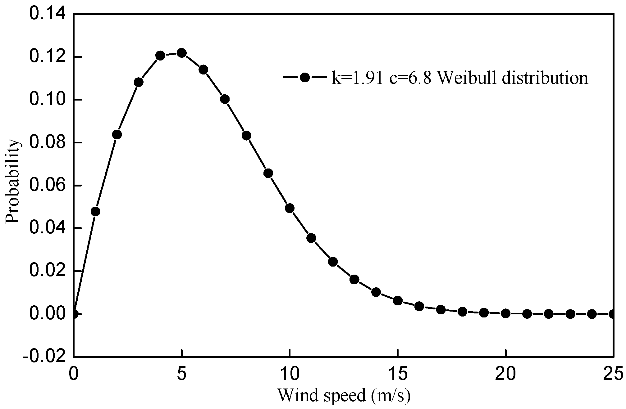
The basic parameters of the rotor, wind condition and NSGA-II algorithm are listed in
Table 4. The Weibull form factor and scaling factor are determined from local meteorological data of inland China with an annual average wind speed of 6 m/s, namely,
k = 1.91 and
A = 6.8 m/s. The probability distribution of the specified wind speed is shown in
Figure 12.
Table 4.
Parameters of rotor, wind condition and non-dominated sorting genetic algorithm (NSGA)-II algorithm.
Table 4.
Parameters of rotor, wind condition and non-dominated sorting genetic algorithm (NSGA)-II algorithm.
| Parameter | Value | Unit |
|---|
| Rotor diameter | 77 | m |
| Number of blades | 3 | - |
| Hub diameter | 3 | m |
| Hub height | 75 | m |
| Rated wind speed | 12 | m/s |
| Rated rotational speed | 19 | rpm |
| Rated power | 1500 | kW |
| Cut-in wind speed | 4 | m/s |
| Cut-out wind speed | 25 | m/s |
| Air density | 1.225 | kg/m3 |
| Weibull form factor k | 1.91 | - |
| Weibull scaling factor A | 6.8 | m/s |
| Number of individuals | 40 | - |
| Number of iterations | 30 | - |
| Probability of crossover | 0.8 | - |
| Probability of mutation | 0.05 | - |
Figure 12.
Weibull probability distribution of wind speed.
Figure 12.
Weibull probability distribution of wind speed.
Figure 13 shows the Pareto front obtained by taking the maximum AEP and the minimum blade mass as the optimization objectives. The points on the left hand of the front identify design solutions having low mass yet low energy production, whereas the points on the right hand of the front present design solutions having high energy production but also high mass, which indicates there are some conflicts between the two objectives. It cannot be said which point is the best, the choice of the solution in the practical design should be made according to the designer’s favor.
In order to explain the formation of the Pareto front better, four optimized schemes extracted at different positions on the Pareto front are analyzed, as marked in
Figure 13. The values of the design variables of schemes A, B, C, D and the original scheme are listed in
Table 5.
Figure 13.
Pareto front of two objectives.
Figure 13.
Pareto front of two objectives.
Table 5.
Values of the design variables.
Table 5.
Values of the design variables.
| Parameter | Original Scheme | Scheme A | Scheme B | Scheme C | Scheme D | Unit |
|---|
| x1 | 3.08 | 2.70 | 2.60 | 2.47 | 2.44 | m |
| x2 | 2.88 | 2.64 | 2.56 | 2.43 | 2.41 | m |
| x3 | 2.30 | 2.21 | 2.15 | 2.10 | 2.08 | m |
| x4 | 1.82 | 1.66 | 1.64 | 1.61 | 1.60 | m |
| x5 | 1.21 | 1.16 | 1.16 | 1.19 | 1.17 | m |
| x6 | 8.73 | 10.69 | 10.38 | 9.70 | 9.56 | ° |
| x7 | 6.64 | 6.72 | 6.61 | 6.59 | 6.60 | ° |
| x8 | 3.14 | 3.84 | 3.49 | 3.80 | 3.58 | ° |
| x9 | 0.43 | 0.85 | 0.82 | 0.88 | 0.97 | ° |
| x10 | −1.13 | −0.49 | −0.81 | −0.22 | 0.02 | ° |
| x11 | 6.75 | 7.73 | 6.96 | 7.10 | 7.03 | m |
| x12 | 9.50 | 9.81 | 9.32 | 10.51 | 9.73 | m |
| x13 | 14.10 | 14.18 | 14.32 | 14.34 | 14.21 | m |
| x14 | 28.95 | 24.32 | 25.16 | 24.35 | 24.20 | m |
| x15 | 19.0 | 15.5 | 15.6 | 15.2 | 14.9 | rpm |
| x16 | 33 | 32 | 30 | 30 | 29 | - |
| x17 | 43 | 38 | 36 | 35 | 34 | - |
| x18 | 53 | 48 | 46 | 44 | 44 | - |
| x19 | 62 | 53 | 51 | 50 | 48 | - |
| x20 | 53 | 41 | 39 | 38 | 38 | - |
| x21 | 43 | 33 | 31 | 30 | 30 | - |
| x22 | 33 | 29 | 29 | 29 | 28 | - |
| x23 | 7.8 | 7.6 | 8.0 | 7.6 | 7.8 | m |
| x24 | 11.0 | 12.1 | 11.8 | 11.9 | 11.8 | m |
| x25 | 18.0 | 17.9 | 17.9 | 17.7 | 17.7 | m |
| x26 | 21.4 | 21.3 | 21.3 | 21.3 | 21.2 | m |
| x27 | 0.188 | 0.195 | 0.180 | 0.193 | 0.191 | m |
| x28 | 0.620 | 0.589 | 0.558 | 0.553 | 0.551 | m |
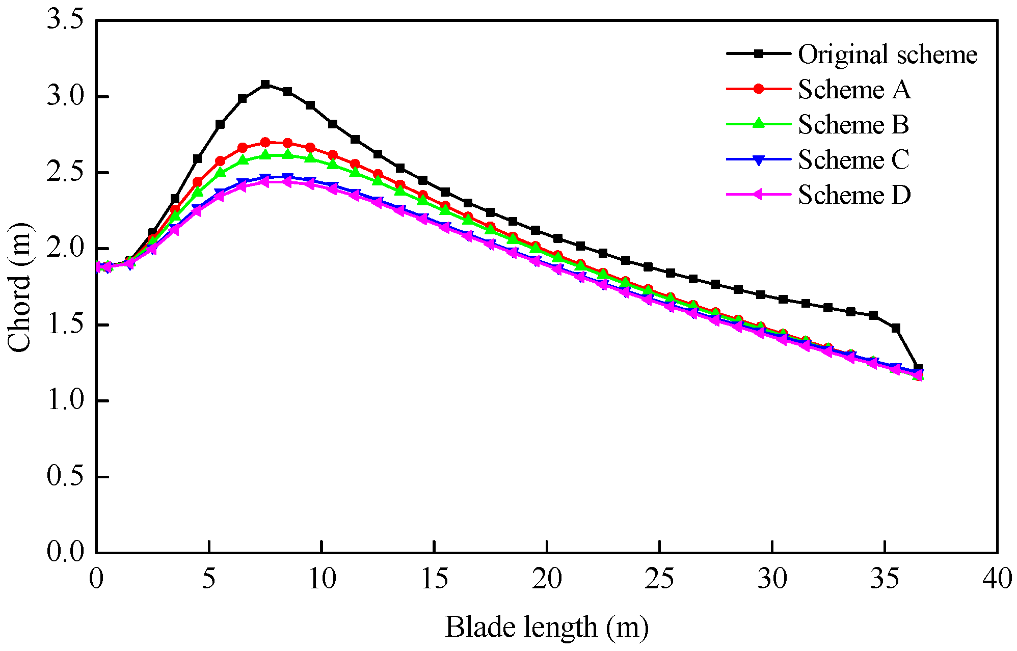
Figure 14 shows the chord distributions of the original scheme and optimized schemes. Due to the blade root diameter remaining the same, the chords of the optimization schemes change slightly in the root area. After the root area, the chords of the optimized schemes show an obvious decrease when compared to the original scheme, especially in the maximum chord region and near the blade tip. This indicates that the original scheme is possibly designed by the conventional methods (Wilson method or Glauert method), which leads to a larger chord. The reduction of the chord could reduce the power production to some extent, but it can result in a lighter blade and a lower thrust at the same time.
Figure 14.
Comparison of chord distribution.
Figure 14.
Comparison of chord distribution.
Figure 15 shows the twist distributions of the five schemes. The twists of the optimized schemes also change slightly in the root area for structural reasons. Then, the twists increase from the maximum chord region, but the distribution trends almost remain the same as the original scheme. Due to the decreasing of the rotational speed (
listed in
Table 5), the angle between the mean relative velocity and tangential direction will increase. With the incensement of the twist, the angle of attacks can almost remain the same, which guarantees the airfoils still have higher lift-to-drag ratios to partly make up for the power loss caused by the reduction of the chord.
Figure 15.
Comparison of twist distribution.
Figure 15.
Comparison of twist distribution.
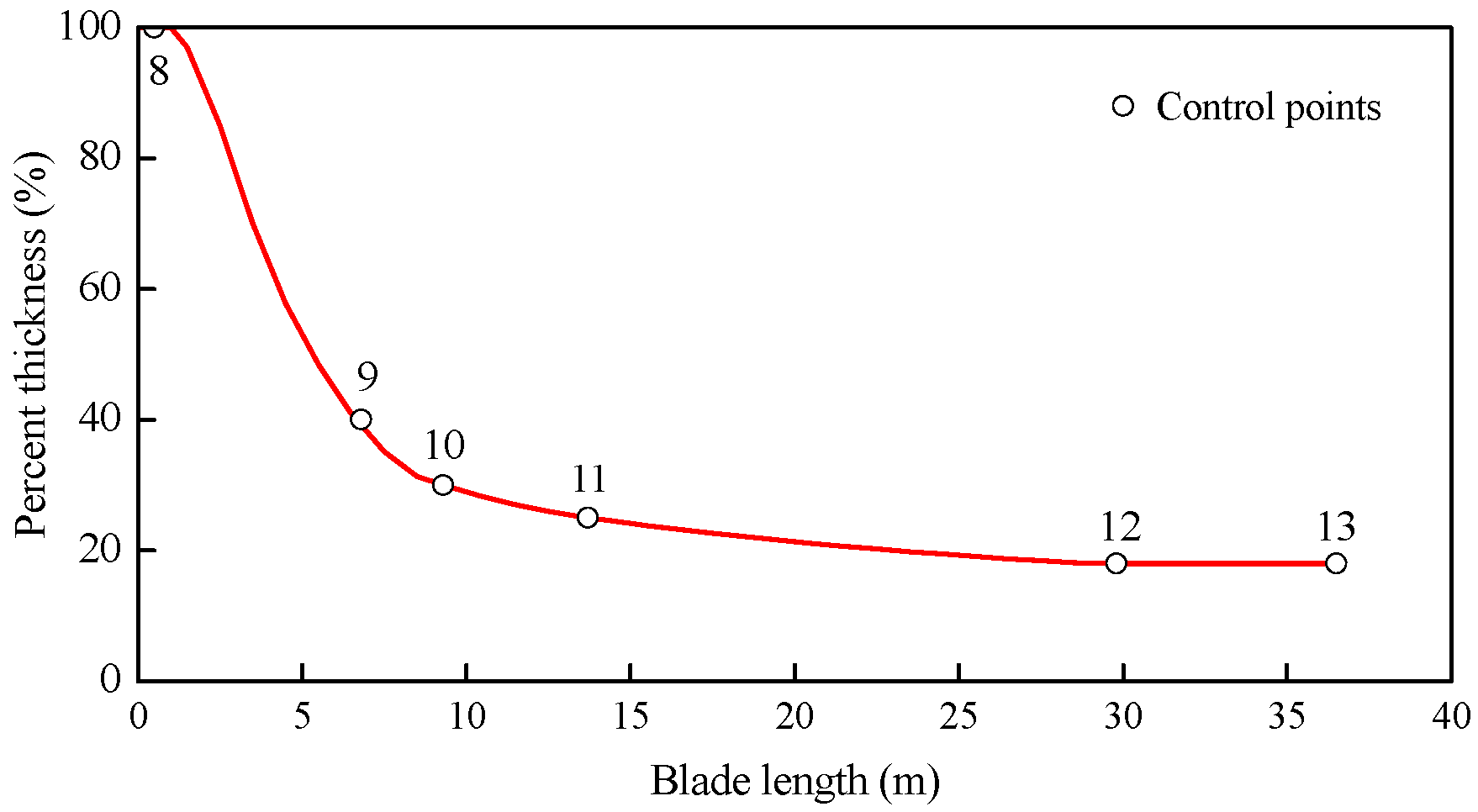
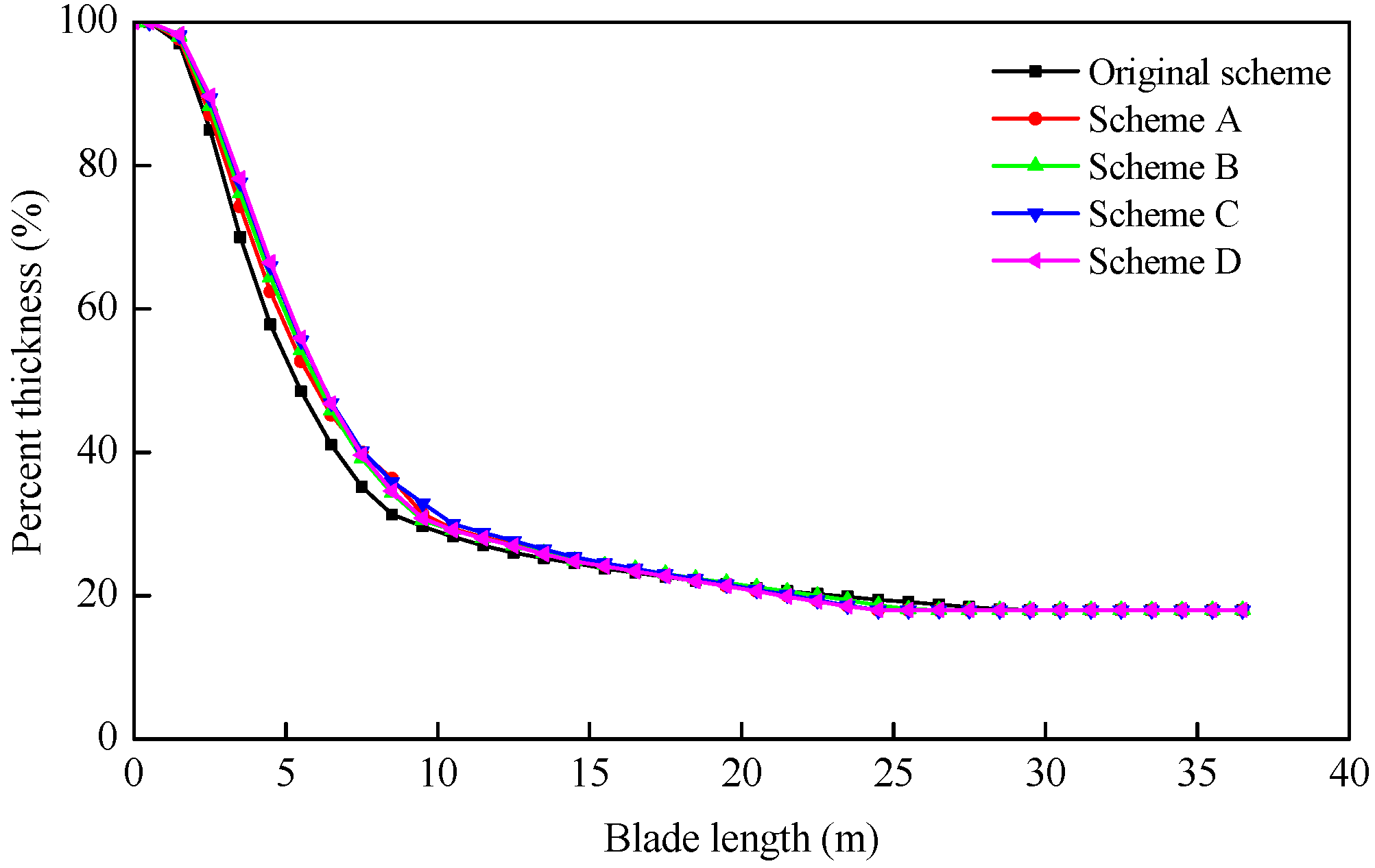
The percent thickness distributions are shown in
Figure 16. The locations of the airfoils with 40% and 30% thicknesses for the optimized schemes move toward the tip. From the structural point of view, this is good for increasing the section moment of inertia. The location of the airfoil with 25% thickness almost remains the same, while that of the airfoil with 18% thickness moves toward the root. As the airfoil with 18% thickness has a higher lift-to-drag ratio, the aerodynamic region composed by this airfoil is the main part of the blade to capture wind energy. Moving the location of the airfoil with 18% thickness towards the root can increase the length of this region, which is beneficial to capture more energy, thus improving the power efficiency from the aerodynamic point of view. The blade shapes become much smoother after optimization, which is more convenient for manufacturing. The decreasing of the rotational speed could reduce the rotor rotation times during a 20 year life span, and thus improve the fatigue life of the blade.
Figure 16.
Comparison of percent thickness distribution.
Figure 16.
Comparison of percent thickness distribution.
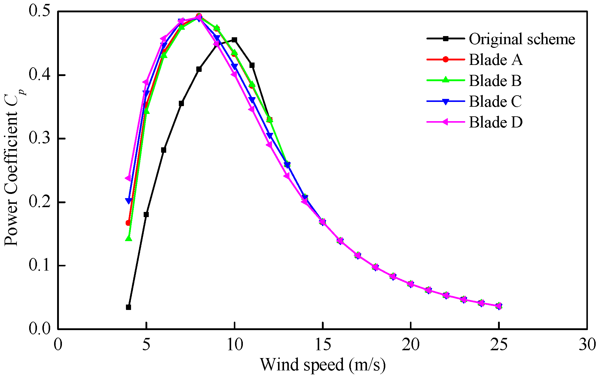
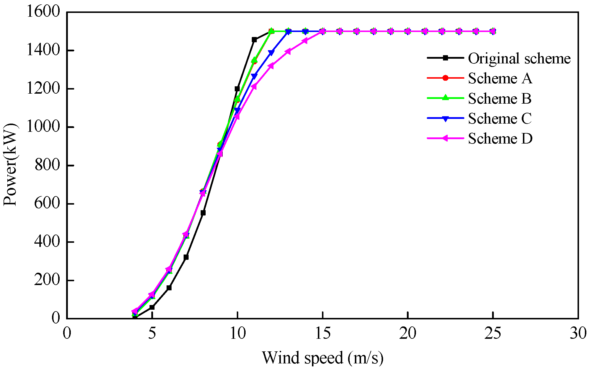
Figure 17 and
Figure 18 show the comparison of power coefficients and powers between the original scheme and optimized schemes, respectively. When compared to the original scheme, the power coefficients of the optimized schemes increase significantly in the speed range of 4 to 8 m/s, and decrease slightly in the peed range of 10 to 13 m/s. The power coefficients of the optimized schemes all reach the maximum values of about 0.49 at 8 m/s wind speed (a 7.7% increase compared to the original scheme), and keep relatively high values in the speed range of 6 to 9 m/s. With the reduction of chord, the rated wind speeds of the 4 optimized schemes gradually change from 12 to 15 m/s, as shown in
Figure 15. The comparisons in
Figure 17 and
Figure 18 reveal that the optimized schemes have better aerodynamic performances than the original scheme at low wind speeds, but the performances gradually become worse when the wind speed increases. As can be seen from
Figure 12, for a turbine site with an annual average wind speed of 6 m/s, the probabilities of the wind speed lying between 4 m/s and 8 m/s are much higher than those lying between 10 m/s and 13 m/s, so the optimized schemes are more reasonable as they can utilize more wind energy resources.
Figure 17.
Comparison of power coefficient under different wind speed.
Figure 17.
Comparison of power coefficient under different wind speed.
Figure 18.
Comparison of power under different wind speed.
Figure 18.
Comparison of power under different wind speed.
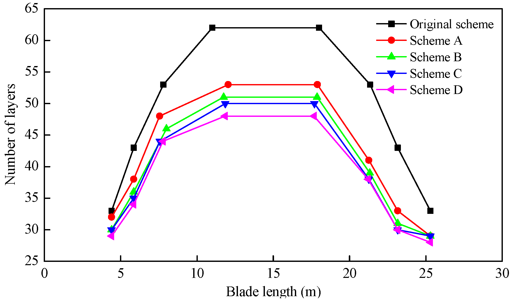
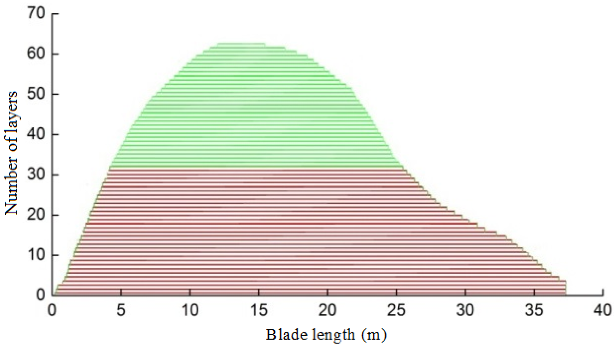
Figure 19 shows the comparison of material layup in the spar cap between the original scheme and optimized schemes. From
Figure 19 and
Table 4, it can be seen that the number of layers changes slightly from 4.4 m to 8 m and 21.5 m to 25.3 m while it decreases obviously from 8 m to 21.5 m along span-wise of the blade, and the thickest region becomes smaller. This indicates that the two regions from 4.4 m to 8 m and 21.5 m to 25.3 m have less impact on the blade mass than the middle part. The reason is that the original number of layers in these two regions is less, and the relatively large lower bounds limit it to change significantly. As the region from 4.4 m to 8 m withstands higher loads, the number of layers in this region is a bit more than it in the region from 21.5 m to 25.3 m after optimization.
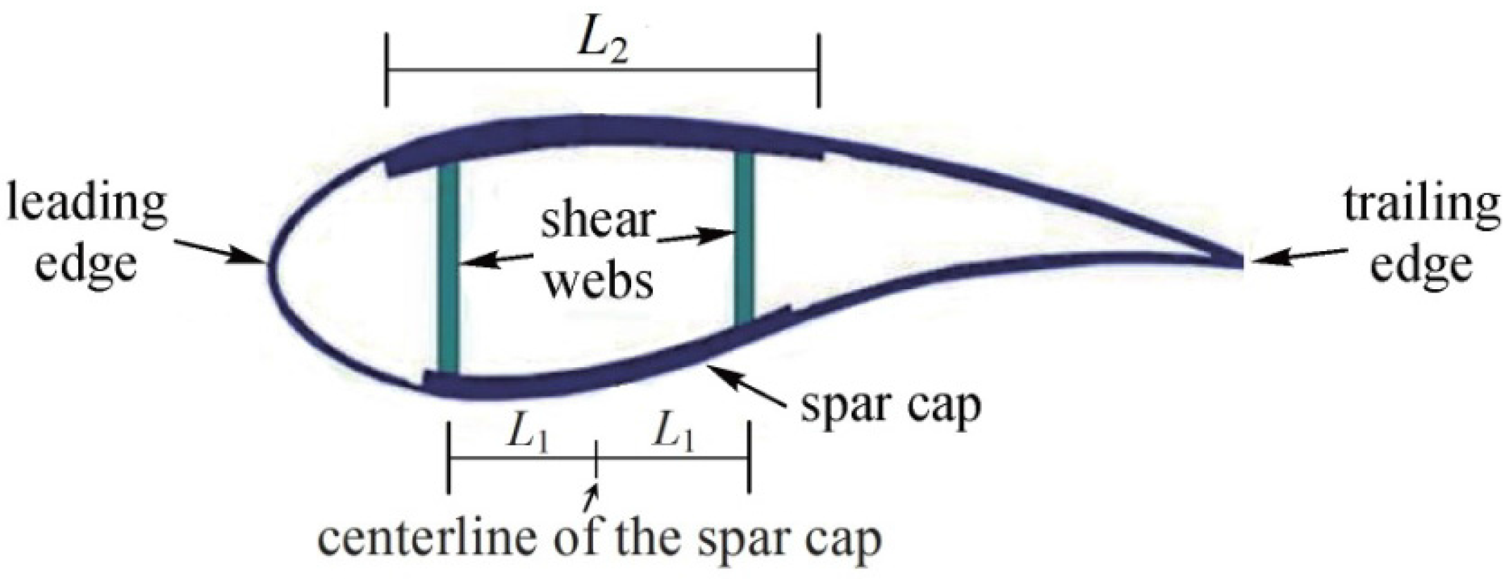
The position of the shear webs decrease after optimization, which means that the shear webs move toward the centerline of the spar cap. According to the sensitive analysis in our previous work [
29], although the blade mass will increase from 6555.2 kg to 6560.2 kg when the position was reduced by 20%, the maximum strain can reduce from 0.00429 to 0.00412,
i.e., improve the blade strength on the premise that the mass is almost unchanged. Thus, the number of layers in the spar cap could decrease further, which makes the blade much lighter. The width of the spar cap also decreases after optimization, and a smaller width of the spar cap can reduce the amount of materials, which is beneficial for reducing the blade mass.
Figure 19.
Comparison of material layup of the spar cap.
Figure 19.
Comparison of material layup of the spar cap.
The AEP, blade mass and structural performances of the schemes are presented in
Table 6. Compared with the original scheme, the AEP of schemes A, B, C, D increase by 11.40%, 10.99%, 9.48% and 7.56%, respectively, while the blade mass decreases by 10.39%, 13.53%, 15.33% and 15.96%, respectively. The maximum strain increases, the tip deflection decreases firstly and then increases, and the lowest buckling load factor decreases, but they still satisfy the constraint conditions set in the procedure. The structural stiffness reduces with the decreasing of the blade. However, the reduced ratio of the stiffness is greater than that of the mass of the blade. Therefore, the first natural frequency decreases, but there is no occurrence of resonance. Compared with the best result having a blade mass of 6064.6 kg in [
15], the reduction of chords and spar width can further decrease the blade mass obviously in the case of a small difference between the material layups.
Table 6.
Comparison of the annual energy production (AEP), blade mass and structural performance.
Table 6.
Comparison of the annual energy production (AEP), blade mass and structural performance.
| Scheme | AEP (GWh/Year) | Blade Mass (kg) | Maximum Strain | Maximum Tip Deflection (m) | The Lowest Buckling Eigenvalue | The First Natural Frequency (Hz) |
|---|
| Original | 3.175 | 6555.2 | 0.00429 | 4.60 | 2.024 | 1.027 |
| A | 3.537 | 5874.1 | 0.00481 | 4.13 | 1.491 | 0.969 |
| B | 3.524 | 5668.4 | 0.00485 | 4.36 | 1.358 | 0.938 |
| C | 3.476 | 5550.3 | 0.00491 | 4.75 | 1.252 | 0.907 |
| D | 3.415 | 5509.1 | 0.00498 | 4.92 | 1.216 | 0.884 |
6. Conclusions
This paper describes a multi-objective optimization method for the aerodynamic and structural integrated design of HAWT blades. The method is used to obtain the best trade-off solutions between the two conflict objectives of maximum AEP and minimum blade mass.
A procedure uses BEM theory and an FEM model, and the NSGA II algorithm is developed for this purpose. The BEM theory and FEM model are utilized to determine the aerodynamic and structural performances of HAWT blades, and the optimization fitness functions as well. The NSGA II algorithm is adopted to handle the design variables chosen for optimization and search for the group of optimal solutions following the basic principles of Genetic Programming and Pareto concepts.
The procedure has been applied successfully to a 1.5 MW commercial HAWT blade, and satisfactory schemes to increase the AEP and decrease the blade mass are achieved under a specific annual average wind speed. The results indicate that the maximum AEP requires blades having large chords and layer thicknesses, thus high masses, while the requirement of the maximum blade mass is just the opposite. The further aerodynamic and structural analysis of the optimization schemes show great improvements for the overall performances of the blade, which indicates the efficiency and reliability of the proposed procedure.
In future work, an attempt will be made to define the chord and the twist distributions more appropriately with Non-Uniform Rational B-Splines (NURBs) curves. The optimization of the material layup in the whole spar cap will also be carried out to further improve the overall performances of the blade.


