Ensemble Learning Approach for Probabilistic Forecasting of Solar Power Generation

Abstract

Probabilistic forecasting accounts for the uncertainty in prediction that arises from inaccurate input data due to measurement errors, as well as the inherent inaccuracy of a prediction model. Because of the variable nature of renewable power generation depending on weather conditions, probabilistic forecasting is well suited to it. For a grid-tied solar farm, it is increasingly important to forecast the solar power generation several hours ahead. In this study, we propose three different methods for ensemble probabilistic forecasting, derived from seven individual machine learning models, to generate 24-h ahead solar power forecasts. We have shown that while all of the individual machine learning models are more accurate than the traditional benchmark models, like autoregressive integrated moving average (ARIMA), the ensemble models offer even more accurate results than any individual machine learning model alone does. Furthermore, it is observed that running separate models on the data belonging to the same hour of the day vastly improves the accuracy of the results. Getting more accurate forecasts will help the stakeholders come up with better decisions in resource planning and control when large-scale solar farms are integrated into the power grid.

1. Introduction

Fossil fuels have been the most widely-used energy sources for centuries and continue to be so. Unfortunately, both the production and utilization of fossil fuels results in the release of green house gases in the atmosphere. This environmental impact has been even more aggravated in recent years as we try to extract less accessible resources, which results in higher emission of green house gases with the need for additional transportation of those resources [1]. Between 2010 and 2040, the world is going to see a rise in energy demand by 56% [2]. With this ever-increasing energy demand and with its associated pollution, the world is looking for renewable energy sources. Renewable energy and nuclear power are the fastest growing alternative energy resources, growing at the rate of 2.5 percent every year [2]. Alternative energy sources are important as they can reduce the need to export/import energy and also stabilize price fluctuations in the energy market.

In recent years, solar energy has gained much importance because of the advances in photovoltaic (PV) technology and also its environmental friendliness. Solar PV power plants do not emit any green house gases and use no or very little water resources. Solar energy is also the most abundant resource naturally available, with one hour of solar energy striking the Earth sufficient for the energy needs of the world’s entire population for a year [3]. The technology road map for solar PV estimates 4600 GW of PV capacity by 2050, and that will result in the reduction of four gigatonnes (Gt) of carbon dioxide per year [4].

The integration of large solar farms into the power grid is not an easy task, as the output of solar farms varies with every season. It also depends on various other factors, like cloud cover, wind speed, humidity, etc. One critical phenomenon to consider is the ramp event, which occurs when the solar power generation suddenly drops when there is cloud cover and ramps up again when the cloud cover lifts [5]. With all of these factors in consideration, solar power forecasting comes to play an important role. Forecasting the solar power several hours ahead could facilitate balancing the grid’s supply and demand by helping the stakeholders make informed decisions regarding backup power generation using fossil fuel, demand response, peak load shifting, etc.

Our Contributions

In this study, we propose a method that uses an “ensemble” of multiple point (also known as single-valued) forecasts to generate probabilistic forecasts 24 h ahead. We use the 12 variables obtained from 24-h ahead numerical weather prediction (NWP) by the European Centre for Medium-Range Weather Forecasts (ECMWF) as the input attributes to our ensemble method.

Firstly, we group the data based on their zones and hours of the day. Secondly, we deploy seven machine learning-based regression models (namely: (1) Decision tree; (2) Gradient boosting; (3) K-nearest neighbors (KNN) with uniform weights; (4) KNN with distance-based weights; (5) Lasso; (6) Random forests; and (7) ridge). All of these methods individually outperform the three benchmark models, like ARIMA, which are widely used in time series forecasting.

Then, the point forecasting outputs from those seven regression models are combined to generate probabilistic forecasting using three different ensemble methods (namely: (1) Linear; (2) Normal distribution; and (3) normal distribution with additional features), all of which give better results than any of those seven models can offer individually. In addition, we have demonstrated that grouping of the data by the hour of the day vastly improves the accuracy of the forecasting results.

Our proposed method is district from the existing probabilistic solar forecasting methods like [6,7] because we use literally different base regression models rather than using a single base model with different parameters or bootstrapping. The good results offered by it can be attributed to the soundness of the seven base regression models themselves and the effectiveness of our carefully-crafted ensemble strategies, especially in the case of the normal distribution with additional features method.

A preliminary version of this study has been presented as [8]. In this current paper, we have significantly extended our work by incorporating a more detailed description of our proposed method, as well as much more comprehensive experimental results. It is a summary version of the master’s thesis [9] written by the first author and advised by the second author.

The remainder of the paper is organized as follows. Section 2 presents the related pieces of work. Section 3 describes the solar power forecasting dataset that we use, as well as the problem formulation. Section 4 describes the proposed methods to generate the probabilistic forecasts. Section 5 details our experimental setup. Section 6 presents the experiment results, and finally, conclusions are drawn in Section 7.

2. Related Work

2.1. Point Forecasting

In the domain of solar forecasting, point forecasting methods, which yield only a single forecasted value for each forecasting instance, have been widely used. Point forecasting methods can be subdivided into two broad categories: statistical and machine learning methods. Some instances of those two categories for solar forecasting are presented in the following Section 2.1.1 and Section 2.1.2, respectively.

2.1.1. Statistical Methods

Bacher et al. [10] introduced a two-stage model for online short-term solar power forecasting. In the first stage, the clear sky model is used to normalize the solar power, and in the second stage, linear time series models are used to forecast the solar power.

Y. Huang et al. [11] provided a comparative analysis of physical and statistical forecasting models for PV stations. In the physical forecasting model, a physical modeling of the PV panels is carried out to obtain the forecast, whereas in the statistical model, the past power values are used as an input to predict the future values.

J. Huang et al. [12] described a method to forecast one-hour ahead solar radiation during cloudy days. It combined an autoregressive model with a dynamical system model. In addition, the difference of solar radiation values at the present and lag one time step was used as a correction to a predicted value, improving the forecasting accuracy by up to 30%.

2.1.2. Machine Learning Methods

In Marquez et al. [13], the authors used an artificial neural network (ANN) model to forecast the global and the direct solar irradiance with the help of the National Weather Service’s (NWS) database. Eleven input variables are used in total: nine meteorological variable from the NWS database and two additional variables of solar zenith angle and normalized hour angle.

Hossain et al. [14] proposed a hybrid intelligent predictor for 6-h ahead solar power prediction. The system used an ensemble method with 10 widely-used regression models, namely, linear regression (LR), radial basis function (RBF), support vector machines (SVM), multi-layer perceptron (MLP), pace regression (PR), simple linear regression (SLR), least median square (LMS), additive regression (AR), locally-weighted learning (LWL) and IBk (an implementation of the k-nearest neighbor algorithm).

Zhu et al. [15] decomposed the output power of the PV plant using wavelet decomposition to separate useful information from disturbances. Then, ANNs are used to build the models of the decomposed PV output power. Finally, the outputs of the ANN models are reconstructed into the forecasted power of the PV plant.

In [16], Li et al. used a hierarchical forecasting approach to evaluate and compare the two common methods, ANN and support vector regression (SVR), for predicting energy productions from a solar photovoltaic system in Florida, USA, 15 min, 1 h and 24 h ahead of time, respectively.

Diagne et al. [17] and Antonanzas et al. [18] are the two recent comprehensive survey papers on solar power/irradiance forecasting methods, where most of them are the point forecasting ones.

2.2. Probabilistic Forecasting

Every forecast carries with it a certain amount of uncertainty because of the errors in real-time measurements and the uncertainty of the prediction models themselves. No forecast is perfect. “Probabilistic forecasting” [19] is the forecast that assigns a probability to each of a number of different future events. Probabilistic forecasts are preferred to point forecasts (also known as single-valued forecasts) as they take into account the uncertainties in the predicted values, which helps in assessing the risk when a decision is made. Probabilistic forecasts are being used widely in the case of predicting binary events, e.g., events like “what is the probability that it rains today?” and other similar events. However, now, the focus is shifting towards applying them to more general events, like flood risk assessment, weather prediction and financial risk management, to name a few [19].

Probabilistic forecasting has been stated to be have been explored in solar forecasting in recent years. Iversen et al. [6] proposed a framework for calculating the probabilistic forecasts of solar irradiance using stochastic differential equations (SDE). They construct a process that is limited to a bounded state space, and it assigns zero probability to all of the events outside this state space.

More recently, Grantham et al. [7] also proposed a probabilistic forecasting method for solar radiance. They presented a new data-driven approach for constructing a full predictive density of solar radiance based on a nonparametric bootstrap. They demonstrated the usefulness of the new bootstrapped statistical ensembles for probabilistic one-hour ahead forecasting in Mildura, Australia.

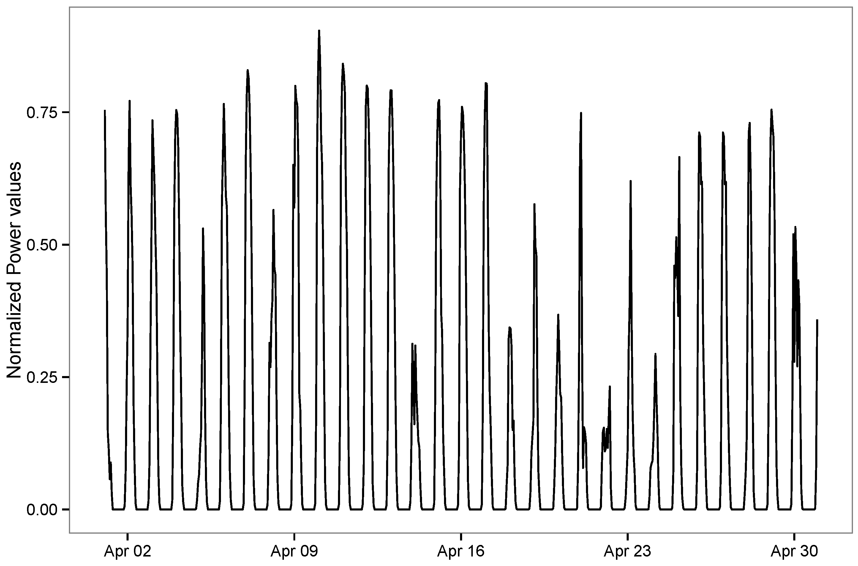
3. Dataset and Problem Formulation

The data used in this study are provided by the organizers of the Global Energy Forecasting Competition (GEFCOM) 2014 [20,21,22]. The initial training dataset consists of 12 months of hourly solar power data from April 2012 to March 2013. The testing dataset consists of 15 months of data from April 2014 to June 2015. After the forecasting has been done for each month in the testing dataset, that month’s data are incrementally added into the training dataset.

The data are collected from three solar farms (denoted as zones) which are adjacent to each other in a certain region of Australia, with the following installation parameters (the exact locations of the farms are not disclosed by the GEFCOM organizers):

• Zone 1: altitude = 595 m; panel type = Solarfun SF160-24-1M195; No. of panels = 8; nominal power = 1560 W; panel orientation = 38°clockwise from north; panel tilt = 36°.
• Zone 2: altitude = 602 m; panel type = Suntech STP190S-24/Ad+; No. of panels = 26; nominal power = 4940 W; panel orientation = 327°clockwise from north; panel tilt = 35°.
• Zone 3: altitude = 951 m; panel type = Suntech STP200-18/ud; No. of panels = 20; nominal power = 4000 W; panel orientation = 31°clockwise from north; panel tilt = 21°.

The data consist of the hourly measurements of 12 input variables (also known as attributes or features) that affect the solar power generation. They are generated 24 h (one day) ahead [21] by the European Centre for Medium-Range Weather Forecasts (ECMWF) [23] using numerical weather prediction (NWP) [24]. These 12 input variables are listed below.

• tclw: Total column liquid water, vertical integral of cloud liquid water content. Unit of measurement: kg/m².
• tciw: Total column ice water, vertical integral of cloud ice water content. Unit: kg/m².
• SP: Surface pressure. Unit: Pa.
• r: Relative humidity at 1000 mbar, defined with respect to saturation over ice below −23 °C and over water above 0 °C. For the period in between, a quadratic interpolation is applied. Unit: %.
• TCC: Total cloud cover. Unit: zero to one.
• 10u: 10-meter Uwind component. Unit: m/s.
• 10v: 10-meter Vwind component. Unit: m/s.
• 2T: two-meter temperature. Unit: K.
• SSRD: Surface solar radiation down. Unit: J/m².
• STRD: Surface thermal radiation down. Unit: J/m².
• TSR: Top net solar radiation, net solar radiation at the top of the atmosphere. Unit: J/m².
• TP: Sum of convective precipitation and stratiform precipitation. Unit: m.

The output variable is the solar power generated in each farm at each hour. This value is normalized to lie between zero and one as the nominal power generated in each of the solar farms is different.

The solar power forecasting problem we are trying to solve can be formulated as follows. Suppose we are currently at hour h (where $h\in \{0,\dots ,23\}$) of day d. Our aim is to forecast the solar power output of zone z (where $z\in \{1,2,3\}$) at hour h of day $d+1$ by using the 12 input variables, which are the 24-h ahead forecasted weather measurements by ECMWF for hour h of day $d+1$ for the geographical area in which zone z is located. As such, the forecasting problem we are trying to solve is a supervised learning one rather than a univariate time series forecasting.

4. Proposed Method

Our proposed method uses an “ensemble” of different machine learning algorithms to generate the probabilistic forecasts. In [25], Bell and Koren presented the first-prize winning method in the $1 million Netflix prize challenge and observed that an ensemble approach using different predictors offered the best results. The reason behind this phenomenon is that each machine learning algorithm performs well only with specific type(s) of data. For example, SVM and ANN perform better with multi-dimensional data and continuous features. On the other hand, decision tree and rule-based learners perform well with categorical data. Likewise, SVM and ANN models perform at their best when dealing with large sample sizes, whereas naive Bayes models require only a small sample size [26]. Thus, in order to take advantage of the strengths of various algorithms in various situations, ensemble methods are employed.

In this work, we follow an ensemble regression strategy for forecasting. First, we group the data based on zones and hours of the day. Then, we generate the point forecasts using seven individual machine learning-based regression models. Finally, we combine those point forecasts into the probabilistic forecasts using three different ensemble methods.

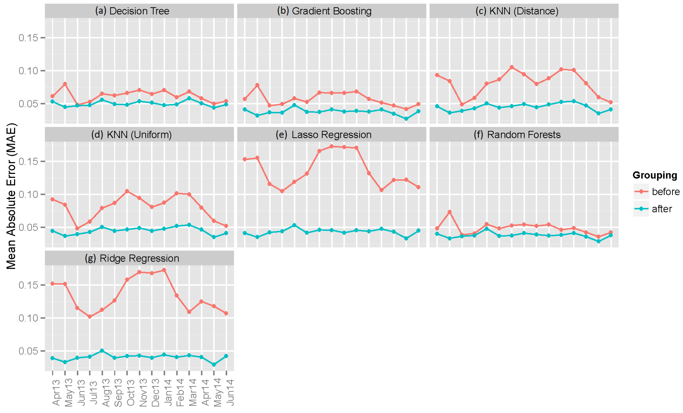
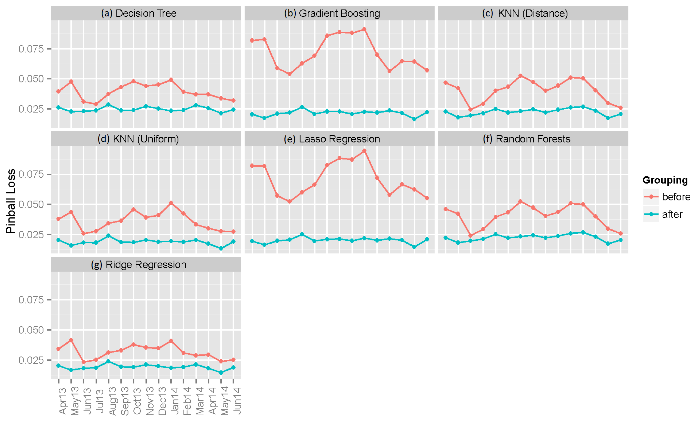
4.1. Grouping of Data

As mentioned above in Section 3, the data consist of those from 3 different solar farms (zones), and the power generated at each zone differs in magnitude. To avoid large fluctuations in the output values, the data are grouped based on zones. The solar power generated varies throughout the day, going to zero during the night. Hence, within each zone, the data are further grouped by each hour of the day. This gives us 24 different sets of data in each of the 3 zones (i.e., 24 × 3 = 72 datasets in total).

Figure 1 shows the values for the month of April 2012 in Zone 1. We can see that the values oscillate between 0 and 1 consistently throughout the month.

The dataset contains 12 input variables. Let X be a $(72t\times 13)$ matrix, where the 13th column is the output variable, i.e., solar power generated. Matrix X contains the data from the three different solar farms, Zones 1, 2 and 3, and t is the number of days in the training dataset.

Initially, the data are grouped based on the zone. Let $X_z$ denote the data from each zone where $z\in \{1,2,3\}$. $X_z$ is a $(24t\times 13)$ matrix. $X_z$ in turn contains the data for each of the 24 h in a day. Grouping $X_z$ based on each hour would give us the matrix $X_{zh}$, where z represents the zone and h represents the hour. $X_{zh}$ is a $(t\times 13)$ matrix.

At the end of the grouping process, we have 24 different datasets in each of the three zones, which results in 72 datasets in total. Hence, when we say, for instance, that the decision tree regressor is used to generate the point forecast, it means that 72 decision tree sub-models are built from 72 different datasets, and among them, a particular sub-model corresponding to the test instance at hand is selected to perform the point forecasting. For example, if we are to point forecast the solar power generated in Zone 1 at Hour 5 for a particular day, among the 72 different decision tree sub-models, we select the one built only from the historical data recorded at Hour 5 in Zone 1 in the training dataset.

For each sub-model dedicated to zone z and hour h, for the training phase, the input is a matrix $X_{zh}$ of size $(t\times 13)$, where t is the number of days in the training dataset, and the output is a regression model. For the testing (forecasting) phase, the input is a matrix $F_{zh}$ of size $(d\times 13)$ with its 13th column withheld, and the output is a matrix P of size $(d\times 1)$, where d is the number of days the forecasting is to be made. The training and testing processes are to be repeated 72 times to cover all of the combinations of zones and hours.

4.2. Generating Point Forecasts

After the data are grouped, the following machine learning-based regression models are used to generate the point forecasts. These algorithms are implemented using the Python scikit learn module [27]. The tunable parameters for each model are selected by a ten-fold cross-validation on the initial training dataset.

• Decision tree regressor: A model is fitted using each of the input variables. For each of the individual variables, the mean squared error is used to determine the best split. The maximum number of features to be considered at each split is set to the total number of features [28].
• Gradient boosting: An ensemble model that uses decision trees as weak learners and builds the model in a stage-wise manner by optimizing the loss function [29].
• KNN regressor (uniform): The output is predicted using the values from the k-nearest neighbors (KNNs) [30]. In the uniform model, all of the neighbors are given an equal weight. Five nearest neighbors are used in this model, i.e., $k=5$. The “Minkowski” distance metric is used in finding the neighbors.
• KNN regressor (distance): In this variant of KNN, the neighbors closer to the target are given higher weights. The choice of k and the distance metric are the same as above.
• Lasso regression: A variation of linear regression that uses the shrinkage and selection method. The sum of squares error is minimized, but with a constraint on the absolute value of the coefficients [31].
• Random forest regressor: An ensemble approach that works on the principle that a group of weak learners when combined would give a strong learner. The weak learners used in random forest are decision trees. Breiman’s bagger, in which at each split all of the variables are taken into consideration, is used [32].
• Ridge regression: It penalizes the use of a large number of dimensions in the dataset using linear least squares to minimize the error [33].

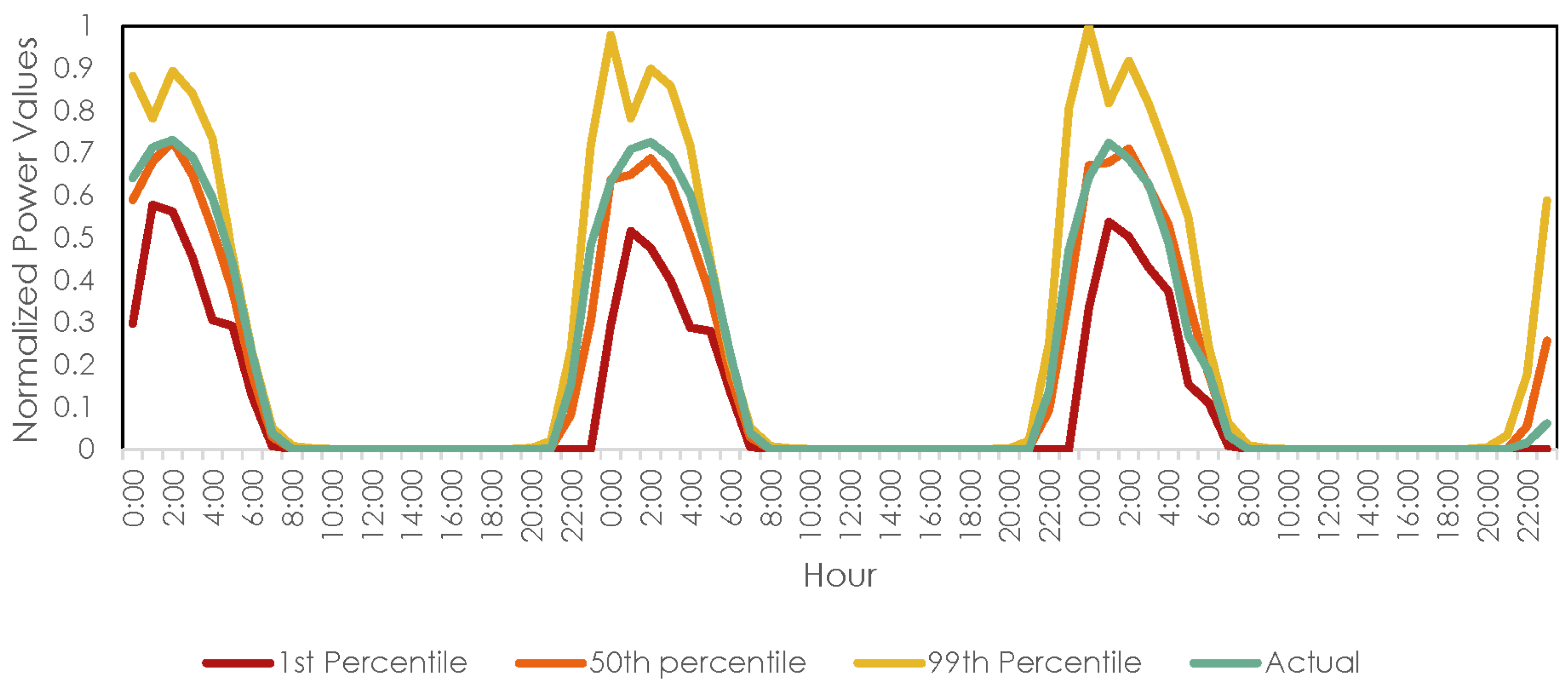
4.3. Generating Probabilistic Forecasts

We propose three different ensemble methods to generate the probabilistic forecasts using the point forecasts from the 7 machine learning models mentioned above.

4.3.1. Method I: Linear Method

The linear method is used to generate the 99 percentiles where the first percentile is the lowest among the point forecasts and the 99th percentile is the highest. The i-th percentile of a distribution is a number such that approximately i percent of the values in the distribution are equal or less than that number. For example, if we say that 12 is the 80th percentile of a distribution, then that means approximately 80% of the numbers in that distribution are less than or equal to 12.

Let $x_1,x_2,\dots ,x_n$ be a set of values where n represents the total number of observations, which are point forecasts in our case. Here, $n=7$ because we use 7 individual machine learning models to generate 7 distinct point forecasts. Following is the linear interpolation method, adapted from [34], to calculate the percentiles. First, we sort the data such that $x_1$ is the smallest value and $x_n$ is the largest. Then, we calculate the relative index of the i-th percentile, denoted as $r_i$, for $i=1,\dots ,99$ using Equation (1).

$$r_i=\frac{n·i}{100}+0.5$$

(1)

If $r_i$ is an integer, then $x_{r_i}$ will be the i-th percentile value. If $r_i$ is not an integer, then we can separate it into the integer part k and the fractional part f, respectively. Then, $p_i$, the interpolated i-th percentile value is calculated using Equation (2). We regard $x_0=x_1$ and $x_{n+1}=x_n$, respectively.

$$p_i=\left\{\begin{array}{cc}{x}_{r_i}\hfill & \mathrm{if}{r}_i\mathrm{is}\mathrm{an}\mathrm{integer}\hfill \\ (1-f)·x_k+f·x_{k+1}\hfill & \mathrm{otherwise}\hfill \end{array}\right.$$

(2)

4.3.2. Method II: Normal Distribution Method

Let the n point forecasts generated using n regression models be represented as $x_1,x_2,\dots ,x_n$ with a mean μ and standard deviation σ (note: $n=7$ in our case). For $i=1,\dots ,99$, finding the i-th percentile value $p_i$ is the same as finding $p_i$ such that $P(X<p_i)=i/100$. For that, we find the corresponding Z value, denoted as $z_i$, using the Z table or standard normal table [35] by looking for the table entry that is closest to $i/100$. Once we have the values of μ, σ and $z_i$, that of $p_i$ can be calculated using Equation (3).

$$p_i=\mu +z_i·\sigma$$

(3)

4.3.3. Method III: Normal Distribution Method with Additional Features

This method is similar to Method II, but now, we add two additional sets of regression models along with the original model set. In the first additional model set, we use an additional feature “month” of the year along with the existing 12 features. In the second additional model set, only the most recent 30 days of data (instead of the whole of the available training data) are considered to carry out the forecasts. All 7 individual machine learning regression models are deployed for both additional model sets. This results in $n=21$ regression models in total (7 for the original model set + 7 for the first additional model set + 7 for the second additional model set). Having more data points ($n=21$) helps smoothen the percentile curve when compared to those curves in Methods I and II, where fewer data points are available ($n=7$).

5. Experimental Setup

In this section, we will discuss the experimental setup that we use to evaluate the accuracy performance of our proposed methods described above in Section 4.

5.1. Training and Testing Datasets

As mentioned above in Section 3, we use data from the Global Energy Forecasting Competition (GEFCOM) 2014 [20,21,22] comprising 3 solar farms (zones). Each instance (record) corresponds to the hourly data with 12 input variables, which are the environmental variables, and 1 output variable, which is the generated solar power.

The initial training dataset consists of 12 months of hourly solar power data from April 2012 to March 2013. This corresponds to 365 days × 24 hours × 3 zones = 26,280 training instances.

The testing dataset consists of 15 month of data from April 2013 to June 2014. This corresponds to 456 days × 24 h × 3 zones = 32,832 test instances. Testing (forecasting) is carried out in a “monthly” fashion in 15 batches. For example, in the first testing month of April 2013, the forecasting for the 2160 test instances (i.e., 30 days × 24 h × 3 zones) is performed.

After the forecasting has been done for each month in the testing dataset, that month’s data are accumulated into the training dataset before forecasting is performed on the next month. For example, after the forecasting for April 2013 is done, its 2160 test instances (along with their actual observed values for the solar power output) are added to the training dataset, increasing its sizes to 26,280 + 2160 = 28,440 instances.

5.2. Evaluation Metrics

Three different metrics are used to evaluate our results.

Root mean square error (RMSE) and mean absolute error (MAE), the two most common metrics in regression analysis, are used to evaluate the point forecasts.

$$\mathrm{RMSE}=\sqrt{\frac{1}{N}\sum _{i=1}^N{(y_i-{\widehat{y}}_i)}^2}$$

(4)

$$\mathrm{MAE}=\frac{1}{N}\sum _{i=1}^N|y_i-{\widehat{y}}_i|$$

(5)

where N is the number of observations, $y_i$ is the observed value and ${\widehat{y}}_i$ is the forecasted value for $i=1,\dots ,N$. Lower values indicate better forecasts for both RMSE and MAE.

When it comes to probabilistic forecasts, RMSE and MAE cannot be used because we generate 99 percentile values for each forecast. Therefore, instead, we use the pinball loss function [36], which is a commonly-used error evaluation metric for probabilistic forecasts. Let the 99 percentile values (generated using either Equation (2) or Equation (3)) be defined as $p_1,p_2,\dots ,p_{99}$, respectively, $p_0=-\infty$ the natural lower bound and $p_{100}=+\infty$ the natural upper bound. Then, the pinball loss score for the i-th percentile $p_i(1\le i\le 99)$ with regard to the observed value y can be calculated as follows:

$$\text{pinball-loss}(p_i,y)=\left\{\begin{array}{cc}(1-i/100)(p_i-y)\hfill & \mathrm{if}y<p_i\hfill \\ (i/100)(y-p_i)\hfill & \mathrm{otherwise}\hfill \end{array}\right.$$

(6)

To evaluate the overall performance, this score is averaged across all of the target percentiles. Lower scores indicate better forecasts.

For point forecasts, we mimic the probabilistic forecasts by generating 99 percentiles all assuming the same forecasted values (note: the same approach was also used for the benchmark point forecasting method in the GEFCOM 2014 competition [22]).

5.3. Benchmark Models

In order to conduct a comparative performance analysis on the 7 individual machine learning models, as well as the 3 proposed ensemble models, we choose 3 commonly-used methods in the area of time series forecasting to serve as our benchmark models (note: since they are univariate time series models, only the solar power output time series itself is used as the input, but not ECMWF’s 12 forecasted weather measurements). The forecast package [37] in R [38] is used to implement these models. Their brief descriptions are as follows:

• ARIMA: The autoregressive integrated moving average (ARIMA) model is one of the most widely-used techniques in time series forecasting. The function auto.arima() from the forecast package [37] in R is used. It automatically detects the best parameters to fit the data.
• Naive: In this method, all of the forecasts are set to the last observed value. Surprisingly enough, this model works well for many economic and financial time series problems [39].
• Seasonal naive: This method is similar to the naive method, but the forecasts are set to the last observed value from the same season [39].

6. Experimental Results

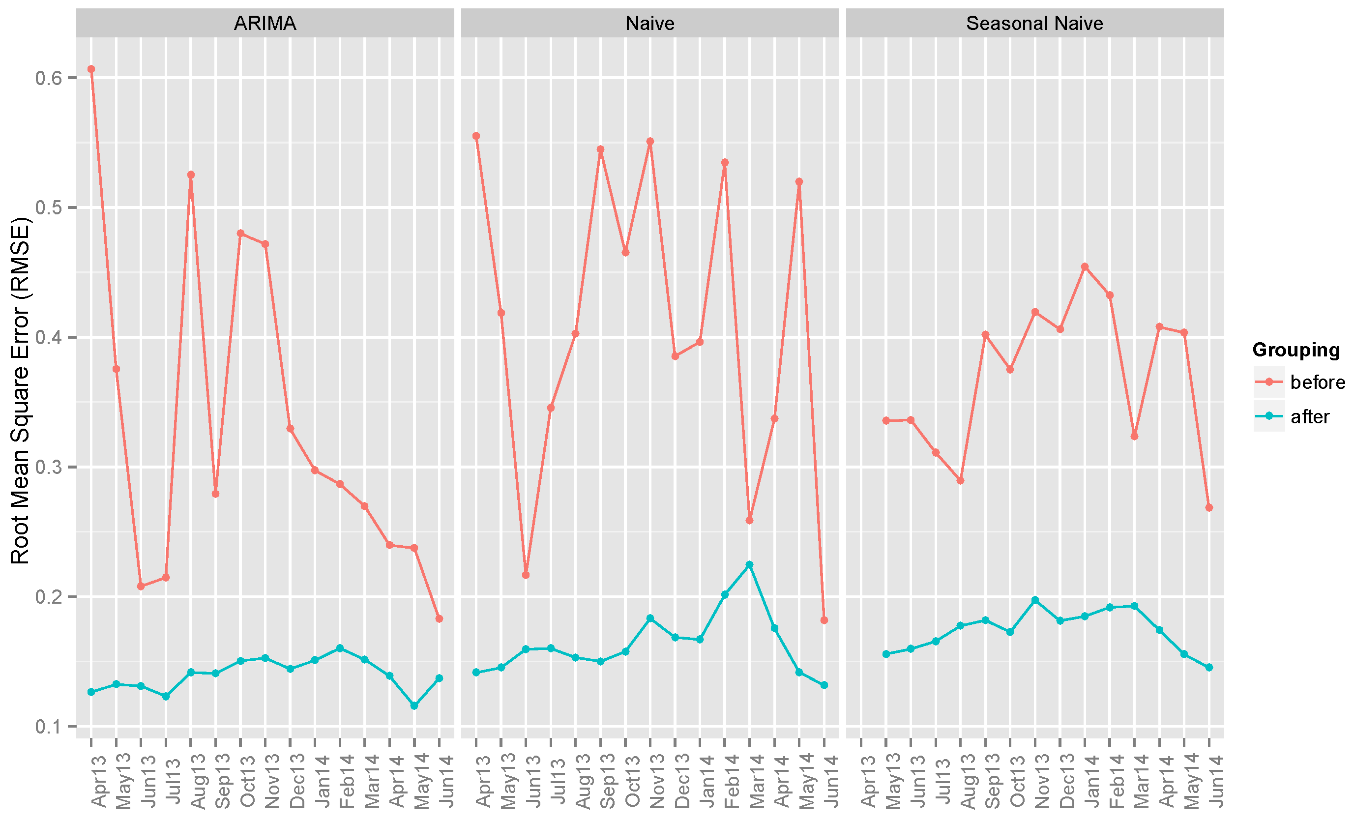
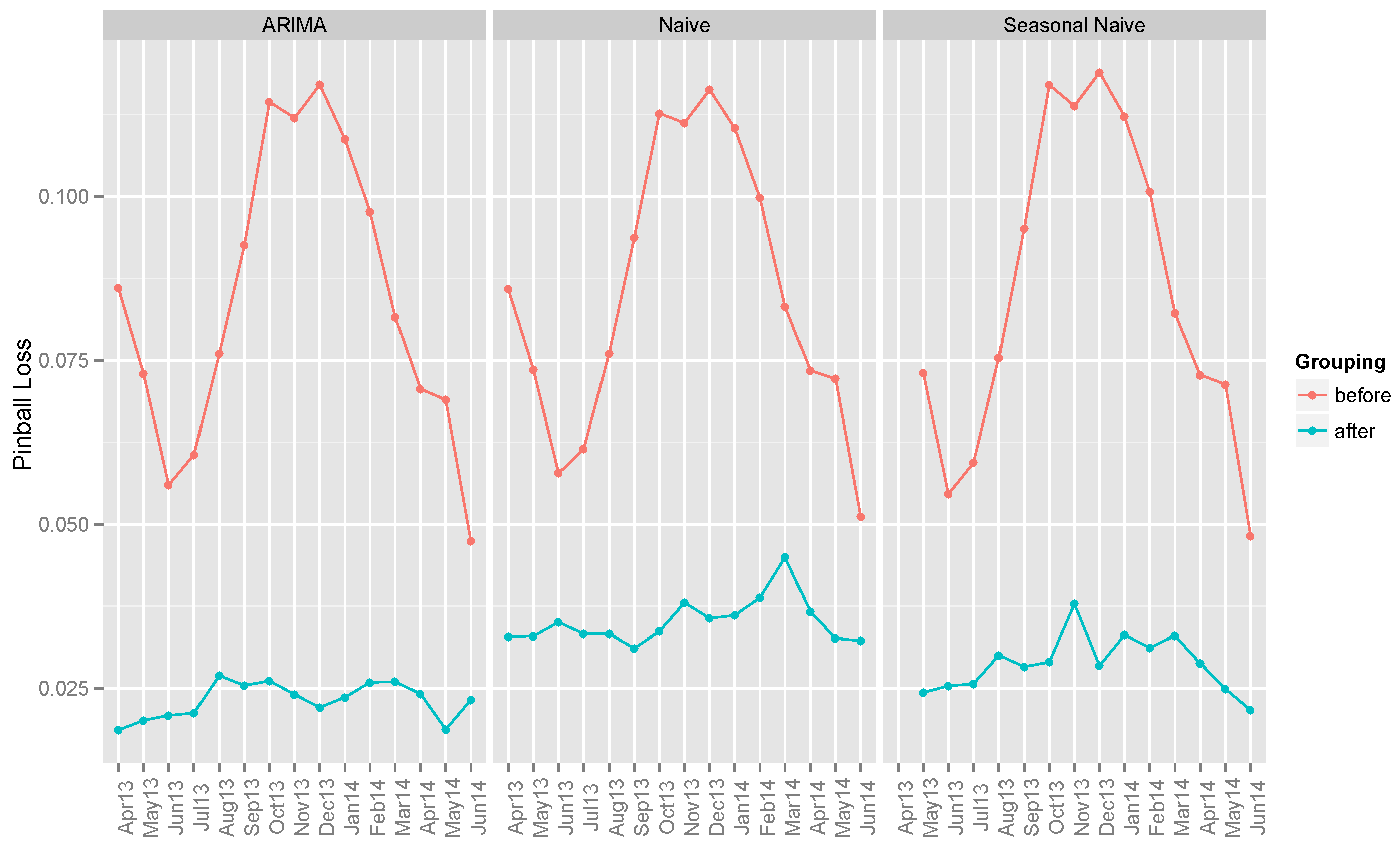
6.1. Benchmark Models

Figure 2 and Figure 3 show the RMSE and MAE values respectively of the three benchmark models. The results are the average RMSE/MAE values for each of the 15 months in the testing dataset across the three zones throughout the full 24-h period (including the night hours where the solar power output is zero).

Among the three models, ARIMA performs the best both in terms of average RMSE and MAE, especially after grouping by hours of the day.

We can also observe from the figures that after grouping by hours, the results are generally better (i.e., lower in RMSE and MAE values) than before grouping. (Note: “Before grouping” means that the data are sub-divided only by distinct zones, but not by hours of the day. “After grouping” means that the data are grouped both by distinct zones and distinct hours of the day, as mentioned in Section 4.1.)

The benchmark models can also be used to produce the probabilistic forecasts by generating 99 percentiles all assuming the same forecasted values (note: the same approach was also used for the benchmark method in GEFCOM 2014 [22]). The pinball loss scores of the benchmark models are presented in Figure 4. Again, ARIMA offers the best (i.e., least) average pinball loss score.

The average RMSE, MAE and pinball loss scores of the three benchmark methods are given in

Table 1. Summary of Figure 2, Figure 3, Figure 4, Figure 5, Figure 6, Figure 7 and Figure 8: Average RMSE, MAE and pinball loss scores for 3 benchmark models, 7 individual machine learning models and 3 ensemble models. In each section, the best results are highlighted.

Model	Before Grouping			After Grouping
	RMSE	MAE	Pinball Loss	RMSE	MAE	Pinball Loss
Benchmark
ARIMA	0.33363	0.26691	0.08418	0.13988	0.07454	0.02318
Naive	0.40756	0.35748	0.08526	0.16410	0.08433	0.03518
Seasonal Naive	0.36894	0.25997	0.08535	0.17405	0.08829	0.02873
Machine Learning
Decision Tree	0.12973	0.06211	0.03954	0.11190	0.04999	0.02483
Gradient Boosting	0.10105	0.05719	0.07159	0.08284	0.03784	0.02164
KNN (Distance)	0.14537	0.08109	0.04055	0.09790	0.04519	0.02259
KNN (Uniform)	0.14406	0.08072	0.03633	0.09696	0.04501	0.01891
Lasso Regression	0.17546	0.13690	0.07108	0.08826	0.04329	0.02028
Random Forest	0.09801	0.04886	0.04036	0.08312	0.03798	0.02251
Ridge Regression	0.17349	0.13471	0.03185	0.08320	0.04056	0.01936
Ensemble
Method I			0.02775			0.01544
Method II			0.02934			0.01503
Method III			0.03105			0.01457

.

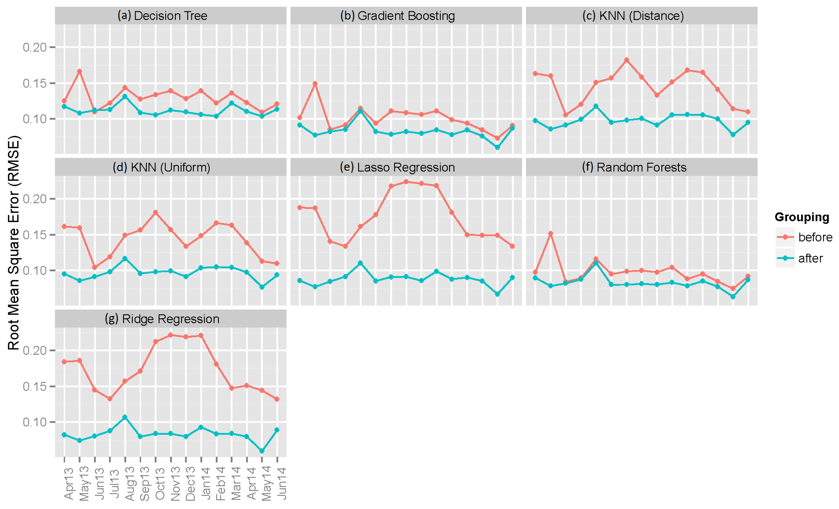
6.2. Individual Machine Learning Models

Figure 5 and Figure 6 show the RMSE and MAE values for the point forecasts from the seven individual machine learning-based regression models. It can be observed that in almost all cases, machine learning-based regression models beat the benchmark models both for before and after grouping of the data by hours of the day (note: if the data are not grouped by hours of the day, the hour is added as an additional (13-th) input variable). It can be seen that grouping helps improve the accuracy of the outputs for the machine learning models, as well. Among all of the regression models, the gradient boosting algorithm offers the best results in terms of average RMSE and MAE.

As in the case of the benchmark models, the probabilistic forecasts by the seven individual regression models can be computed by generating 99 percentiles. Their pinball loss scores are given in Figure 7. The KNN (uniform) method offers the smallest average pinball loss.

The average RMSE, MAE and pinball loss scores of the seven machine learning methods are given in Table 1.

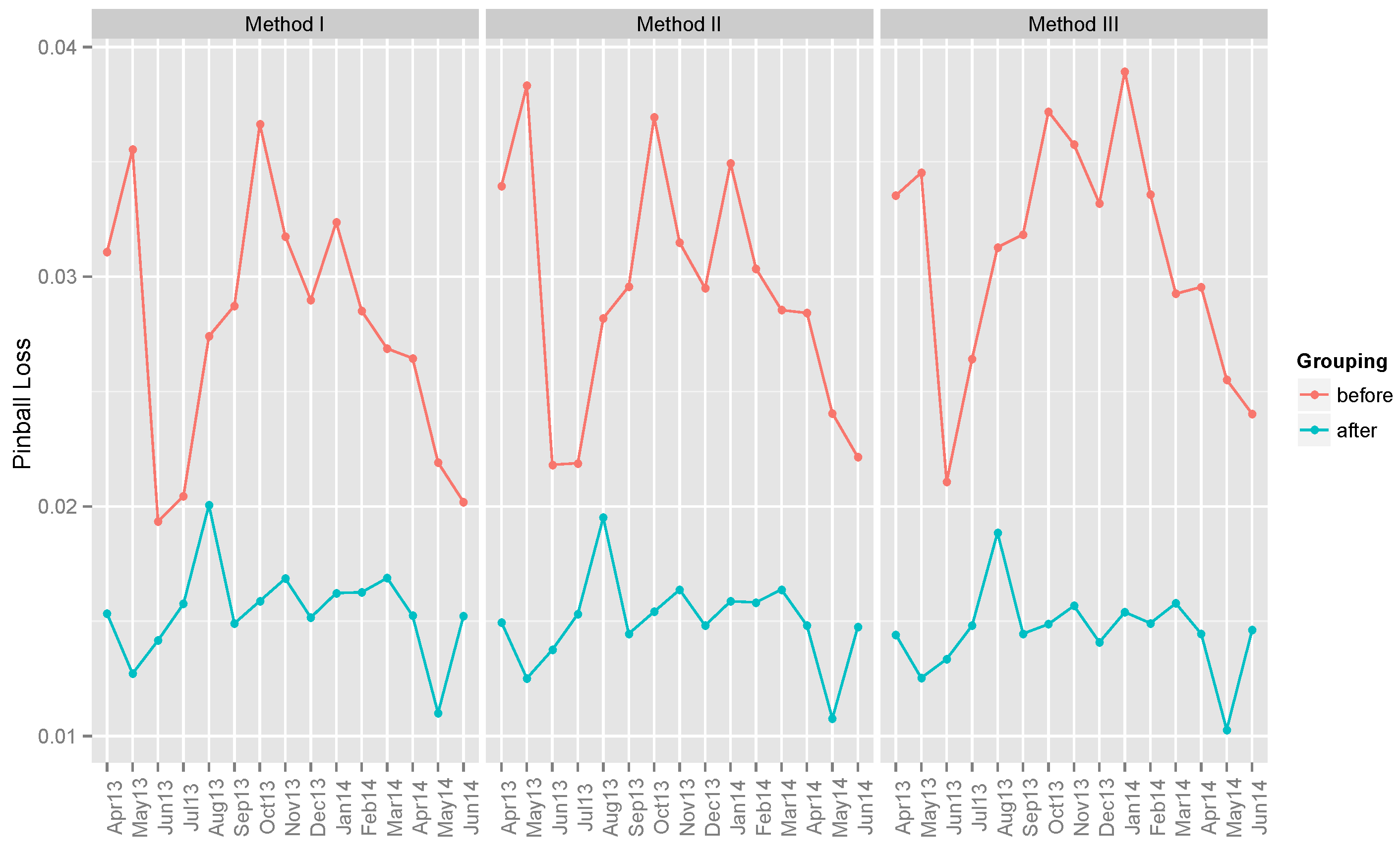
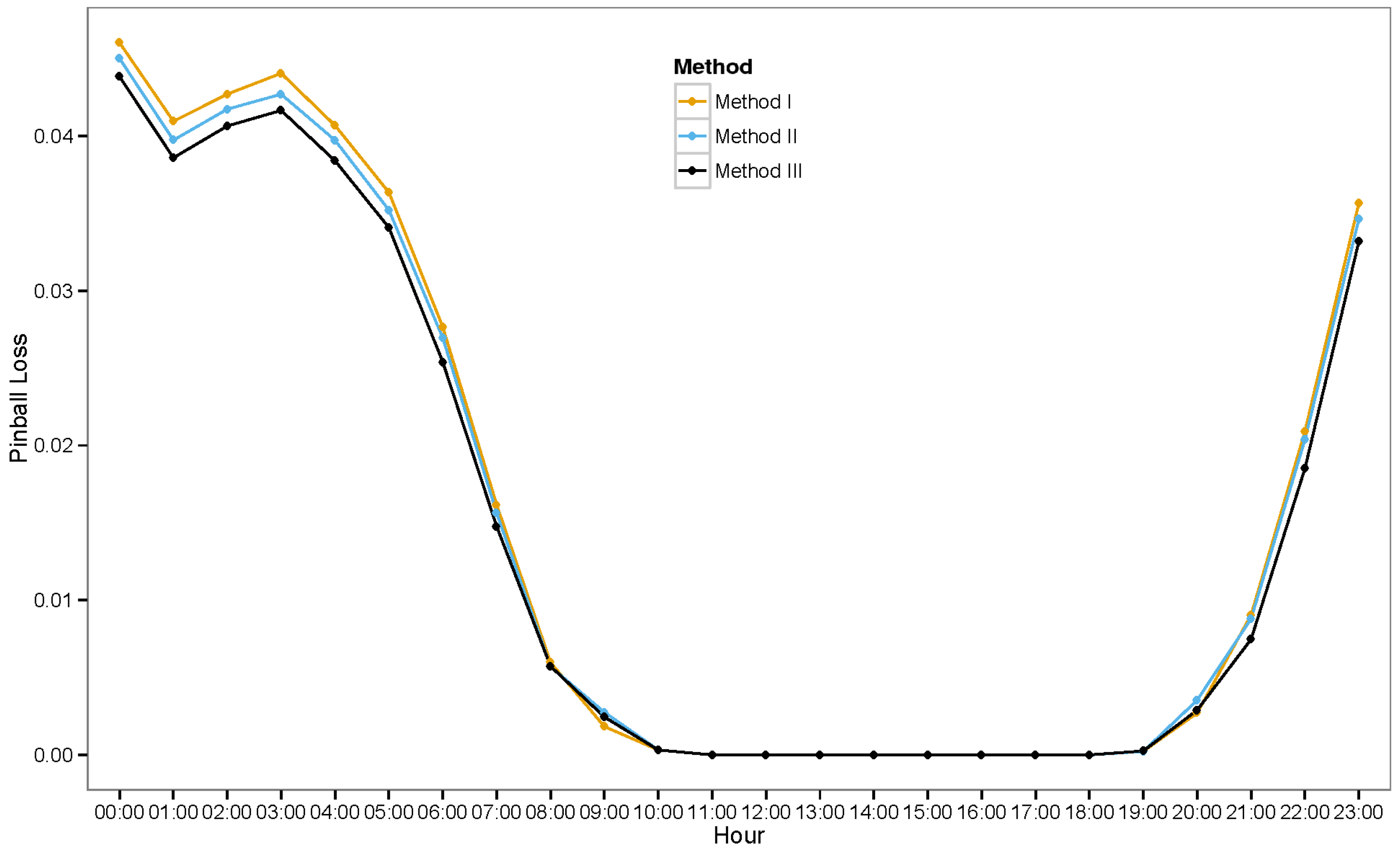
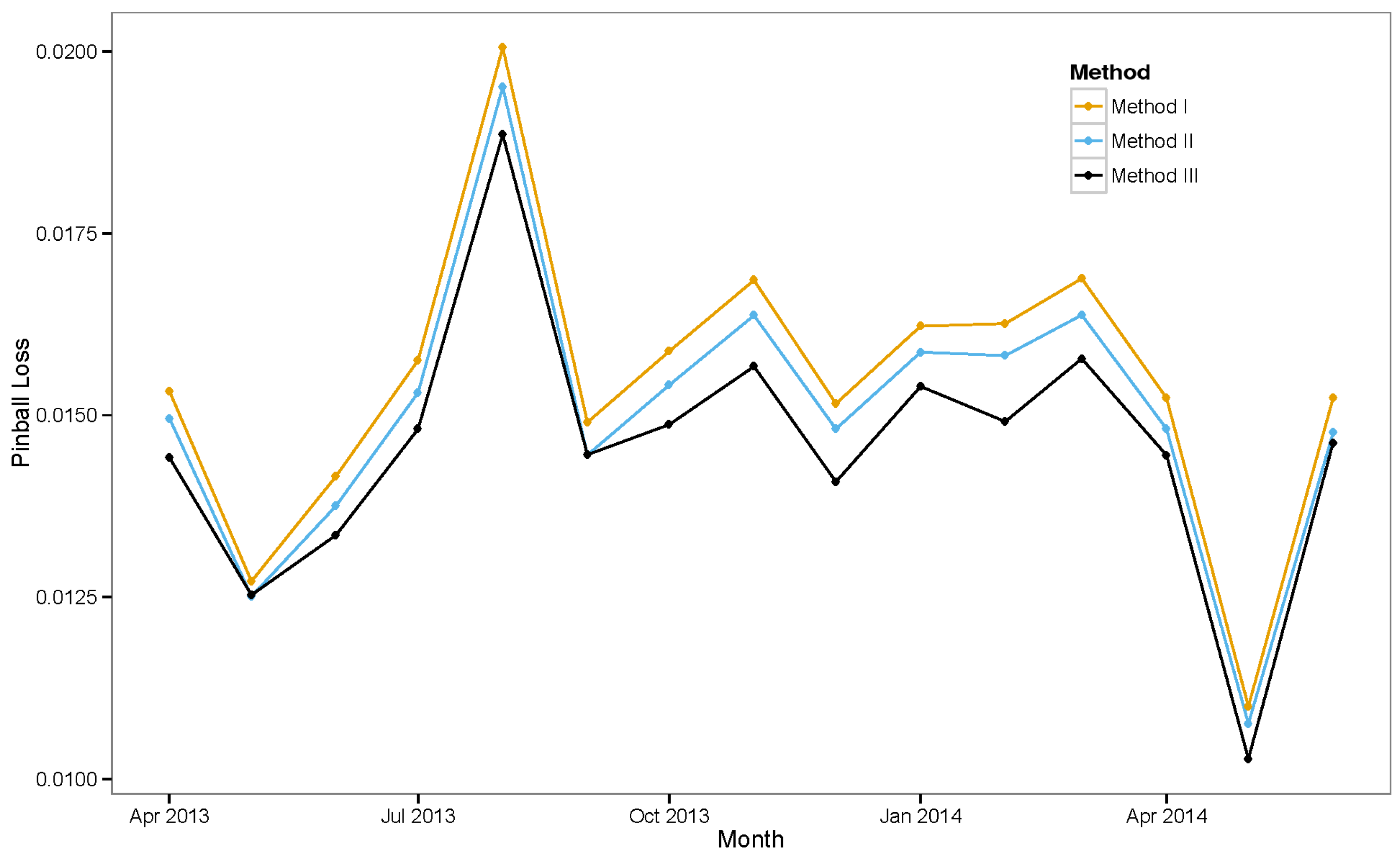
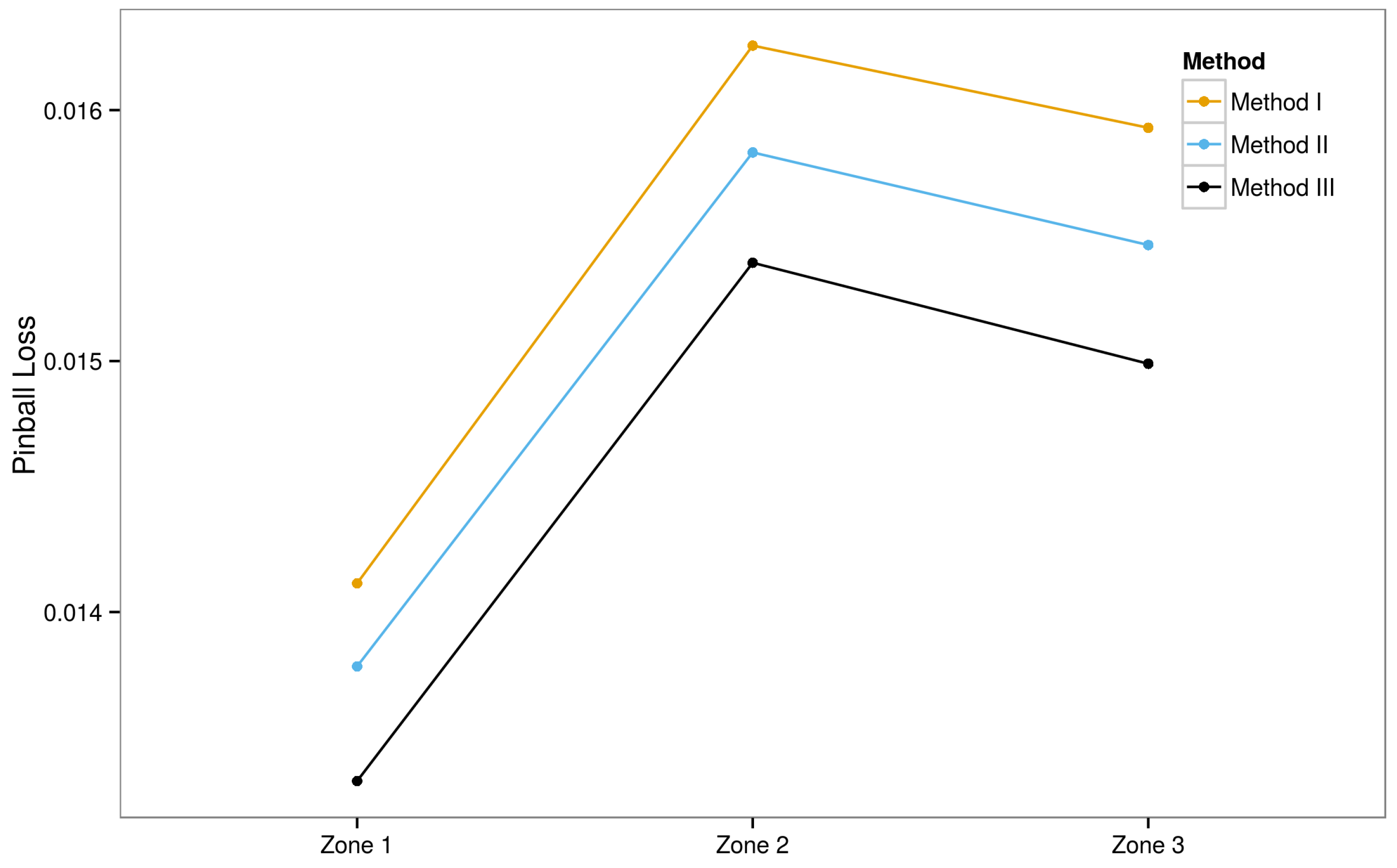
6.3. Ensemble Models

Figure 8 shows the pinball loss scores for the probabilistic forecasts of all three proposed ensemble models before and after grouping by hours of the day (note: we cannot simply use the RMSE and MAE metrics to evaluate probabilistic forecasts, as they are designed just for point forecasts). In comparison with the results by individual regression models in Figure 7, all of the ensemble models help improve the accuracy of the forecasts significantly. Again, it can be seen that the performance has vastly improved after grouping of the data. Method III provides the best results of the three models with an average pinball loss score of 0.01457 when compared to 0.01544 and 0.01503 of Methods I and II, respectively.

Table 1 summarizes Figure 2, Figure 3, Figure 4, Figure 5, Figure 6, Figure 7 and Figure 8, showing the average RMSE, MAE and pinball loss scores for the three benchmark models, the seven individual machine learning models and the three ensemble models.

The average hourly error values in terms of pinball loss scores (after grouping) for the 24 h are shown in Figure 9. Those values vary significantly except for Hours 11 to 18 showing a zero error value since the power generated during that period is zero. The highest error values are observed during Hours 0 through 4.

The average monthly pinball loss scores (after grouping) from April 2013 to June 2014 are shown in Figure 10. Very low errors are observed in the months of May and June, whereas August exhibits the highest error rate. These fluctuations in the error rates are possibly caused by the cloud cover. In general, the better forecasts are achieved in the summer because of clear sky, and there are higher error rates during the winter with more cloud cover during the daytime.

The average zonal pinball loss scores (after grouping) of the three zones (solar farms) are shown in Figure 11. Among the three zones, we obtain the best results for Zone 1, while the results for Zone 2 are the worst for all of the methods. We can observe that there is a rough correlation between the nominal power output of the solar farm (see Section 3) and the pinball loss scores. The smaller the power output of the solar farm, the lower the forecasting error rate.

6.3.1. Ensemble Method III

Among the three ensemble models, it is observed that Ensemble Method III offers the best overall results as shown in Figure 8 and summarized in Table 1. As described in Section 4.3.3, Method III is made up of two added additional sets of regression models along with the original model set of Method II. The first additional model set uses the additional feature “month” of the year along with the existing 12 features, and the second additional model set uses only the most recent 30 days of data (instead of the whole available training data).

It is observed that the contributions of all three sets (the original and the two additional sets) are essential for the good performance of Method III. The relative performances of Method III’s three regression model sets individually and any combinations thereof are given in

Table 2. Performances of three individual sets and any combinations thereof of Method III (in terms of the average pinball loss score after grouping by hours of the day).

Contributor	Pinball Loss
original set only (i.e., Method II)	0.01503
1st additional set only	0.01516
2nd additional set only	0.01794
original set + 1st additional set	0.01510
original set + 2nd additional set	0.01498
1st additional set + 2nd additional set	0.01483
original set + 1st additional set + 2nd additional set (i.e., Method III)	0.01457

.

An example of probabilistic forecasting output by Method III along with the actual solar power generated for a 72-h period (25 May, 0 h to 27 May, 23 h in the year 2013) in Zone 1 is illustrated in Figure 12. For the sake of simplicity, only the 1st, 50th and 99th percentile forecasted values are shown (instead of showing all the first to 99th percentile values).

7. Conclusions

In this study, we explore the concept of generating probabilistic forecasts for solar power output using individual point forecasts from different machine learning models. Day ahead forecasts are generated for three solar farms for a period of 15 months. The models are built using the meteorological data from the European Centre for Medium-Range Weather Forecasts (ECMWF)’s numerical weather prediction (NWP) output provided through the GEFCOM 2014 [22] organizers. The study sought to answer the following questions:

• Does combining the results from different models improve the performance?
• Does grouping the data from each hour and running separate models on them give a better performance?

The findings of this study show that combining the results from individual machine learning-based regression models gave exceedingly better performance than the individual models themselves. These results are consistent across the forecasting horizon of 15 months. Furthermore, grouping the data based on individual hours of the day results in lower error rates in comparison to the results where the data are not grouped. We use three different strategies to combine the results to generate probabilistic forecasts. It is found that Method III, which assumes the normal probability distribution and incorporates additional features, offers the best results.

The field of probabilistic forecasts is still new, and various evaluation metrics are still being developed. In this study, we have used RMSE and MAE to evaluate the point forecasts and pinball loss score to evaluate the probabilistic forecasts. To better evaluate the model, there is a need to explore various other metrics in the field of probabilistic forecasts, like the continuous rank probability score (CRPS). Furthermore, the models can be further improved by relaxing the assumption that the probabilistic forecasts follow a normal distribution, as this assumption is too restrictive.

References

1. Davidson, D.J.; Andrews, J. Not all about consumption. Science 2013, 339, 1286–1287. [Google Scholar] [CrossRef] [PubMed]
2. International Energy Agency. International Energy Outlook 2013. Available online: http://www.eia.gov/forecasts/archive/ieo13 (accessed on 1 November 2016).
3. Goldemberg, J.; Johansson, T.B.; Anderson, D. World Energy Assessment Overview: 2004 Update; United Nations Development Programme, Bureau for Development Policy: New York, NY, USA, 2004. [Google Scholar]
4. International Energy Agency. Technology Roadmap: Solar Photovoltaic Energy. 2014. Available online: http://www.iea.org/publications/freepublications/publication/technology-roadmap-solar-photovoltaic-energy---2014-edition.html (accessed on 1 November 2016).
5. Runyon, J. Transparency and Better Forecasting Tools Needed for the Solar Industry. 2012. Available online: http://www.renewableenergyworld.com/rea/news/article/2012/12/transparency-and-better-forecasting-tools-needed-for-the-solar-industry (accessed on 1 November 2016).
6. Iversen, E.B.; Morales, J.M.; Møller, J.K.; Madsen, H. Probabilistic forecasts of solar irradiance using stochastic differential equations. Environmetrics 2014, 25, 152–164. [Google Scholar] [CrossRef] [Green Version]
7. Grantham, A.; Gel, Y.R.; Boland, J. Nonparametric short-term probabilistic forecasting for solar radiation. Sol. Energy 2016, 133, 465–475. [Google Scholar] [CrossRef]
8. Mohammed, A.A.; Yaqub, W.; Aung, Z. Probabilistic forecasting of solar power: An ensemble learning approach. In Proceedings of the 7th International KES Conference on Intelligent Decision Technologies (KES-IDT), Sorrento, Italy, 17–19 June 2015; Volume 39, pp. 449–458.
9. Mohammed, A.A. Probabilistic Forecasting of Solar Power: An Ensemble Learning Approach. Master’s Thesis, Masdar Institute of Science and Technology, Abu Dhabi, UAE, 2015. [Google Scholar]
10. Bacher, P.; Madsen, H.; Nielsen, H.A. Online short-term solar power forecasting. Sol. Energy 2009, 83, 1772–1783. [Google Scholar] [CrossRef] [Green Version]
11. Huang, Y.; Lu, J.; Liu, C.; Xu, X.; Wang, W.; Zhou, X. Comparative study of power forecasting methods for PV stations. In Proceedings of the 2010 IEEE International Conference on Power System Technology (POWERCON), Hangzhou, China, 24–28 October 2010; IEEE: New York, NY, USA, 2010; pp. 1–6. [Google Scholar]
12. Huang, J.; Korolkiewicz, M.; Agrawal, M.; Boland, J. Forecasting solar radiation on an hourly time scale using a Coupled AutoRegressive and Dynamical System (CARDS) model. Sol. Energy 2013, 87, 136–149. [Google Scholar] [CrossRef]
13. Marquez, R.; Coimbra, C.F.M. Forecasting of global and direct solar irradiance using stochastic learning methods, ground experiments and the NWS database. Sol. Energy 2011, 85, 746–756. [Google Scholar] [CrossRef]
14. Hossain, M.R.; Oo, A.M.T.; Shawkat Ali, A.B.M. Hybrid prediction method for solar power using different computational intelligence algorithms. Smart Grid Renew. Energy 2013, 4, 76–87. [Google Scholar] [CrossRef]
15. Zhu, H.; Li, X.; Sun, Q.; Nie, L.; Yao, J.; Zhao, G. A power prediction method for photovoltaic power plant based on wavelet decomposition and artificial neural networks. Energies 2016, 9, 11. [Google Scholar] [CrossRef]
16. Li, Z.; Rahman, S.M.; Vega, R.; Dong, B. A hierarchical approach using machine learning methods in solar photovoltaic energy production forecasting. Energies 2016, 9, 55. [Google Scholar] [CrossRef]
17. Diagne, M.; David, M.; Lauret, P.; Boland, J.; Schmutza, N. Review of solar irradiance forecasting methods and a proposition for small-scale insular grids. Renew. Sustain. Energy Rev. 2013, 27, 65–76. [Google Scholar] [CrossRef]
18. Antonanzas, J.; Osorio, N.; Escobar, R.; Urraca, R.; de Pison, F.J.M.; Antonanzas-Torres, F. Review of photovoltaic power forecasting. Sol. Energy 2016, 136, 78–111. [Google Scholar] [CrossRef]
19. Gneiting, T.; Katzfuss, M. Probabilistic forecasting. Annu. Rev. Stat. Appl. 2014, 1, 125–151. [Google Scholar] [CrossRef]
20. Hong, T. Energy forecasting: Past, present, and future. Foresight 2014, 32, 43–48. [Google Scholar]
21. Hong, T.; Pinson, P.; Fan, S.; Zareipour, H.; Troccoli, A.; Hyndman, R.J. Probabilistic energy forecasting: Global Energy Forecasting Competition 2014 and beyond. Int. J. Forecast. 2016, 32, 896–913. [Google Scholar] [CrossRef] [Green Version]
22. GEFCOM. Global Energy Forecasting Competition 2014 Probabilistic Solar Power Forecasting. 2014. Available online: https://crowdanalytix.com/contests/global-energy-forecasting-competition-2014-probabilistic-solar-power-forecasting (accessed on 1 November 2016).
23. European Centre for Medium-Range Weather Forecasts. 2016. Available online: http://www.ecmwf.int/ (accessed on 1 November 2016).
24. Coiffier, J. Fundamentals of Numerical Weather Prediction; Cambridge University Press: Cambridge, UK, 2012. [Google Scholar]
25. Bell, R.M.; Koren, Y. Lessons from the Netflix prize challenge. ACM SIGKDD Explor. Newsl. 2007, 9, 75–79. [Google Scholar] [CrossRef]
26. Kotsiantis, S.B. Supervised machine learning: A review of classification techniques. Informatica 2007, 31, 249–268. [Google Scholar]
27. Pedregosa, F.; Varoquaux, G.; Gramfort, A.; Michel, V.; Thirion, B.; Grisel, O.; Blondel, M.; Prettenhofer, P.; Weiss, R.; Dubourg, V.; et al. Scikit-learn: Machine learning in Python. J. Mach. Learn. Res. 2011, 12, 2825–2830. [Google Scholar]
28. Breiman, L.; Friedman, J.; Stone, C.; Olshen, R.A. Classification and Regression Trees; Taylor & Francis: Abingdon, UK, 1984. [Google Scholar]
29. Friedman, J.H. Greedy function approximation: A gradient boosting machine. Ann. Stat. 2001, 29, 1189–1232. [Google Scholar] [CrossRef]
30. Altman, N.S. An introduction to kernel and nearest-neighbor nonparametric regression. Am. Stat. 1992, 46, 175–185. [Google Scholar]
31. Tibshirani, R. Regression shrinkage and selection via the lasso. J. R. Stat. Soc. Ser. B (Methodol.) 1996, 58, 267–288. [Google Scholar]
32. Breiman, L. Random forests. Mach. Learn. 2001, 45, 5–32. [Google Scholar] [CrossRef]
33. Hoerl, A.E.; Kennard, R.W. Ridge regression: Biased estimation for nonorthogonal problems. Technometrics 1970, 12, 55–67. [Google Scholar] [CrossRef]
34. Langford, E. Quartiles in elementary statistics. J. Stat. Educ. 2006, 14, n3. [Google Scholar]
35. Larson, R.; Farber, E. Elementary Statistics: Picturing the World; Prentice Hall: Upper Saddle River, NJ, USA, 2003. [Google Scholar]
36. Koenker, R. Quantile Regression; Cambridge University Press: Cambridge, UK, 2005. [Google Scholar]
37. Hyndman, R.J.; Athanasopoulos, G.; Razbash, S.; Schmidt, D.; Zhou, Z.; Khan, Y.; Bergmeir, C.; Wang, E. Forecast: Forecasting Functions for Time Series and Linear Models. R Package Version 5.6. 2014. Available online: http://CRAN.R-project.org/package=forecast (accessed on 1 November 2016).
38. R Core Team. R: A Language and Environment for Statistical Computing; R Foundation for Statistical Computing: Vienna, Austria, 2014; Available online: http://www.R-project.org/ (accessed on 1 November 2016).
39. Hyndman, R.J.; Athanasopoulos, G. Forecasting: Principles and Practice; OTexts: Toronto, ON, Canada, 2013. [Google Scholar]
Figure 1. Observed solar power values for the month of April 2012 in Zone 1.
Energies 09 01017 g001
Figure 2. Average RMSE values of benchmark models’ point forecasts before and after grouping of data by hours of the day.
Energies 09 01017 g002
Figure 3. Average MAE values of benchmark models’ point forecasts before and after grouping of data by hours of the day.
Energies 09 01017 g003
Figure 4. Average pinball loss scores of benchmark models’ point forecasts before and after grouping of data by hours of the day.
Energies 09 01017 g004
Figure 5. Average RMSE values of seven individual machine learning models’ point forecasts before and after grouping of data by hours of the day. Results for: (a) decision tree; (b) gradient boosting; (c) KNN (distance); (d) KNN (uniform); (e) lasso regression; (f) random forests; and (g) ridge regression.
Energies 09 01017 g005
Figure 6. Average MAE values of seven individual machine learning models’ point forecasts before and after grouping of data by hours of the day. Results for: (a) decision tree; (b) gradient boosting; (c) KNN (distance); (d) KNN (uniform); (e) lasso regression; (f) random forests; and (g) ridge regression.
Energies 09 01017 g006
Figure 7. Pinball loss scores of seven individual machine learning models’ point forecasts before and after grouping of data by hours of the day. Results for: (a) decision tree; (b) gradient boosting; (c) KNN (distance); (d) KNN (uniform); (e) lasso regression; (f) random forests; and (g) ridge regression.
Energies 09 01017 g007
Figure 8. Pinball loss scores of three ensemble models’ probabilistic forecasts before and after grouping of data by hours of the day.
Energies 09 01017 g008
Figure 9. Average pinball loss scores for different hours. (Note: the hours shown on the X-axis are just nominal and not the real wall-clock hours. The offset between these two is not disclosed by the Global Energy Forecasting Competition (GEFCOM) 2014 organizers.)
Energies 09 01017 g009
Figure 10. Average pinball loss scores for different months.
Energies 09 01017 g010
Figure 11. Average pinball loss scores for different zones (solar farms).
Energies 09 01017 g011
Figure 12. Example of probabilistic forecasting by Method III. First, 50th and 99th percentile forecasted values are shown along with actual solar power generated for the 72-h period (25 May, 0 h to 27 May, 23 h in year 2013) in Zone 1.
Energies 09 01017 g012