Study of Wind Turbine Fault Diagnosis Based on Unscented Kalman Filter and SCADA Data

Abstract

Effective wind turbine fault diagnostic algorithms are crucial for wind turbine intelligent condition monitoring. An unscented Kalman filter approach is proposed to successfully detect and isolate two types of gearbox failures of a wind turbine in this paper. The state space models are defined for the unscented Kalman filter model by a detailed wind turbine nonlinear systematic principle analysis. The three failure modes being studied are gearbox damage, lubrication oil leakage and pitch failure. The results show that unscented Kalman filter model has special response to online input parameters under different fault conditions. Such property makes it effective on fault identification. It also shows that properly defining unscented Kalman filter state space vectors and control vectors are crucial for improving its sensitivity to different failures. Online fault detection capability of this approach is then proved on SCADA data. The developed unsented Kalman filter model provides an effective way for wind turbine fault detection using supervisory control and data acquisition data. This is essential for further intelligent WT condition monitoring.

1. Introduction

Accurate and reliable wind turbine (WT) condition monitoring system (CMS) is important for wind farm reliability centre maintenance that is expected to increase WT availability and decrease cost of wind energy [1,2]. Developing effective WT fault diagnostic algorithms are crucial for reliable WT CMS. Due to the variable-speed operation of a WT and stochastic characteristics of load, traditional frequency domain techniques for WT fault detection may not be applicable. There has been increasing trend of developing model based algorithm for fault detection and isolation [3]. Typically, CMS analyses high frequency signals such as vibrations in frequency domain to monitor WT health while its cost per channel is high. Supervisory control and data acquisition (SCADA) system mounted in the WT controller to allow local and remote control of basic WT functions by collecting WF data is originally used to analyze and report on operational performance. Its signal sampling rate and data storage requirement are low and then its cost is lower compare to CMS [4]. However, low frequency characteristics of SCADA data were considered to have low accuracy and may lead to challenge of using it on fault diagnosis. Recently, Qiu YN and Feng YH [4,5] prove the relationship between the SCADA data trending and WT failures based on physical principle analysis, which reveals that for certain failure modes SCADA data is useful on the fault detection and diagnosis. Fault features can be captured by anomaly detection algorithms developed on SCADA data [6].

Earliest attempt to use SCADA data on WT fault detection is using neural network technique to realize automated anomaly detection on signals [7]. Thereafter, different signal processing techniques have been applied to develop appropriate algorithm for accurate fault detection and diagnosis [8,9,10,11]. The signals used for WT fault detection include vibration, acoustic emission, strain, torque, temperature etc. They range from mechanical signal to electrical signals. The signal processing methods used for fault feature mining include time-domain method, classical frequency analysis method, time-frequency analysis methods, model based method, probability-based method, artificial intelligent method etc. [8]. Although comparison of different approaches, such as signal trending, self-organizing maps and physical model, on using SCADA data for fault detection shows that physical model has superior performance [12,13] on fault isolability, identificability, its dependence on modelling and poor robustness make it difficult for implementation. Recently, Philip C [14] develops an adaptive data-driven wind turbine model for fault detection and demonstrates its success on implementation. However, data driven approach also has problem on providing explanation on fault origins, which will lead to poor capability on fault isolation. This is also main issue for artificial intelligent approaches, which cannot provide convincing explanation for various fault features. Sataru [15] uses model based cascaded Kalman filter to show its advances on fault detection and isolation while the nonlinearity of WT system is solved by nonlinear map. This indicates increasing trend of using model-based approaches for WT fault detection.

This paper proposed a quantitative model-based approach for WT online fault detection and diagnosis. It is realized by constructing a cascaded unscented Kalman filter (UKF) model by operational principle analysis. Previous researches of WT gearbox degradation and generator faults clarify the failure mechanisms [16,17] and offer a reference for WT quantitative model development. In addition, considering the nonlinear characteristics of a WT system cascaded UKF is adopted [18,19]. The health status of a wind turbine is judged by comparison of UKF prediction results and simulation results under the same input. The prediction results of the WT with fault deviate from simulation results. The location and detection of faults are achieved based on residual trending. Its fault detection performances are then evaluated in terms of fault detection capability.

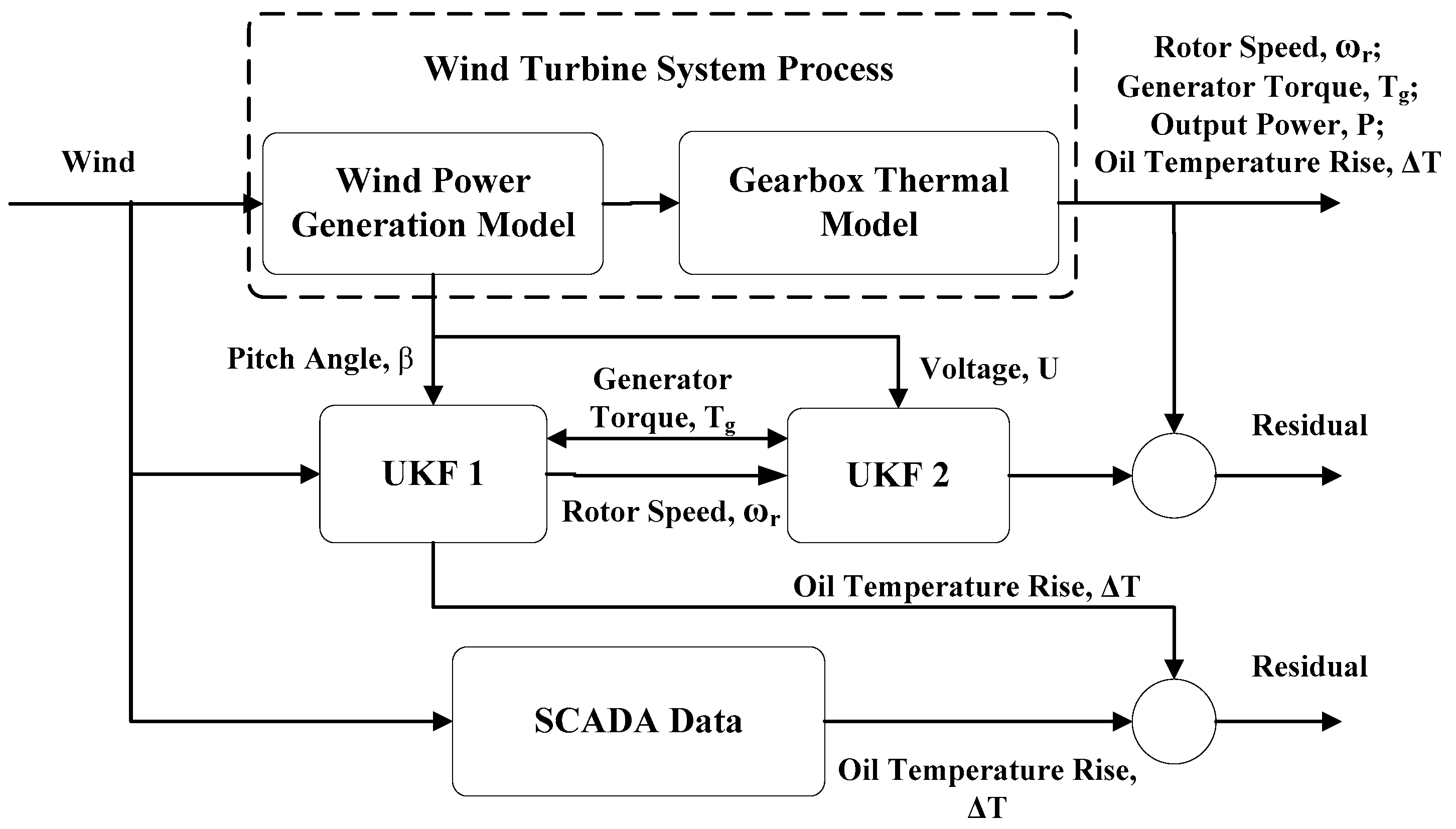
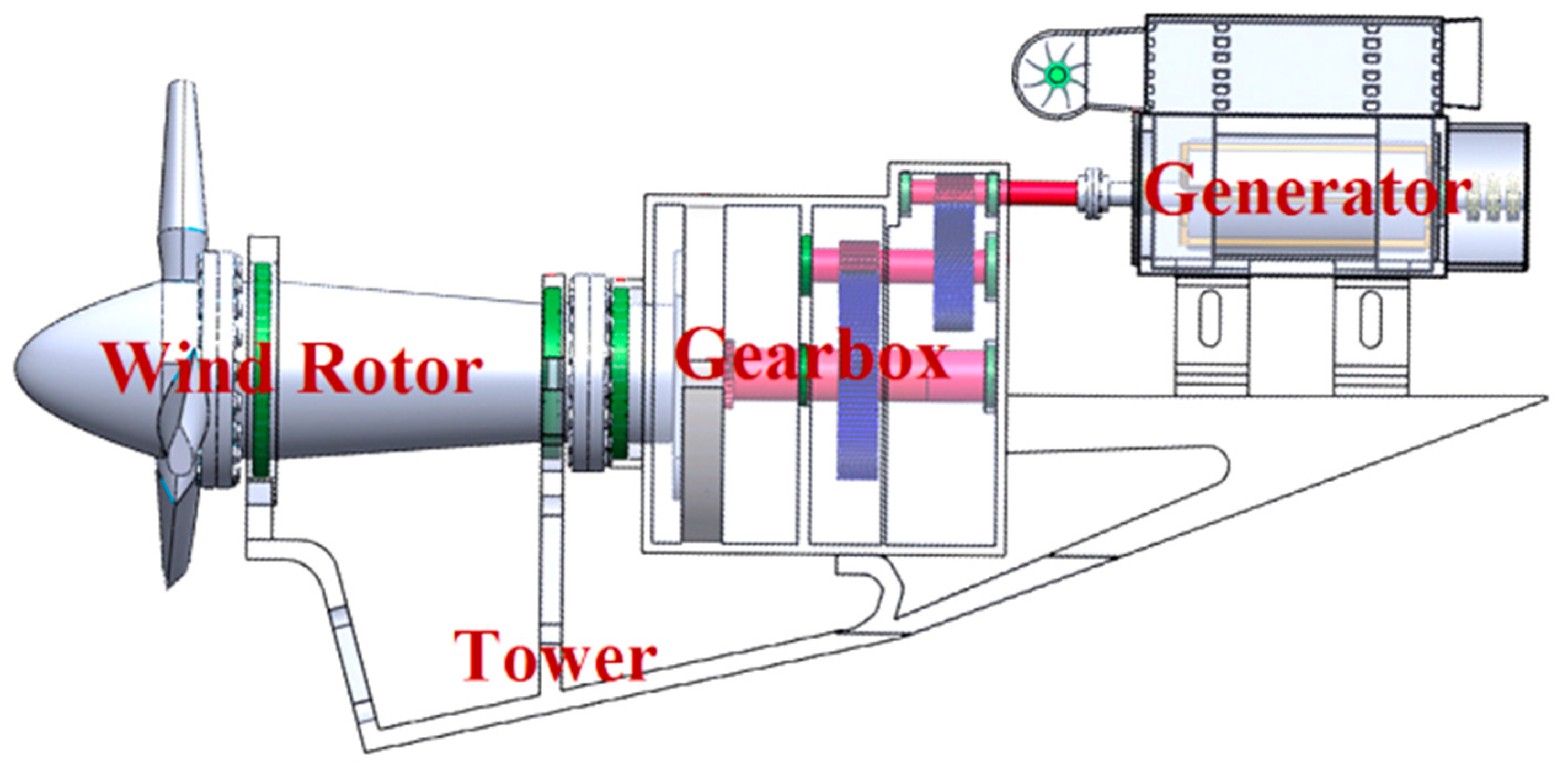
2. System Model

Figure 1 illustrates the process of developing a quantitative model-based fault diagnostic algorithm and also the structure of this paper. The wind turbine operational process is firstly presented by two main process, wind power generation model and gearbox thermal model. The wind turbine model simulates systematic output under healthy and faulty situation. According to the WT operational principle, a cascaded UKF model is developed to detect three faults: gearbox damage, oil leakage and pitch failure. Residuals between predicted results and simulation outputs for the three failure modes are compared and discussed. Then the predicted results of UKF model are further compared to SCADA data. Its effectiveness is finally evaluated and summarized in terms of fault detection capability criteria.

2.1. Wind Power Generation Model

As illustrated in Figure 2, the wind turbine system studied in this paper is 1.5–2 MW with typical configuration of wind rotor, electrical pitch, gearbox, doubly fed induction generator, tower etc. The wind rotor is driven by the mechanical energy from input wind. The rotational speed of the spindle is controlled jointly by input mechanical torque and the reverse torque generated by the generator. The generator’s electromagnetic torque is controlled by the stator voltage to realize maximum power point tracking when wind speed is under rated range. If wind speed is above rated, pitch system controls pitch angle to limit the input mechanical energy in order to maintain constant output power. The WT operational principle was discussed and the simulation models was developed in [16,17]. The simulation is performed according to a WT with 1.5–2 MW, which is configured with a gearbox and doubly fed induction generator. Its simulation model is constructed according to WT’s steady state rotor aerodynamics, simplified drive train aerodynamics and control principles as discussed in [16,17]. The time domain simulation result is obtained according to wind speed variation as input to the model.

2.2. Gearbox Thermal Model

WT energy efficiency is determined by the amount of energy loss during the transmission process within the drive train. Part of energy loss will dissipate within the gearbox in the form of heat due to the bearing friction, gear meshing, oil mixing and viscous friction [16,20]. To simplify the calculation, this paper assumes that the energy loss in the process of gearbox transmission dissipated as heat through three ways [16,21]: heat conduction and convection to the external environment from the gearbox, $Q_1$; heat exchange by oil supplied via the oil cooling system, $Q_2$; heat loss to the adjacent components by conduction through the coupling shaft, base and all internal components, $Q_3$. The gearbox thermal model is developed by lumped parameter approach as shown in Equation (1), with assumption that thermal equilibrium is reached in the gearbox.

$$\{\begin{array}{l}{Q}_{loss}=Q_1+Q_2+Q_3\\ Q_1=KA\Delta T\\ Q_2=c_1\mathsf{\rho }q\Delta T\\ Q_3=c_{2}m\Delta T\end{array}$$

(1)

where $K$ is the overall heat transfer coefficient, calculated by $K=1/(1/h_1+L/k+1/h_2)$ [21], where $h_1$ and $h_2$ are the convective heat transfer coefficient of oil and air; $k$ is the thermal conductivity of gearbox casing; $L$ is the thickness of gearbox casing; $A$ is the surface area of the gearbox casing; $c_1$, $\mathsf{\rho }$, $q$ are the specific heat capacity, density and flow rate of cooling oil; $c_2$ and $m$ are the specific heat capacity and mass of gearbox; $\Delta T$ is the gearbox temperature-rise.

2.3. Unscented Kalman Filter Model

A cascaded UKF method is developed based on the analysis in Section 2.1. and Section 2.2. UKF method matches nonlinear distribution with the sampling strategy [22], which has better applicability in nonlinear system comparing to the traditional linearization method. The core of UKF is unscented transform (UT) [19,23]: For n-dimensional random variable $x$, which has the mean value $\overline{x}$ and covariance $P_x$, a group of sigma points ($\mathsf{\sigma }$) is available for nonlinear transform of every sigma point. The optimal state estimation and covariance can be obtained through statistics for the transformed sigma points. For the following nonlinear discrete time dynamic system:

$$X(k+1)=f[X(k),u(k)]+O(k)$$

(2)

$$Y(k)=h[X(k)]+M(k)$$

(3)

where X(k) is the state; u(k) is the inputs; Y(k) is the measurement outputs; f and h are system function and measurement function; O(K) and M(k) are process noise and measurement noise. The sigma points and weights can be made as follows:

$$\{\begin{array}{l}{\mathsf{\sigma }}_0=\overline{x}\\ {\mathsf{\sigma }}_i=\overline{x}+{[\sqrt{(n+\mathsf{\lambda })P_x}]}_i,i=1,\dots ,n\\ {\mathsf{\sigma }}_i=\overline{x}-{[\sqrt{(n+\mathsf{\lambda })P_x}]}_{i-n},i=n+1,\dots ,2n\end{array}$$

(4)

$$\{\begin{array}{l}{W}_0^m=\mathsf{\lambda }/(n+\mathsf{\lambda })\\ W_0^c=\mathsf{\lambda }/(n+\mathsf{\lambda })+1-{\mathsf{\alpha }}^2+\mathsf{\beta }\\ W_i^m=W_i^c=1/2(n+\mathsf{\lambda }),i=1,\dots ,2n\end{array}$$

(5)

$$\lambda ={\mathsf{\alpha }}^2(n+k)-n$$

(6)

where $k\ge 0$ is to ensure positive semi-definite covariance matrix; $\mathsf{\alpha }$ determines the distribution of sigma points, $0\le \mathsf{\alpha }\le 1$; $\mathsf{\beta }=2$ for Gaussian Noise.

Due to complexity of a WT system monitoring all of its state parameters will consume large amount of resources. To improve the efficiency of fault diagnosis, cascaded UKF model is defined for two subsystems of a WT in order to reduce the number of state parameters and avoid complex mathematical description of the control system. In addition, WT system is a time-varying nonlinear system, its process function is not the typical form of linear equation. The first stage $f_1$ in the UKF system model contains the aerodynamics of wind rotor, gearbox mechanics and thermal mechanism, which predicts the rotor speed ${\mathsf{\omega }}_r$ and temperature-rise of the gearbox $\Delta T$ with controlled vector of wind speed $v$ and pitch angle $\mathsf{\beta }$ from WT system process. The second stage $f_2$ is the generator model, which predicts the generator electromagnetic torque $T_g$ with the controlled vector of voltage $U$ and the rotational speed ${\mathsf{\omega }}_r$ obtained from WT system process and the first stage UKF model respectively. The nonlinear system equations and its state space vectors are expressed as Equations (7)–(10):

$$\{\begin{array}{l}{X}_1={[{\mathsf{\omega }}_r,\Delta T]}^{\mathrm{T}}\\ u_1={[v,\mathsf{\beta }]}^{\mathrm{T}}\end{array}$$

(7)

$$\{\begin{array}{l}{[{\dot{\mathsf{\omega }}}_r,\Delta T]}^{\mathrm{T}}=[g_1({\mathsf{\omega }}_r,v,\mathsf{\beta }),g_2(v,\mathsf{\beta })]+O_1\\ g_1({\mathsf{\omega }}_r,v,\mathsf{\beta })=\left[0.5{\mathsf{\pi }\mathsf{\rho }}_0{R}^2{v}^3{C}_p({\mathsf{\lambda }}_0,\mathsf{\beta })/{\mathsf{\omega }}_r-N{T}_g/\mathsf{\eta }\right]/\left(J_r+N^2{J}_g/\mathsf{\eta }\right)\\ g_2(v,\mathsf{\beta })=(1-\mathsf{\eta })0.5{\mathsf{\pi }\mathsf{\rho }}_0{R}^2{v}^3{C}_p({\mathsf{\lambda }}_0,\mathsf{\beta })/(KA+c_1\mathsf{\rho }q+c_{2}m)\\ {\mathsf{\lambda }}_0={\mathsf{\omega }}_{r}R/v\end{array}$$

(8)

$$\{\begin{array}{l}{X}_2=T_g\\ u_2={[{\mathsf{\omega }}_r,U]}^{\mathrm{T}}\end{array}$$

(9)

$$\{\begin{array}{l}{T}_g=g_3({\mathsf{\omega }}_r,U)+O_2\\ g_3({\mathsf{\omega }}_r,U)=p_1{m}_1{U}^2{r}_r/\{(N{\mathsf{\omega }}_r-{\mathsf{\omega }}_1)[{(r_s-C{r}_r{\mathsf{\omega }}_1/(N{\mathsf{\omega }}_r-{\mathsf{\omega }}_1))}^2+{(x_s+C{x}_r)}^2]\}\end{array}$$

(10)

where $T_r$ is the torque of low speed shaft; ${\mathsf{\rho }}_0$ is air density; $R$ is the wind rotor radius; $C_p$ is wind power coefficient, determined by the tip speed ratio ${\mathsf{\lambda }}_0$ and pitch angle $\mathsf{\beta }$; $J_r$ and $J_g$ are the rotational inertia of WT rotor and generator; $N$, $\mathsf{\eta }$ are the drive ratio and transmission efficiency of gearbox; ${\mathsf{\omega }}_r$, ${\mathsf{\omega }}_g$, ${\mathsf{\omega }}_1$ are rotor speed, generator speed and synchronous speed; $p_1$ and $m_1$ are the pole number and phase number of a generator; $r_s$, $r_r$, $x_s$ and $x_r$ are generator parameters of generator stator and rotor; $C$ is the correction factor.

The unscented transformation are described as:

$${\mathsf{\gamma }}_i(k+1)=f[{\mathsf{\sigma }}_i(k),u(k)]$$

(11)

and the priori state estimation and covariance are calculated by:

$$\widehat{X}(k+1)={\displaystyle \sum _{i=0}^{2n}{W}_i^m}{\mathsf{\gamma }}_i(k+1)$$

(12)

$$P_x^{-}(k+1)={\displaystyle \sum _{i=0}^{2n}{W}_i^c[{\mathsf{\gamma }}_i(k+1)-\widehat{X}(k+1)]{[{\mathsf{\gamma }}_i(k+1)-\widehat{X}(k+1)]}^{\mathrm{T}}}+O(k)$$

(13)

For the measurement update step, taking the power as measurement variable, the measurement output and covariance are calculated by:

$$y_i(k+1)=h[{\mathsf{\gamma }}_i(k+1)]$$

(14)

$$\widehat{Y}(k+1)={\displaystyle \sum _{i=0}^{2n}{W}_i^m}{y}_i(k+1)$$

(15)

$$P_y(k+1)={\displaystyle \sum _{i=0}^{2n}{W}_i^c[y_i(k+1)-\widehat{Y}(k+1)]{[y_i(k+1)-\widehat{Y}(k+1)]}^{\mathrm{T}}}+M(k+1)$$

(16)

The cross covariance between $\widehat{X}(k+1)$ and $\widehat{Y}(k+1)$ is:

$$P_{xy}(k+1)={\displaystyle \sum _{i=0}^{2n}{W}_i^c[{\gamma }_i(k+1)-\widehat{X}(k+1)]{[y_i(k+1)-\widehat{Y}(k+1)]}^{\mathrm{T}}}$$

(17)

The measurement update of the optimal state estimation and covariance are:

$$K(k+1)=P_{xy}(k+1)P_y^{-1}(k+1)$$

(18)

$$X^{+}(k+1)=\widehat{X}(k+1)+K(k+1)[Y(k+1)-\widehat{Y}(k+1)]$$

(19)

$$P_x^{+}(k+1)=P_x^{-}(k+1)-K(k+1)P_y(k+1)K^{\mathrm{T}}(k+1)$$

(20)

The selection strategy of sigma points includes sampling number, location and weight factor. The current strategies used include symmetric sampling, simplex sampling, 3-order skew sampling and 4-order Gaussian sampling [22]. Symmetric sampling is adopted in this paper and the UKF is initialized as follow:

$$\{\begin{array}{l}{X}_0={[X_{1,0},X_{2,0}]}^{\mathrm{T}}={[1.37,0,0]}^{\mathrm{T}}\\ P_0=\text{diag}[{10}^{-2},1,{10}^4]\end{array}$$

(21)

The comparison between UKF model prediction result and simulation result are evaluated through their residuals. The residual is calculated as:

$$S=|{\text{Value}}_{\text{prediction}}-{\text{Value}}_{\text{real}}|$$

(22)

The parameters of the WT model are designed according to a 1.5–2 MW WT, shown as

Table 1. Wind turbine parameters.

Symbol	Quantity	Value
${\mathsf{\rho }}_0$	air density	1.225 kg/m3
R	wind rotor radius	31 m
Jr	rotor rotational inertia	2,460,106 kg∙m2
Jg	generator rotational inertia	52 kg∙m2
N	drive ratio	100
ω1	synchronous speed	157 rad/s
p1	pole number	2
m1	phase number	3
rs	stator resistance	0.029 Ω
rr	converted rotor resistance	0.023 Ω
xs	stator leakage reactance	0.18 Ω
xr	converted rotor leakage reactance	0.18 Ω
C	correction factor	0.811

.

2.4. Fault Injection and Description

The rated wind speed of the 1.5–2 MW WT mentioned above is 12 m/s, its gearbox efficiency in health is 97%, flow rate of gearbox lubrication oil is 0.84 L/s, pitch angle below the rated wind speed is 0°. Three failure modes introduced in the WT simulation model are:

Fault 1:

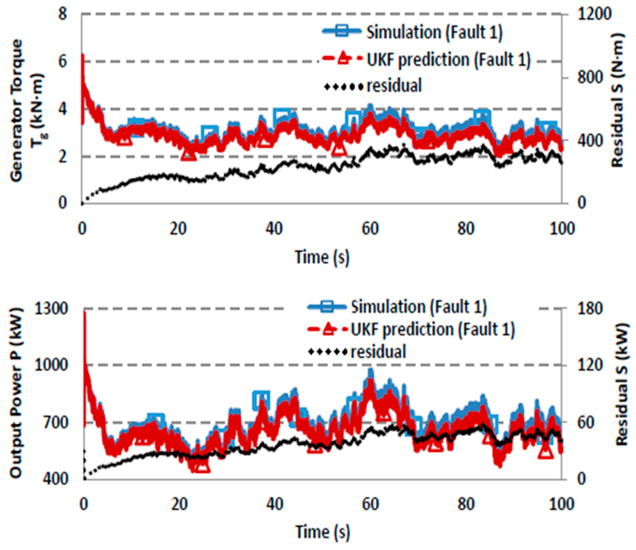
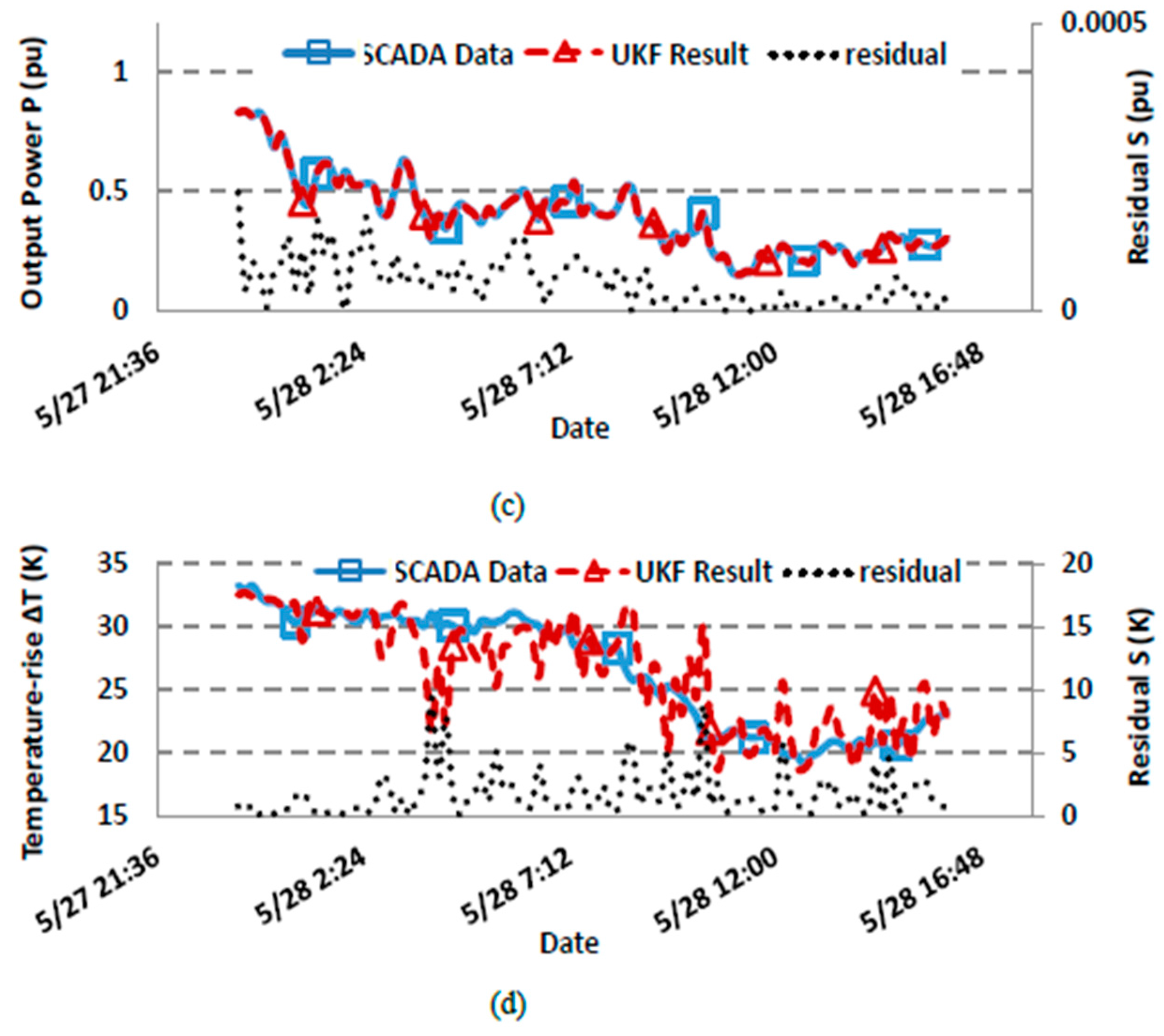
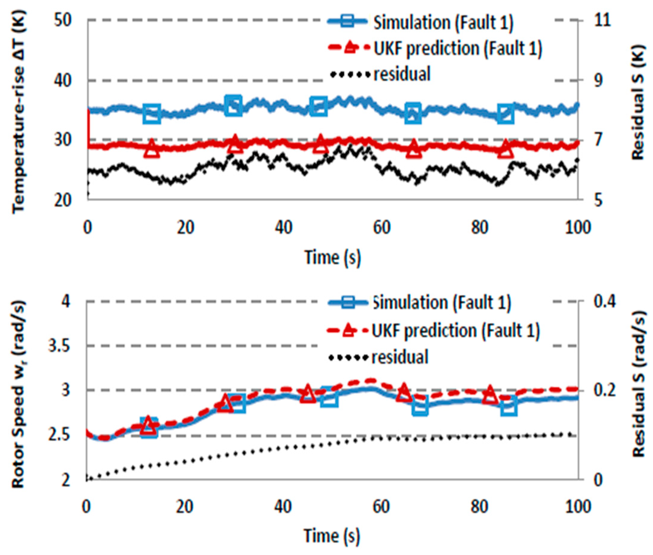
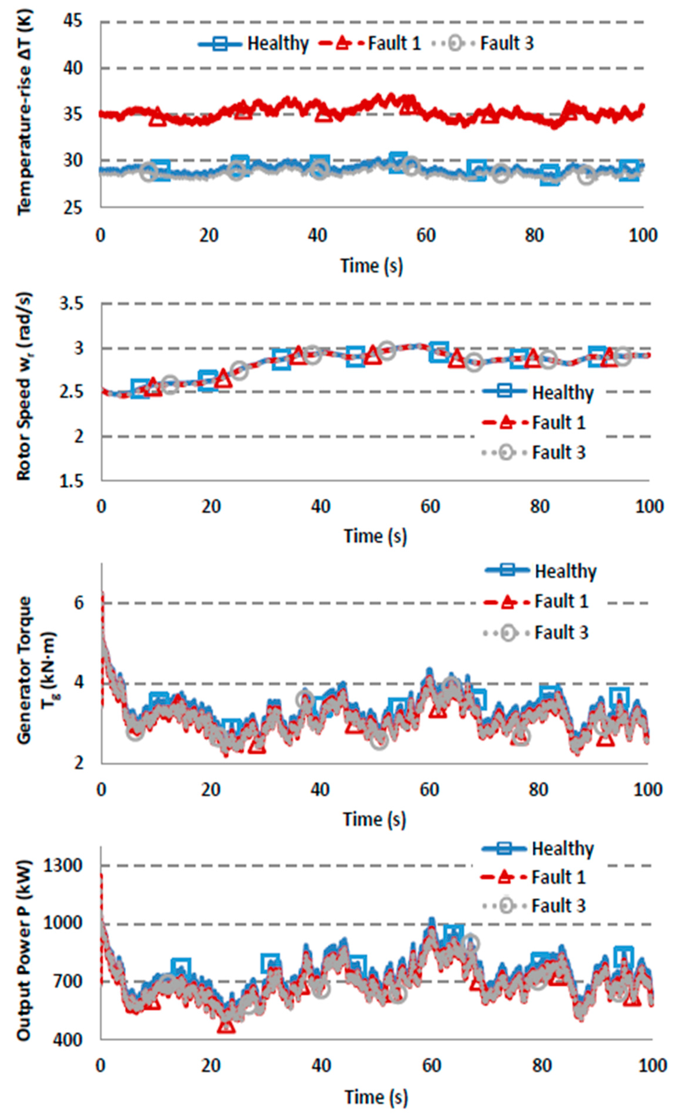
Due to wearing of the gearbox, the mechanical energy transmission efficiency reduces to 92%, which further lead to reduce of output torque and power. Additional losses of energy dissipate as heat in the gearbox, which results in abnormal temperature-rise [16].

Fault 2:

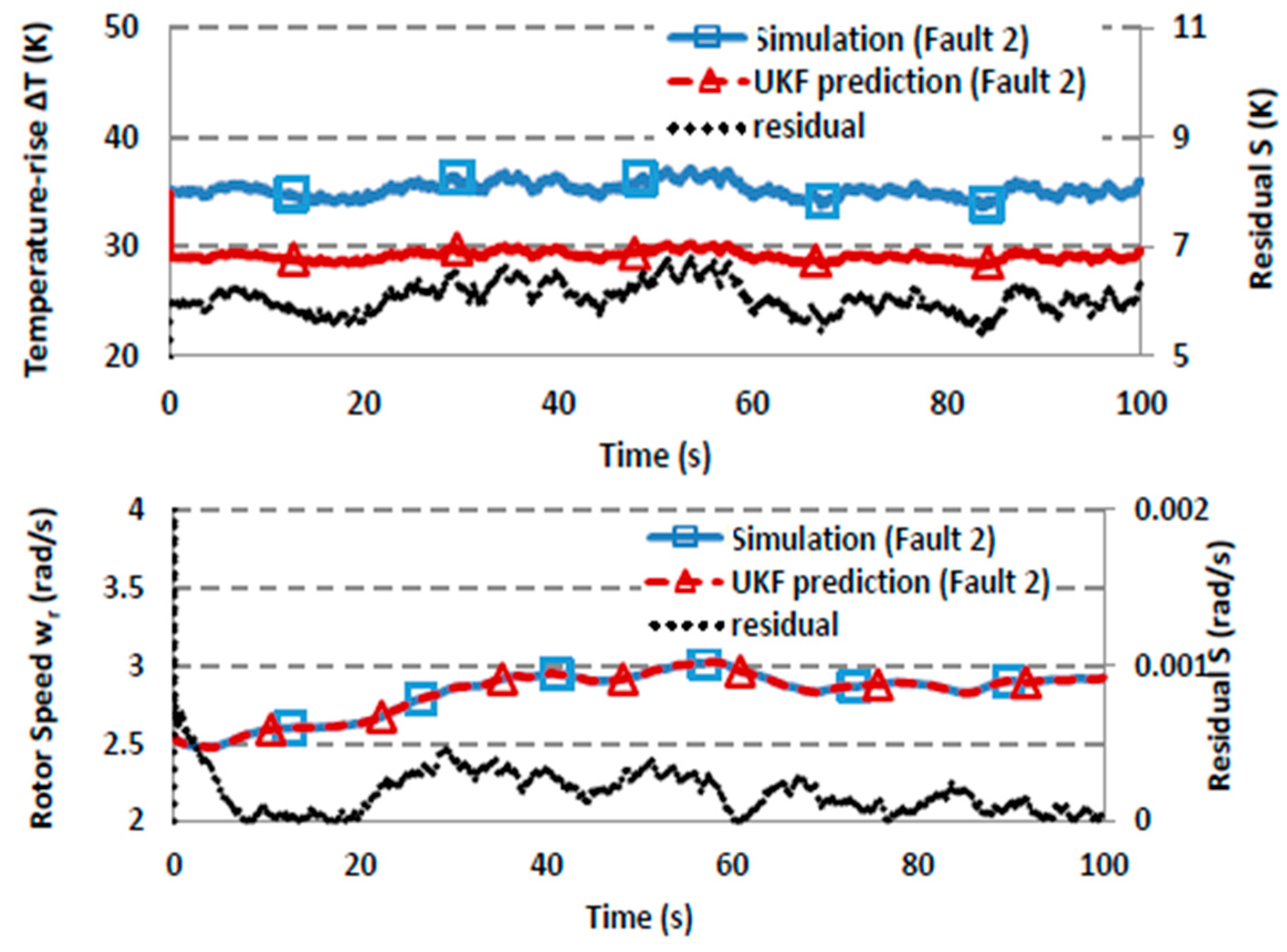
Lubricating oil leakage is a common failure mode of WT. It is assumed that the lubrication oil leakage leads to the reduction of its flow rate from 0.84 L/s to 0.24 L/s. The heat dissipated through lubrication oil is reduced and therefore results in temperature-rise of gearbox.

Fault 3:

This paper simulates pitch system failure by setting pitch angle as 45° when wind speed is below rated wind speed range. Increase of pitch angel will lead to decrease of mechanical energy extracted by WT and then power generation.

With the defined state space vectors Xs and the control vector Us for the first and second UKF model, the predicted rotor speed, generator torque, power and gearbox temperature-rise are obtained. The feasibility of this UKF method on the wind turbine fault diagnosis is discussed through the comparison between predicted and simulated results.

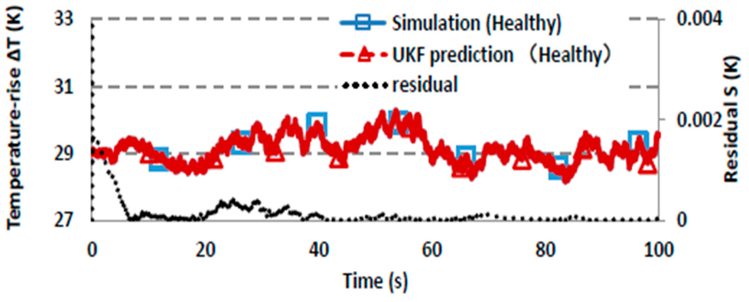
3. Simulation Results and Analysis

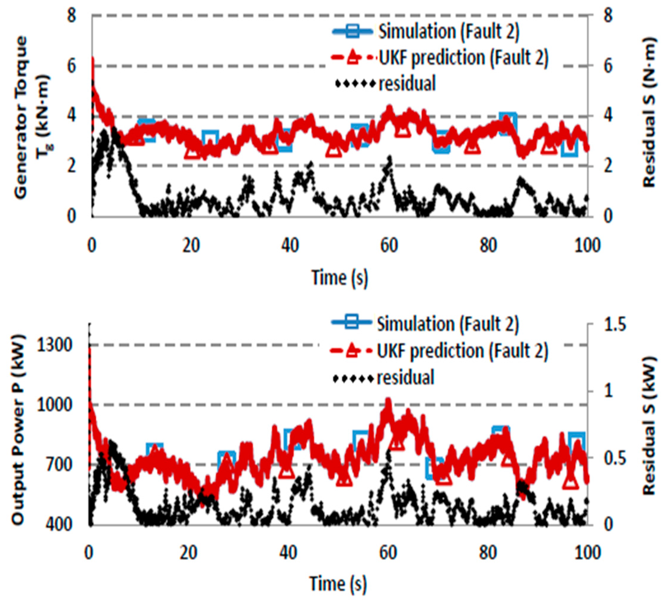
3.1. Diagnosis of Faults 1 and 2

The input wind speed varies between 9.5 and 10.5 m/s randomly. The results obtained by system process simulation for a WT in health, with Fault 1 and with Fault 2 are shown in Figure 3. Similar increasing trend of gearbox temperature-rise for a WT with Faults 1 and 2 are observed, which indicates difficulties of accurate fault identification by using signal trending analysis approaches such as data driven fault detection methods. For a WT with Fault 1, once gearbox transmission efficiency decreases the amount of energy dissipated increases. With Fault 2, due to the decrease of the flow rate of the lubrication oil, the energy dissipated by the lubrication oil reduced. Both failures could cause temperature rise of the WT lubrication oil. When the reduction amount of energy dissipated by the lubrication oil is similar to reduction amount of energy dissipated due to transmission efficiency reduction, the temperature rise of the two cases are similar. In fact, with the parameters set as above, these two types of energy amount are similar. Therefore, similar temperature rises are observed for the two failures.

The gearbox temperature-rise $\Delta T$ for a healthy WT is obtained from the UKF model with the same wind speed as input. Good agreement between UKF prediction and the simulation result are shown in Figure 4. It proves the validity of developed UKF model, which is capable to track the performance features of a healthy wind turbine.

Figure 5 shows the comparison between UKF predicted and simulation results of a WT with Fault 1. The comparisons are made between the performance parameters including gearbox temperature-rise (ΔT), rotor rotational speed (ω_r), generator torque (T_g) and power output (P). Gearbox temperature-rise predicted by UKF model is less than the simulation results, and their difference fluctuates between 5.4 and 6.9 K. By analyzing the WT process simulation model it is found that the output mechanical torque of a faulty gearbox decreases with the reduction of transmission efficiency due to the gear fatigue and wear. The reduction of mechanical torque subsequently causes controller to adjust the stator voltage of the generator to ensure stability of the system. This is proved by the UKF predicted reduced generator torque and output power as shown in Figure 5. Therefore, increase of rotor rotational speed is obtained. The model developed in UKF is to predict the system expected performance by considering a healthy WT. That is, the UKF model estimates a WT gearbox temperature rise with a varied stator voltage obtained from the WT system process that is actually under faulty situations. Therefore, the temperature-rise obtained by UKF method deviates from the simulation results under the same input condition. In addition, the UKF prediction of the ΔT, ω_r, T_g and P are dependent on results in the previous time slot, which results in cumulative enlargement of residual S as observed from Figure 5.

Figure 6 shows the UKF predicted gearbox temperature-rise is less than the simulation results under Fault 2 condition. The residual varies between 5.4 and 6.8 K consistently in time domain. By analyzing the mechanism of Fault 2 it is found that gearbox transmission efficiency is the same as healthy situation, which indicates the same amount of energy loss for this case. It is due to the variation of oil flow rate that leads to temperature rise of the lubrication oil. Therefore, the stator voltage U maintains the same as the value under healthy situation, which result in the same temperature rise predicted by UKF model as healthy situation. Due to the lubrication oil leakage, the actual WT gearbox temperature-rise increases, which is simulated by system process simulation by changing oil flow rate. The comparison between UKF result and the simulation result actually shows the comparison between WT system output under healthy and faulty situations. Less fluctuation of residual between UKF prediction and simulation results is observed for this case. However, as the gearbox transmission efficiency is the same as healthy situation the main energy transmission process is unaffected and then the expected rotor speed, torque and output power are the same as actually output. Therefore, good agreements between UKF model output and simulation results are observed.

Due to different influence of Faults 1 and 2 to performance parameters of a wind power system different rotor speed, generator torque, output power and gearbox temperature-rise predicted by UKF model are observed for Faults 1 and 2. The different behaviors of predicted results and tendency of residuals can be regarded as the feature of faults detection and identification.

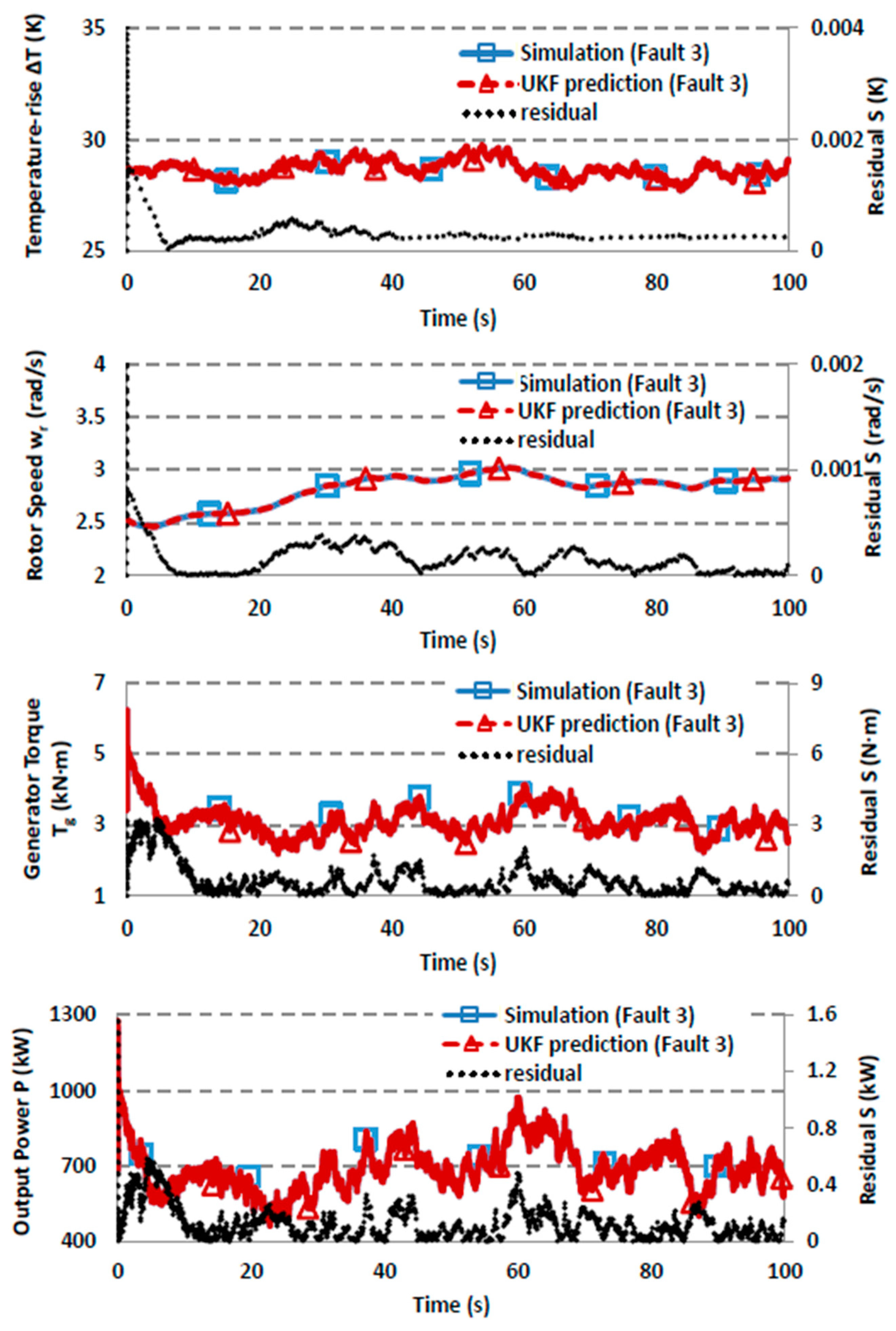
3.2. Diagnosis of Faults 1 and 3

To investigate UKF model performance for Fault 3 detection, the same random wind speed shown in Figure 3 is used. The simulated rotor rotational speed ω_r, electromagnetic torque T_g, output power P and gearbox temperature-rise ΔT of a WT under healthy situation and with Faults 1 and 3 are obtained and compared in Figure 7. It shows that the gearbox temperature-rise of a WT with Fault 1 is higher and that of a WT with Fault 3 is a little lower than a healthy one. The simulated generator torque and power of a WT with Faults 1 and 3 decrease with a similar trend. For a WT under speed control mode, the generator speed is controlled to ensure maximum power point tracking. When a WT has reduced gearbox efficiency (Fault 1), the energy is transmitted to the generator decrease. In order to maintain the same rotational speed for maximum power point tracking, the generator generates a reduced reversion torque and then lower output power. Therefore, a reduced generator torque and output power is observed for a WT under this failure mode. Similarly, when a wind turbine has a fixed (larger than normal situation) pitch angle and operates under rate wind speed range, the reduced energy extracted from wind speed results in reduced energy being transmitted to the generator. Then a reduced torque and output power is generated from the generator. The simulation results show the similar variation of the three outputs of Faults 1 and 3 in Figure 7, which also indicates challenge of fault identification of these two failure modes.

The cascaded UKF model is used to estimate ω_r, T_g and P of a WT with Fault 3. With the same wind speed as inputs, the comparison results of prediction and simulation are shown in Figure 8.

Figure 8 shows the comparison result between UKF model estimation and simulation. The predicted ω_r, T_g, P and ΔT from UKF is almost the same as the simulation result. It proves that with the faulty pitch angle, the UKF model is adaptive to the system. By analyzing the definition of the controlled vector for UKF model, it is found that pitch angle is one of the controlled vectors for the first UKF model and stator voltage is one of the controlled vectors of the second UKF model. UKF model exhibits different response for the varied pitch angle and the stator voltage. Different estimation output from UKF model under Fault 1 and Fault 3 conditions indicate different sensitivity of designed cascade UKF to different failure mode.

3.3. Discussion

The different mechanisms of Faults 1–3 cause the differences of the UKF estimated results for the failures. It can be regarded as effective fault features for fault diagnosis. Wind turbine is a complex nonlinear system with uncertain input. Its different failure modes may lead to similar fault features that cause challenge of fault diagnosis. By a proper design, the UKF model is proved to be effective in fault identification for different failure modes. Proper state space vector, control vectors should be defined for the UKF model. This is closely related to its fault detection sensitivity and then determines its effectiveness. For the three failure modes, which are Faults 1, 2 and 3, the systematic parameters that are changed due to failures, UKF model state space vectors and control vectors, the performances being monitored, residual variation tendencies are summarized and compared in

Table 2. System simulation and UKF model input and output parameters summary.

Fault Cases	System Process Simulation	Cascaded UKF Model
	System Parameters Variation	State Space Vector and Control Vectors	Monitoring Performances	Residual Tendencies
Fault 1	Ƞ ↓	UKF1: [ωr, ΔT]T, [v,β]T UKF2: Tg, [ωg, U]T	ΔT, ωr, Tg, P	S(ΔT) ↑, S(ωr) ↑, S(Tg) ↑, S(P) ↑
Fault 2	q ↓		ΔT, ωr, Tg, P	S(ΔT) ↑, S(ωr)~0, S(Tg)~0, S(P)~0
Fault 3	β (=45°)		ΔT, ωr, Tg, P	S(ΔT)~0, S(ωr)~0, S(Tg)~0, S(P)~0

.

(i)

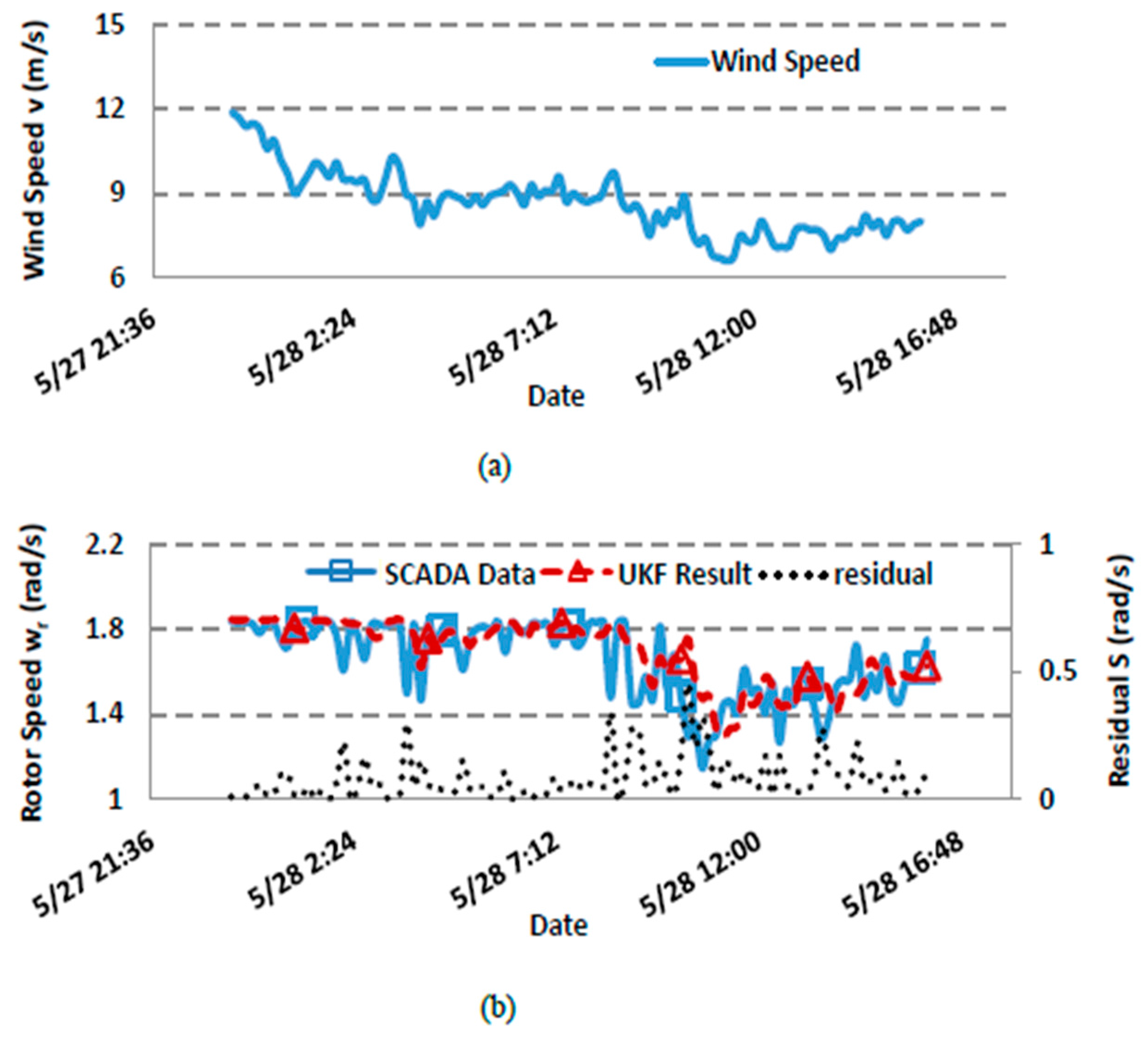
Fault 1 is representing such types of failures: due to a certain subcomponent (the gearbox in this case) degradation, local parameter (transmission efficiency) variation of the subcomponents causes WT different dynamic response. The control system changes certain process parameters (T_g and ω_r in this case) to adapt to the varied local parameters, and then to maintain a stable system according to control strategy. Analyzing residuals tendency of rotor speed, generator torque, output power and oil temperature-rise between simulated and UKF predicted results can identify Fault 1 from Faults 2 and 3.

(ii)

Fault 2 is presenting such types of failures: As not all subcomponents degradation will actively lead to WT different dynamic response, some failures only affect system performance. Assuming gearbox oil leakage had neglected effects on gearbox heat dissipation and only causes the portion of energy loss through oil to decrease. Unaffected system process parameters (T_g and U) are the input of UKF model. It makes UKF prediction the same as WT output under healthy condition. The actual WT output with fault compared to UKF model (healthy situation) shows consistent temperature rise residual. In this case, UKF model is designed for less sensitive to Fault 2 comparing to Fault 1. However, the different fault signatures can be defined for the two failures identification.

(iii)

Fault 3 is presenting such types of failures: key control parameters (pitch angle) of the system are varied due to components (pitch system) failure which directly changes the system response. With the UKF model defined with such parameters as an input controlled vector, the UKF model shows good adaptability for such varied input parameters. It delivers similar estimation output as the WT actually output under faulty condition. A proper UKF model can be re-defined in order to detect these types of failures for example to add additional module to judge the rationality of the input parameters of UKF. Although the UKF designed exhibits lower sensitivity to Fault 3, but Fault 1 can be easily identified from it.

The comparison above shows that by properly defining the state space vector (monitoring parameters) and control vector (key process parameters that is affected), UKF model is capable to deliver estimated value for the performance. Comparing simulated results and UKF predicted results and by analyzing their residual tendencies it is able to identify different failure modes. The UKF method exhibits different adaptability and sensitivity to failures and shows advances on certain failure mode detection.

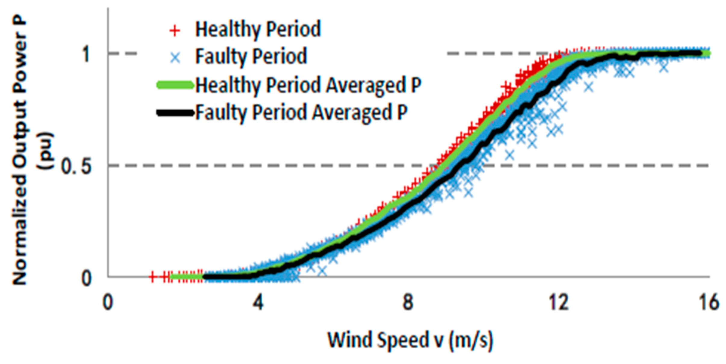
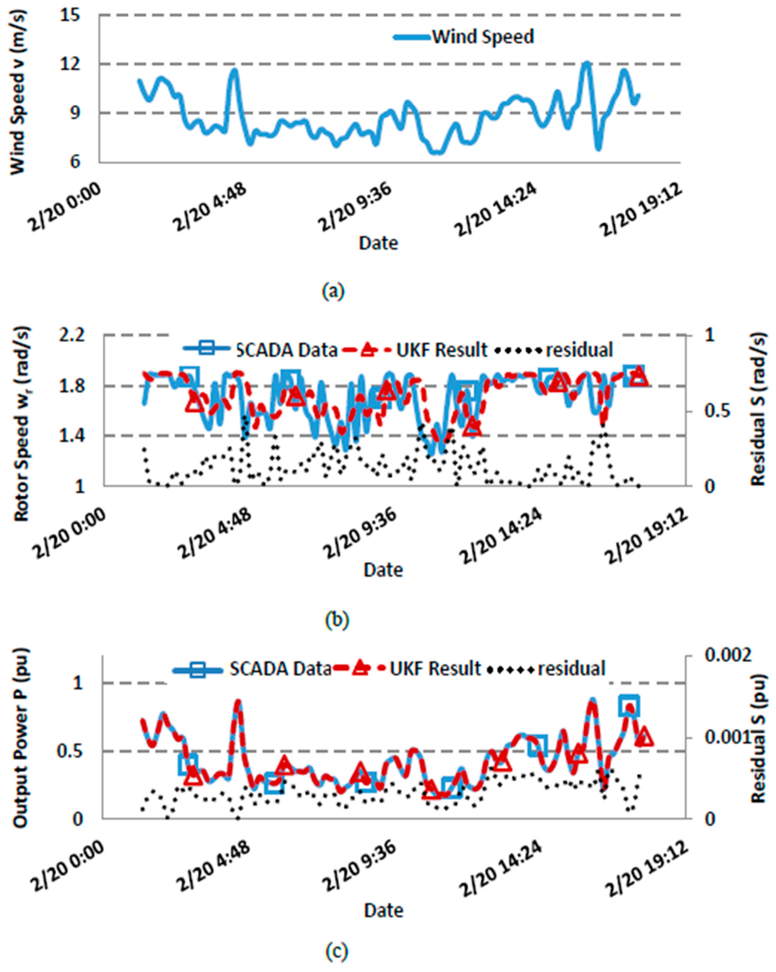
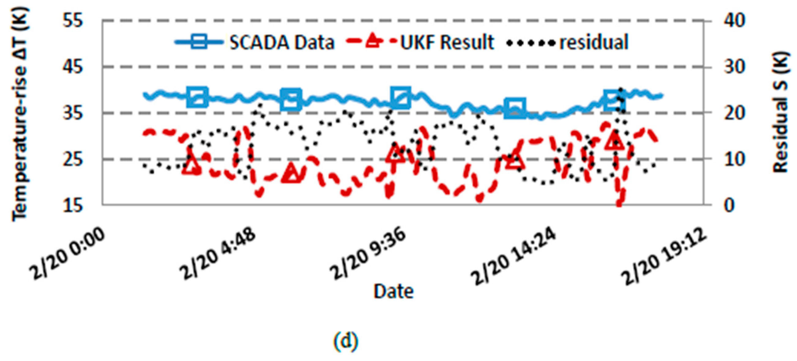
4. SCADA Data Analysis

To prove UKF model’s online fault detection feasibility, SCADA data from a WT with gearbox failure is used to investigate its fault detection capability. This WT is about 1.5–2 MW with the same configuration as discussed in Section 2. The date of the WT gearbox being replaced was recorded in March 2007. The data that is collected before the WT gearbox failure are divided into two periods. Each period contains the WT SCADA data for subsequent three months until WT failed. Therefore there are 6 months of data in total. Figure 9 shows the power curve of this WT for the two periods by assuming that the earlier three months data represents a healthy wind turbine performance.

The scattered plots in Figure 9 show the original SCADA data recorded and the lines are averaged SCADA output power under the same wind speeds for the two periods. It shows that WT’s output power of three months before failure deviates from healthy situation. Considering that the data recorded in the SCADA system is ten minute averaged values, there is no high sampling rate signals of control voltage U. Therefore, the state, input and measurement output are designed as Equation (23) to match the sampling rate of SCADA data.

$$\begin{array}{c}X={[{\mathsf{\omega }}_r,\Delta T]}^T\\ u={[v,T_g,\mathsf{\beta }]}^T\\ Y=P=N{\mathsf{\omega }}_r{T}_g\end{array}$$

(23)

Partial SCADA data in May 2006 and February 2007 are analysed with UKF method respectively, shown as Figure 10 and Figure 11.

The UKF method is used to estimate the output performance of a WT with input data recorded in SCADA system. Comparing Figure 10 and Figure 11 shows that although the fluctuation of rotor speed ω_r and output power P residuals were becoming larger in February 2007 than in May 2006, their differences between SCADA data and UKF prediction results are unobvious in consideration of the influences of wind speed, noise and average process of SCADA system. Therefore, rotor speed and output power may not be effective fault diagnosis parameters. While the magnitude of gearbox temperature-rise ΔT in Figure 11 is completely different from that in Figure 10. The temperature-rise in SCADA data a month before maintenance is higher than UKF prediction which is estimated as a healthy WT. The residual of temperature-rise in February 2007 is larger than in May 2006 obviously and it reached 10 K to 20 K. The result above can be used as the basis of WT gearbox fault diagnosis. It proves the effectiveness of UKF in fault diagnosis of WT with SCADA data.

5. Conclusions

This paper represents a procedure to develop physical-model-based cascaded unscented Kalman filter model for wind turbine fault detection. By analyzing the failure mechanism of the three different types of failures, a cascaded unscented Kalman filter model is designed and its fault detectabilities for the three failures are compared. Residuals behaviors between predicted results by unscented Kalman filter model and actual output (simulation process model) under the same input condition are analyzed for the three failures. It proves the applicability of the unscented Kalman filter method on wind turbine fault diagnosis. The result shows that due to wind turbine’s nonlinear characteristics and strong coupling between wind turbine subcomponents different failure modes have different effects to the WT process parameters. The designed unscented Kalman filter therefore shows different sensitivity to the failures. Properly defining state space vector (monitoring parameters) and control vector (key process parameters that is affected) for different failures are crucial for effective unscented Kalman filter model development.

In this paper, a new method of wind turbine fault diagnosis with SCADA data has been proposed. The simulation results show that model-based unscented Kalman filter method in this paper offers an effective means for detection of multiple faults in wind power system. The proposed method is able to make different responses to the SCADA data of wind turbines in health and fault, which shows its applicability to the online fault diagnosis of wind turbine. It gives successful examples and useful hints for future research that aiming at developing accurate wind turbine fault detection algorithms by designing proper input parameters of the algorithm. Extended research may also need to be performed to improve the fault detection robustness by defining a proper threshold for different failures, which not only depends on the failure model but also depends on the fault states. After all, the method proposed is useful for wind turbine condition monitoring system that is a core for improving wind turbines reliability and constructing scientific operational system of the wind farm.

References

- Yang, W.; Tavner, P.J.; Crabtree, C.J.; Feng, Y.; Qiu, Y. Wind turbine condition monitoring: Technical and commercial challenges. Wind Energy 2014, 17, 673–693. [Google Scholar] [CrossRef] [Green Version]
- Márquez, F.P.; Tobias, A.M.; Pérez, J.M.; Papaelias, M. Condition monitoring of wind turbines: Techniques and methods. Renew. Energy 2012, 46, 169–178. [Google Scholar] [CrossRef]
- Lu, B.; Li, Y.; Wu, X.; Yang, Z. A review of recent advances in wind turbine condition monitoring and fault diagnosis. In Proceedings of the IEEE Power Electronics and Machines in Wind Applications 2009, Lincoln, NE, USA, 24–26 June 2009.
- Qiu, Y.; Feng, Y.; Tavner, P.; Richardson, P.; Erdos, G.; Chen, B. Wind turbine SCADA alarm analysis for improving reliability. Wind Energy 2012, 15, 951–966. [Google Scholar] [CrossRef]
- Feng, Y.; Qiu, Y.; Crabtree, C.J.; Long, H.; Tavner, P.J. Monitoring wind turbine gearbox. Wind Energy 2013, 16, 728–740. [Google Scholar] [CrossRef]
- Kim, K.; Parthasarathy, G.; Uluyol, O.; Foslien, W.; Sheng, S.; Fleming, P. Use of SCADA Data for failure detection in wind turbines. In Proceedings of the 2011 Energy Sustainability Conference and Fuel Cell Conference, Washington, DC, USA, 7–10 August 2011.
- Zaher, A.S.; McArthur, S.D.; Infield, D.G.; Patel, Y. Online Wind Turbine Fault Detection through Automated SCADA Data Analysis. Wind Energy 2009, 12, 574–593. [Google Scholar] [CrossRef]
- Qiao, W.; Lu, D. A Survey on Wind Turbine Condition Monitoring and Fault Diagnosis—Part II: Signals and Signal Processing Methods. IEEE Trans. Ind. Electron. 2015, 62, 6536–6545. [Google Scholar] [CrossRef]
- Yang, W.; Court, R.; Jiang, J. Wind turbine condition monitoring by the approach of SCADA data analysis. Renew. Energy 2013, 53, 365–376. [Google Scholar] [CrossRef]
- Badihi, H.; Zhang, Y.; Hong, H. Wind Turbine Fault Diagnosis and Fault-Tolerant Torque Load Control against Actuator Faults. IEEE Trans. Control Syst. Technol. 2015, 23, 1351–1372. [Google Scholar] [CrossRef]
- Odgaard, P.F.; Stoustrup, J. Gear-box fault detection using time-frequency based methods. Annu. Rev. Control 2015, 40, 50–58. [Google Scholar] [CrossRef]
- Venkatasubramanian, V.; Rengaswamy, R.; Yin, K.; Kavuri, S.N. A review of process fault detection and diagnosis: Part I: Quantitative model based methods. Comput. Chem. Eng. 2003, 27, 293–311. [Google Scholar] [CrossRef]
- Wilkinson, M.; Darnell, B.; Van Delft, T.; Harman, K. Comparison of methods for wind turbine condition monitoring with SCADA data. IET Renew. Power Gener. 2014, 8, 390–397. [Google Scholar] [CrossRef]
- Cross, P.; Ma, X. Nonlinear system identification for model-based condition monitoring of wind turbines. Renew. Energy 2014, 71, 166–175. [Google Scholar] [CrossRef] [Green Version]
- Dey, S.; Pisu, P.; Ayalew, B. A comparative study of three fault diagnosis schemes for wind turbines. IEEE Trans. Control Syst. Technol. 2015, 23, 1853–1868. [Google Scholar] [CrossRef]
- Qiu, Y.; Feng, Y.; Sun, J.; Zhang, W.; Infield, D. Applying thermophysics for wind turbine drivetrain fault diagnosis using SCADA data. IET Renew. Power Gener. 2016, 10, 661–668. [Google Scholar] [CrossRef] [Green Version]
- Qiu, Y.; Zhang, W.; Cao, M.; Feng, Y.; Infield, D. An electro-thermal analysis of a variable-speed doubly-fed induction generator in a wind turbine. Energies 2015, 8, 3386–3402. [Google Scholar] [CrossRef] [Green Version]
- Mengnan, C.; Yingning, Q.; Yanhui, F.; Hao, W.; Infield, D. Wind turbine fault diagnosis based on unscented Kalman Filter. In Proceedings of the International Conference on Renewable Power Generation (RPG 2015), Beijing, China, 17–18 October 2015.
- Julier, S.J.; Uhlmann, J.K. Unscented filtering and nonlinear estimation. Proc. IEEE 2004, 92, 401–422. [Google Scholar] [CrossRef]
- Gonçalves, D.E.; Fernandes, C.M.; Martins, R.C.; Seabra, J.H. Torque loss in a gearbox lubricated with wind turbine gear oils. Lubr. Sci. 2013, 25, 297–311. [Google Scholar] [CrossRef]
- Bergman, T.L.; Incropera, F.P.; DeWitt, D.P.; Lavine, A.S. Fundamentals of Heat and Mass Transfer, 6th ed.; John Wiley & Sons: New York, NY, USA, 2006; p. 100. [Google Scholar]
- Simon, D. Optimal State Estimation: Kalman, H Infinity, and Nonlinear Approaches; Wiley-Interscience: New York, NY, USA, 2006. [Google Scholar]
- Mirzaee, A.; Salahshoor, K. Fault diagnosis and accommodation of nonlinear systems based on multiple-model adaptive unscented Kalman Filter and switched MPC and H-infinity loop-shaping controller. J. Process Control 2012, 22, 626–634. [Google Scholar] [CrossRef]