
Spatial and Temporal Traffic Variation in Core Networks: Impact on Energy Saving and Devices Lifetime †


Abstract
:1. Introduction
2. Related Work
3. Traffic Model
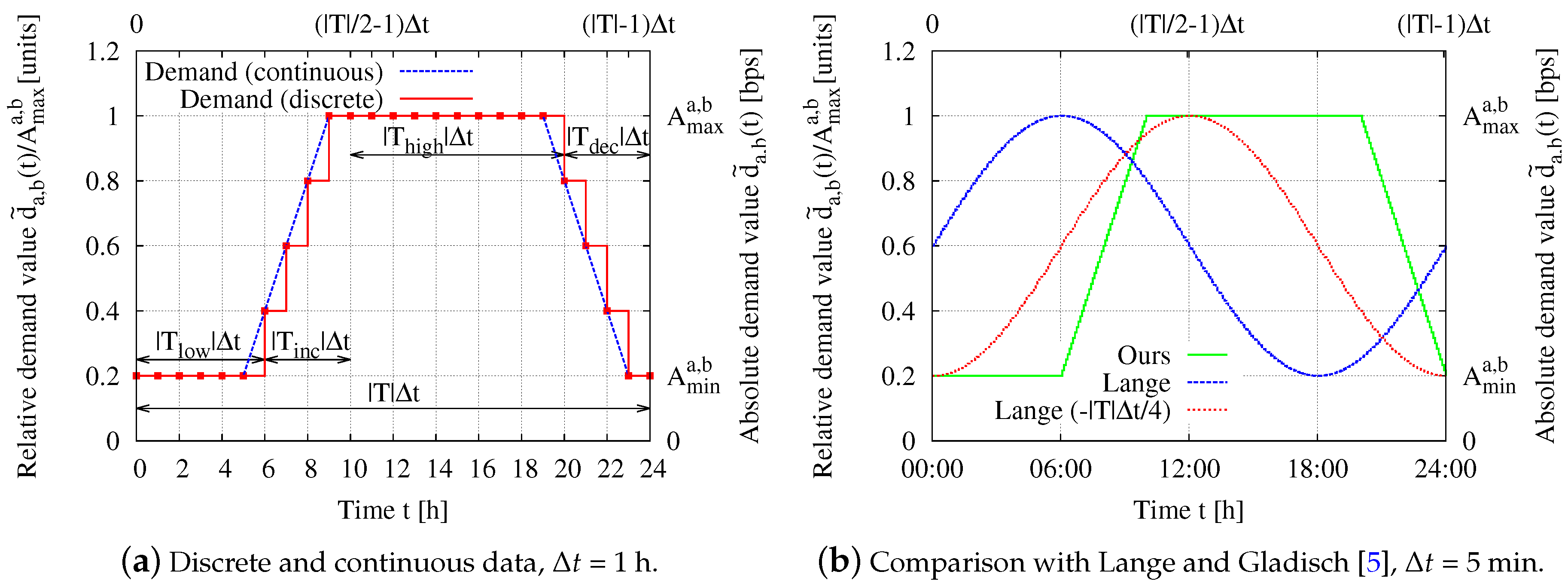
3.1. Temporal Traffic Variation
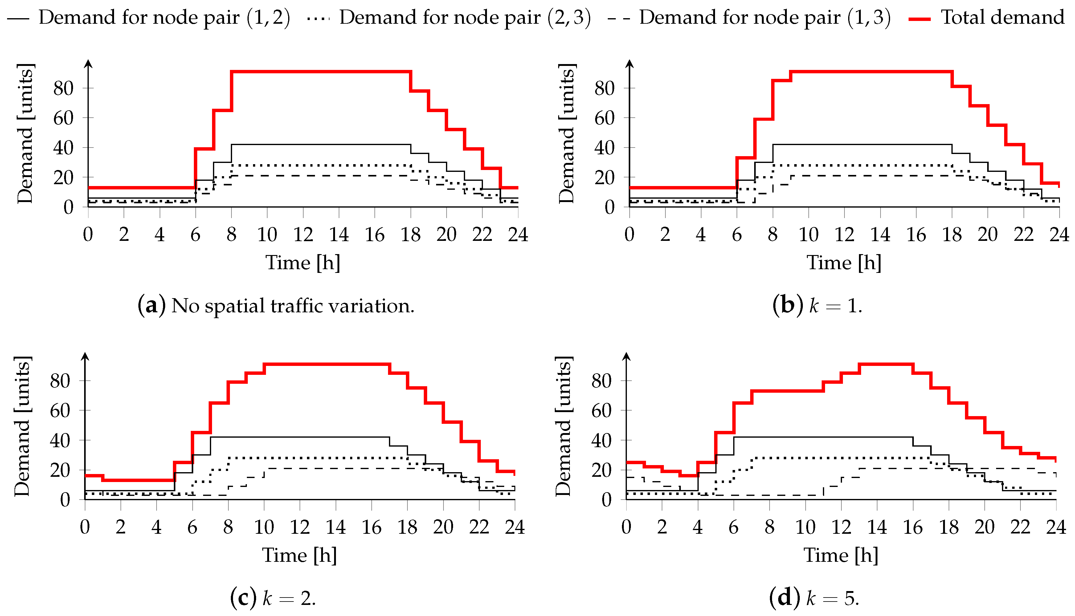
3.2. Spatial Traffic Variation
4. Network Model
4.1. Assumptions
4.2. Network Design
4.3. Network Operation
5. Evaluation Scenario
5.1. Traffic and Network
5.2. CapEx and Power
5.3. Evaluation Metrics
5.3.1. Energy Consumption
5.3.2. Normalized Lifetime
5.3.3. Network Profitability
6. Results
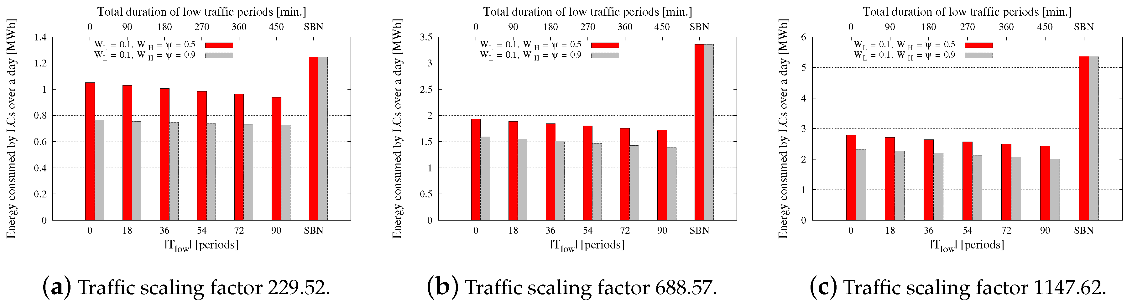
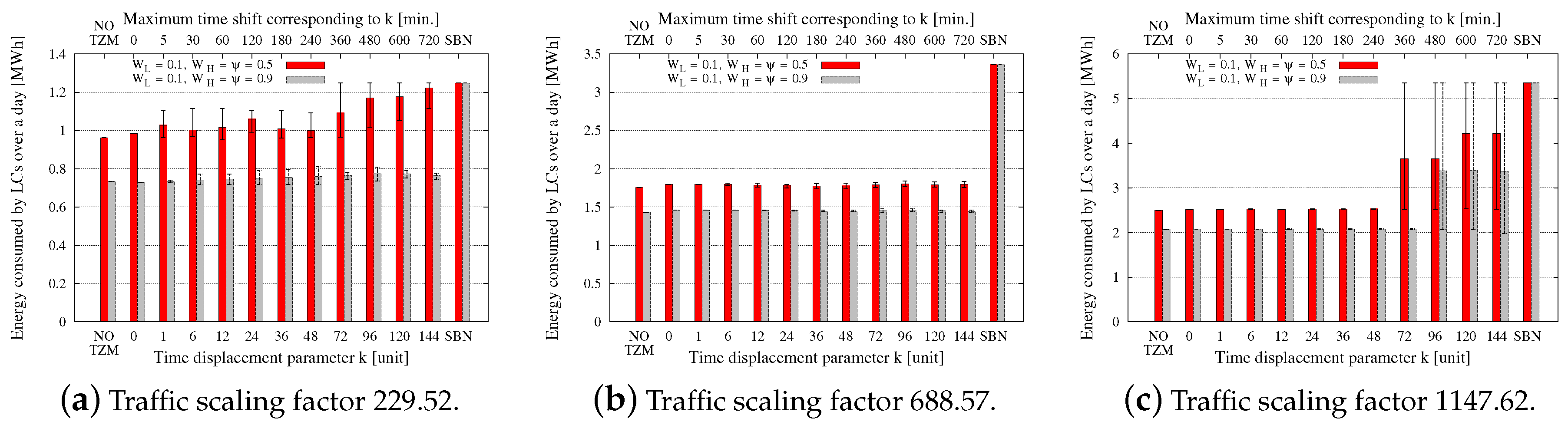
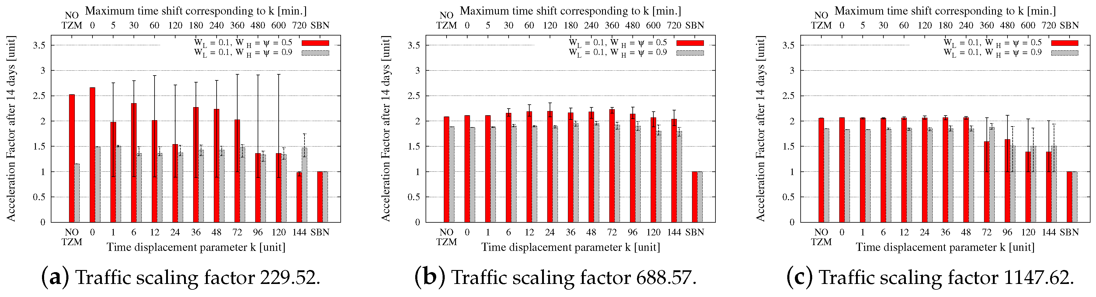
6.1. Influence of Temporal Traffic Variation
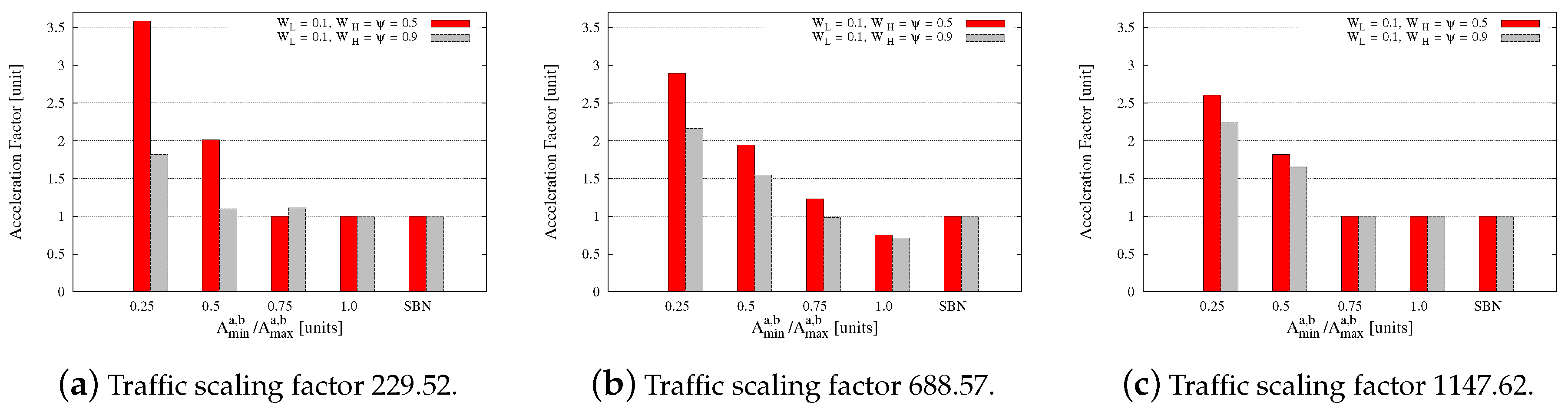
6.2. Influence of Spatial Traffic Variation
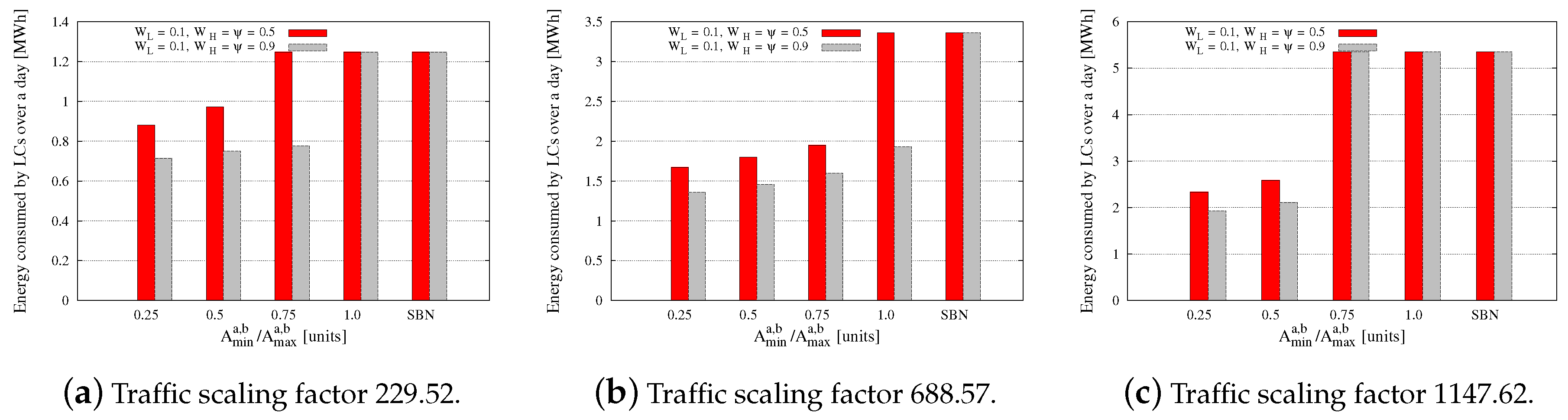
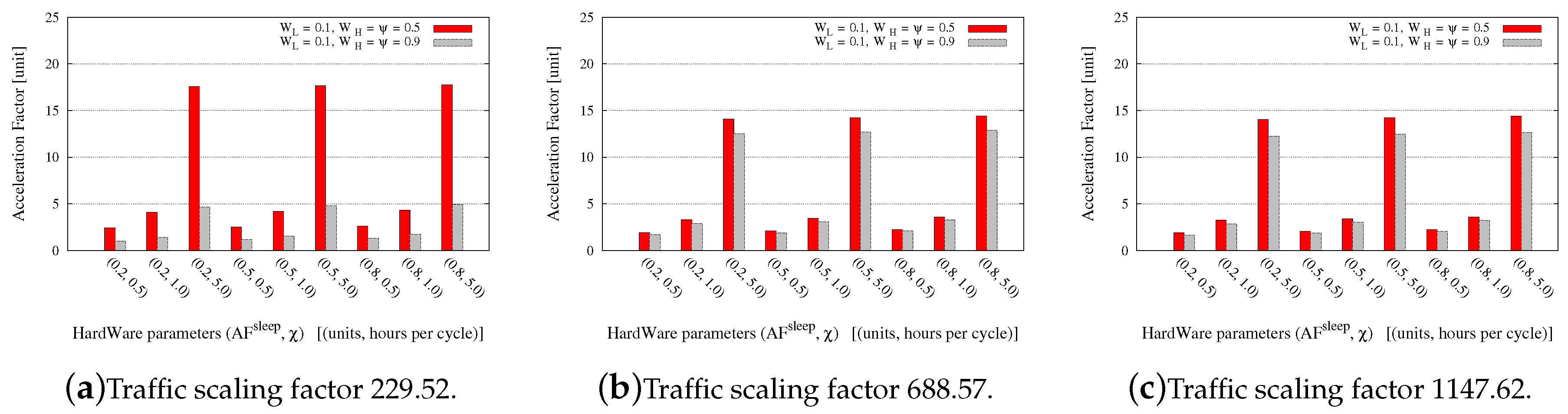
6.3. Influence of HW Parameters
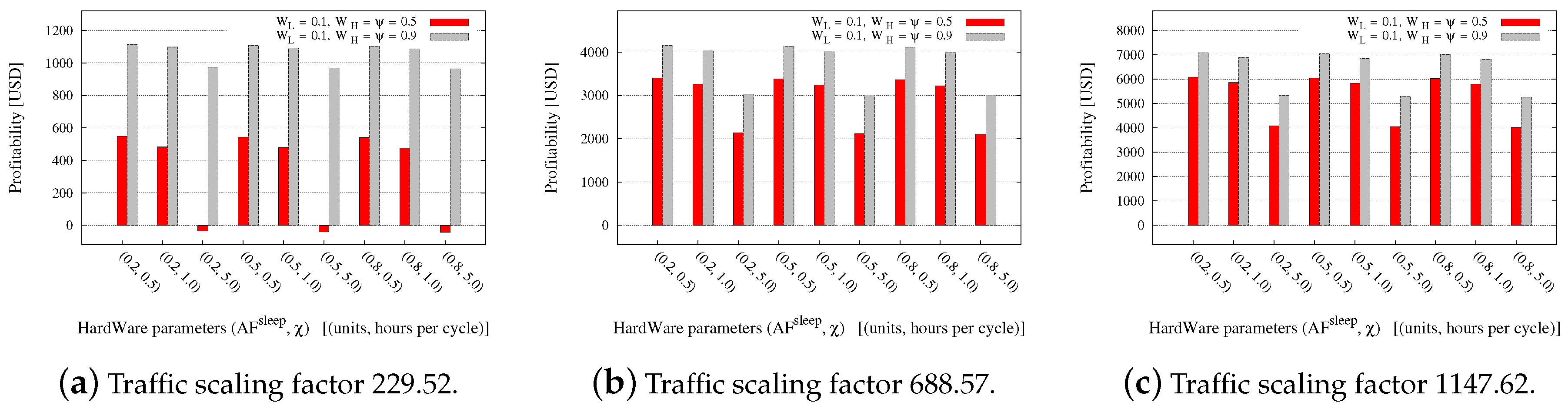
6.4. Evaluation of Network Profitability
7. Conclusions
Acknowledgments
Author Contributions
Conflicts of Interest
Abbreviations
| AF | Acceleration Factor |
| AM | Active Mode |
| CapEx | Capital Expenditure |
| CPU | Central Processing Unit |
| DGE | Dynamic Gain Equalizer |
| EWA | Energy Watermark Algorithm |
| FR | Failure Rate |
| GMT | Greenwich Mean Time |
| HW | HardWare |
| IP | Internet Protocol |
| LC | Line Card |
| MILP | Mixed-Integer Linear Programming |
| MTTR | Mean Time To Repair |
| OLA | Optical Line Amplifier |
| OpEx | Operational Expenditure |
| OSPF | Open Shortest Path First |
| OXC | Optical Cross-Connect |
| QoS | Quality of Service |
| RAM | Random-Access Memory |
| SBN | Static Base Network |
| SM | Sleep Mode |
| SVM | Spatial Variation Matrix |
| TZM | Time Zone Matrix |
| WDM | Wavelength Division Multiplexing |
Appendix A

| Minimize cost |
| subject to |
| using variables |
| Symbol | Description | |
|---|---|---|
| General and MILP | undirected physical supply network with set of nodes V and set of physical supply links | |
| undirected logical supply network with set of nodes V and set of logical supply links | ||
| C | capacity of a lightpath | |
| B | number of wavelengths per fiber | |
| P | set of all (undirected) paths through G on which capacity modules can be installed | |
| set of all paths from P where one of the end nodes is | ||
| set of all paths from P whose end nodes are the end nodes of | ||
| set of all paths from P that traverse physical supply link | ||
| N | set of routers that can be installed in the network | |
| capacity of router | ||
| δ | maximum lightpath utilization, | |
| CapEx cost of installing an OXC | ||
| CapEx cost of installing router | ||
| CapEx cost of installing a lightpath with LC | ||
| CapEx cost of installing a fiber on physical supply link | ||
| EWA | threshold on the utilization of the last lightpath on a logical link to trigger attempts to release lightpaths, | |
| threshold on the utilization of the last lightpath on a logical link to trigger attempts to establish new lightpaths, | ||
| ψ | maximum utilization of the last lightpath on a logical link, | |
| number of LCs installed at node | ||
| Time and traffic | T | set of considered time periods in the proposed traffic model |
| set of time periods covered by traffic measurements | ||
| set of time periods with low traffic, | ||
| set of time periods with high traffic, | ||
| set of time periods with increasing traffic, | ||
| set of time periods with decreasing traffic, | ||
| length of each time period | ||
| length of each time period | ||
| maximum traffic demand value for the node pair in the proposed traffic model | ||
| minimum traffic demand value for the node pair in the proposed traffic model | ||
| , | traffic demand between the ordered node pair during time period without (with) spatial variation (Equations (5) and (1)) | |
| maximum traffic demand between the ordered node pair (Equation (8)) | ||
| , | maximum emanating (ending) traffic demand at node (Equation (A11)) | |
| measured traffic demand between the ordered node pair during time period | ||
| s | scaling factor to account for increased traffic demands with respect to the time when the original traffic data was captured | |
| Θ | TZM with denoting an element of the TZM Θ, | |
| Γ | SVM with denoting an element of the SVM Γ, | |
| k | time displacement parameter, | |
| number of time periods by which the demand between nodes is shifted temporally due to spatial traffic variation | ||
| Evaluation | power of a LCs (W) | |
| ratio between the failure rates of an LCs dynamically switched between sleep and active modes and of the LCs kept active | ||
| χ | weight for the frequency of the active-sleep-active mode cycles of a LCs (h/cycle) | |
| Mean Time To Repair (MTTR) of a LCs (h) | ||
| Failure Rate (FR) of a LCs (failure/h) | ||
| cost of energy (USD/Wh) | ||
| hourly rate of a reparation crew member (USD/h/period) |
| MILP | —whether or not the traffic demand from node to traverses the logical link in the direction from to | |
| —whether or not the logical link from to is installed (i.e., traversed by any traffic in any direction) | ||
| —node potential for node and node , such that is a lower bound for the shortest path from to using only installed logical links | ||
| —number of lightpaths established on path | ||
| —whether or not router module is installed at node ; is a variable for SBN design and a parameter for evaluations of energy saving during network operation | ||
| —number of fibers installed on physical link ; is a variable for SBN design and a parameter for evaluations of energy saving during network operation | ||
| total energy consumed by LCs in the SBN (not using SM) after all (Wh) | ||
| EWA | —whether or not the traffic demand from node to traverses the logical link in the direction from to in time period | |
| —number of lightpaths forming logical link in time period | ||
| , —number of LCs active at node in time period | ||
| Evaluation | AF of the k-th LCs at node at time | |
| time spent in sleep mode by the k-th LCs at node up to time | ||
| number of SM-AM-SM cycles of the k-th LCs at node up to time | ||
| total energy consumed by LCs using SM and EWA after all (Wh) | ||
| average AF over all LCs in the network after all (unit) | ||
| total profitability after all (USD) |
References
- Zhang, Y.; Chowdhury, P.; Tornatore, M.; Mukherjee, B. Energy Efficiency in Telecom Optical Networks. IEEE Commun. Surv. Tutor. 2010, 12, 441–458. [Google Scholar] [CrossRef]
- Idzikowski, F.; Chiaraviglio, L.; Cianfrani, A.; López Vizcaíno, J.; Polverini, M.; Ye, Y. A Survey on Energy-Aware Design and Operation of Core Networks. IEEE Commun. Surv. Tutor. 2016, 18, 1453–1499. [Google Scholar] [CrossRef]
- Chiaraviglio, L.; Wiatr, P.; Monti, P.; Chen, J.; Lorincz, J.; Idzikowski, F.; Listanti, M.; Wosinska, L. Is green networking beneficial in terms of device lifetime? IEEE Commun. Mag. 2015, 53, 232–240. [Google Scholar] [CrossRef]
- Lange, C.; Gladisch, A. Energy efficiency limits of load adaptive networks. In Proceedings of the 2010 Conference on Optical Fiber Communication (OFC), Collocated National Fiber Optic Engineers Conference, San Diego, CA, USA, 21–25 March 2010.
- Lange, C.; Gladisch, A. Limits of Energy Efficiency Improvements by Load-Adaptive Telecommunication Network Operation. In Proceedings of the 10th Conference of Telecommunication, Media and Internet Techno-Economics (CTTE), Berlin, Germany, 16–18 May 2011.
- Idzikowski, F.; Pfeuffer, F.; Werner, A.; Chiaraviglio, L. Impact of Spatial Traffic Variation on Energy Savings and Devices Lifetime in Core Networks. In Proceedings of the 2016 IEEE 17th International Conference on High Performance Switching and Routing (HPSR), Yokohama, Japan, 14–17 June 2016.
- Almeida, S.; Queijo, J.; Correia, L.M. Spatial and temporal traffic distribution models for GSM. In Proceedings of the 1999 Fall IEEE VTS 50th Vehicular Technology Conference, Amsterdam, The Netherlands, 19–22 September 1999.
- Lee, D.; Zhou, S.; Zhong, X.; Niu, Z.; Zhou, X.; Zhang, H. Spatial modeling of the traffic density in cellular networks. IEEE Wirel. Commun. 2014, 21, 80–88. [Google Scholar] [CrossRef]
- Wu, Y.; Min, G.; Li, K.; Javadi, B. Modeling and Analysis of Communication Networks in Multicluster Systems under Spatio-Temporal Bursty Traffic. IEEE Trans. Parallel Distrib. Syst. 2012, 23, 902–912. [Google Scholar] [CrossRef]
- Coiro, A.; Iervini, F.; Listanti, M. Distributed and Adaptive Interface Switch Off for Internet Energy Saving. In Proceedings of the 20th International Conference on Computer Communications and Networks (ICCCN), New Delhi, India, 31 July–4 August 2011.
- Coiro, A.; Listanti, M.; Valenti, A. Impact of Energy-Aware Topology Design and Adaptive Routing at Different Layers in IP over WDM networks. In Proceedings of the XVth International Telecommunications Network Strategy and Planning Symposium (NETWORKS), Rome, Italy, 15–18 October 2012.
- Coiro, A.; Listanti, M.; Valenti, A.; Matera, F. Energy-aware traffic engineering: A routing-based distributed solution for connection-oriented IP networks. Comput. Netw. 2013, 57, 2004–2020. [Google Scholar] [CrossRef]
- Chiaraviglio, L.; Mellia, M.; Neri, F. Energy-aware Backbone Networks: A Case Study. In Proceedings of the 2009 IEEE International Conference on Communications Workshops, Dresden, Germany, 14–18 June 2009.
- Scharf, J. Efficiency Analysis of Distributed Dynamic Optical Bypassing Heuristics. In Proceedings of the 2012 IEEE International Conference on Communications (ICC), Ottawa, ON, Canada, 10–15 June 2012.
- Lui, Y.; Shen, G.; Shao, W. Optimal Port Grouping for Maximal Router Card Sleeping. In Proceedings of the 2012 Asia Communications and Photonics Conference (ACP), Guangzhou, China, 7–10 November 2012.
- Lui, Y.; Shen, G.; Bose, S.K. Energy-Efficient Opaque IP over WDM Networks with Survivability and Security Constraints. In Proceedings of the 2013 Asia Communications and Photonics Conference, Beijing, China, 12–15 November 2013.
- Lui, Y.; Shen, G.; Shao, W. Design for Energy-Efficient IP Over WDM Networks With Joint Lightpath Bypass and Router-Card Sleeping Strategies. J. Opt. Commun. Netw. 2013, 5, 1122–1138. [Google Scholar] [CrossRef]
- Chiaraviglio, L.; Mellia, M.; Neri, F. Reducing Power Consumption in Backbone Networks. In Proceedings of the 2009 IEEE International Conference on Communications (ICC), Dresden, Germany, 14–18 June 2009.
- Bianzino, A.P.; Chaudet, C.; Moretti, S.; Rougier, J.L.; Chiaraviglio, L.; Le Rouzic, E. Enabling Sleep Mode in Backbone IP-Networks: A Criticality-Driven Tradeoff. In Proceedings of the 2012 IEEE International Conference on Communications, Ottawa, ON, Canada, 10–15 June 2012.
- Bianzino, A.P.; Chiaraviglio, L.; Mellia, M. GRiDA: A Green Distributed Algorithm for Backbone Networks. In Proceedings of the 2011 IEEE Online Conference on Green Communications (GreenCom), New York, NY, USA, 26–29 September 2011.
- Bianzino, A.P.; Chiaraviglio, L.; Mellia, M.; Rougier, J.L. GRiDA: GReen Distributed Algorithm for energy-efficient IP backbone networks. Comput. Netw. 2012, 56, 3219–3232. [Google Scholar] [CrossRef]
- Tego, E.; Idzikowski, F.; Chiaraviglio, L.; Coiro, A.; Matera, F. Facing the reality: Validation of energy saving mechanisms on a testbed. J. Electr. Comput. Eng. 2014, 2014, 1–11. [Google Scholar] [CrossRef]
- Dong, X.; El-Gorashi, T.; Elmirghani, J. Hybrid-power IP over WDM network. In Proceedings of the 2010 Seventh International Conference On Wireless And Optical Communications Networks (WOCN), Colombo, Sri Lanka, 6–8 September 2010.
- Dong, X.; El-Gorashi, T.; Elmirghani, J. IP over WDM Networks Employing Renewable Energy Sources. J. Lightwave Technol. 2011, 29, 3–14. [Google Scholar] [CrossRef]
- Dong, X.; El-Gorashi, T.; Elmirghani, J. Energy Efficient Optical Networks with Minimized Non-Renewable Power Consumption. J. Netw. 2012, 7, 821–831. [Google Scholar] [CrossRef]
- Dong, X.; El-Gorashi, T.; Elmirghani, J. Energy-Efficient IP over WDM Networks with Data Centres. In Proceedings of the 2011 13th International Conference on Transparent Optical Networks (ICTON), Stockholm, Sweden, 26–30 June 2011.
- Dong, X.; El-Gorashi, T.; Elmirghani, J. Green IP Over WDM Networks With Data Centers. J. Lightwave Technol. 2011, 29, 1861–1880. [Google Scholar] [CrossRef]
- Dong, X.; Lawey, A.; El-Gorashi, T.; Elmirghani, J. Energy-Efficient Core Networks. In Proceedings of the 2012 16th International Conference on Optical Network Design and Modeling (ONDM), Colchester, UK, 17–20 April 2012.
- Dong, X.; El-Gorashi, T.; Elmirghani, J. On the Energy Efficiency of Physical Topology Design for IP Over WDM Networks. J. Lightwave Technol. 2012, 30, 1931–1942. [Google Scholar] [CrossRef]
- Mukherjee, B. Optical WDM Networks; Springer: New York, NY, USA, 2006. [Google Scholar]
- Betker, A.; Gamrath, I.; Kosiankowski, D.; Lange, C.; Lehmann, H.; Pfeuffer, F.; Simon, F.; Werner, A. Comprehensive Topology and Traffic Model of a Nationwide Telecommunication Network. J. Opt. Commun. Netw. 2014, 6, 1038–1047. [Google Scholar] [CrossRef]
- Ahmad, A.; Bianco, A.; Bonetto, E.; Chiaraviglio, L.; Idzikowski, F. Energy-Aware Design of Multi-layer Core Networks. J. Opt. Commun. Netw. 2013, 5, A127–A143. [Google Scholar] [CrossRef]
- Bonetto, E.; Chiaraviglio, L.; Idzikowski, F.; Le Rouzic, E. Algorithms for the Multi-Period Power-Aware Logical Topology Design with Reconfiguration Costs. J. Opt. Commun. Netw. 2013, 5, 394–410. [Google Scholar] [CrossRef]
- Idzikowski, F.; Bonetto, E.; Chiaraviglio, L. EWA—An Adaptive Algorithm Using Watermarks for Energy Saving in IP-Over-WDM Networks; Technical Report TKN-12-002; Technische Universität Berlin: Berlin, Germany, 2012. [Google Scholar]
- Zhang, Y. 6 Months of Abilene Traffic Matrices. Available online: http://www.cs.utexas.edu/~yzhang/research/AbileneTM/ (accessed on 13 October 2016).
- Zuse Institut Berlin. Library of test instances for Survivable fixed telecommunication Network Design. Available online: http://sndlib.zib.de/home.action (accessed on 13 October 2016).
- Idzikowski, F.; Chiaraviglio, L.; Portoso, F. Optimal Design of Green Multi-layer Core Networks. In Proceedings of the 2012 Third International Conference on Future Energy Systems: Where Energy, Computing and Communication Meet (e-Energy), Madrid, Spain, 9–11 May 2012.
- Hülsermann, R.; Gunkel, M.; Meusburger, C.; Schupke, D.A. Cost Modeling and Evaluation of Capital Expenditures in Optical Multilayer Networks. J. Opt. Netw. 2008, 7, 814–833. [Google Scholar] [CrossRef]
- Van Heddeghem, W.; Idzikowski, F. Equipment Power Consumption in Optical Multilayer Networks—Source Data; Technical Report IBCN-12-001-01; Ghent University: Ghent, Belgium, 2012. [Google Scholar]
- Zhang, Y.; Tornatore, M.; Chowdhury, P.; Mukherjee, B. Energy optimization in IP-over-WDM networks. Opt. Switch. Netw 2011, 8, 171–180. [Google Scholar] [CrossRef]
- Arrhenius, S. Über die Reaktionsgeschwindigkeit Bei der Inversion von Rohrzucker Durch Säuren; Wilhelm Engelmann: Leipzig, Germany, 1889. [Google Scholar]
- Wiatr, P.; Chen, J.; Monti, P.; Wosinska, L. Energy Efficiency versus Reliability Performance in Optical Backbone Networks. J. Opt. Commun. Netw. 2015, 7, A482–A491. [Google Scholar] [CrossRef]
- European Commission. Energy Prices and Costs Report. Available online: http://ec.europa.eu/energy/sites/ener/files/documents/20140122_swd_prices.pdf (accessed on 13 October 2016).
- Cisco ONS 15454 Multiservice Transport Platform—MSTP. Available online: http://www.cisco.com/c/en/us/products/optical-networking/ons-15454-multiservice-transport-platform-mstp/index.html (accessed on 16 August 2016).
- Wiatr, P.; Chen, J.; Monti, P.; Wosinska, L. Energy saving in access networks: Gain or loss from the cost perspective? In Proceedings of the 2013 15th International Conference on Transparent Optical Networks (ICTON), Cartagena, Spain, 23–27 June 2013.
- IBM–ILOG. Cplex 12.6.0. Available online: http://www.ibm.com/software/commerce/optimization/cplex-optimizer/ (accessed on 13 October 2016).
- Pióro, M.; Medhi, D. Routing, Flow, and Capacity Design in Communication and Computer Networks; Morgan Kaufmann Publishers: San Mateo, CA, USA, 2004. [Google Scholar]


| Parameter(s) | Values | Corresponding Time Ranges (h) |
|---|---|---|
| - | ||
| 0–7.5 | ||
| 10.5–18 | ||
| 0–3.75 | ||
| 0–3.75 | ||
| k | 0–12 |
| , | , | ||||
|---|---|---|---|---|---|
| (Units) | (min) | (MWh) | (Units) | (MWh) | (Units) |
| 0 | 0 | 3780.00 | 0.81 | 2065.50 | 2.19 |
| 9 | 45 | 2516.58 | 2.11 | 2069.38 | 1.83 |
| 18 | 90 | 2502.71 | 2.07 | 2069.00 | 1.85 |
| 27 | 135 | 2496.38 | 2.06 | 2068.63 | 1.83 |
| 36 | 180 | 2497.25 | 2.06 | 2068.38 | 1.85 |
| 45 | 225 | 2498.50 | 2.06 | 2065.67 | 1.84 |
| SBN | 5352.00 | 1.00 | 5352.00 | 1.00 | |
© 2016 by the authors; licensee MDPI, Basel, Switzerland. This article is an open access article distributed under the terms and conditions of the Creative Commons Attribution (CC-BY) license (http://creativecommons.org/licenses/by/4.0/).
Share and Cite
Idzikowski, F.; Pfeuffer, F.; Werner, A.; Chiaraviglio, L. Spatial and Temporal Traffic Variation in Core Networks: Impact on Energy Saving and Devices Lifetime. Energies 2016, 9, 837. https://doi.org/10.3390/en9100837
Idzikowski F, Pfeuffer F, Werner A, Chiaraviglio L. Spatial and Temporal Traffic Variation in Core Networks: Impact on Energy Saving and Devices Lifetime. Energies. 2016; 9(10):837. https://doi.org/10.3390/en9100837
Chicago/Turabian StyleIdzikowski, Filip, Frank Pfeuffer, Axel Werner, and Luca Chiaraviglio. 2016. "Spatial and Temporal Traffic Variation in Core Networks: Impact on Energy Saving and Devices Lifetime" Energies 9, no. 10: 837. https://doi.org/10.3390/en9100837
APA StyleIdzikowski, F., Pfeuffer, F., Werner, A., & Chiaraviglio, L. (2016). Spatial and Temporal Traffic Variation in Core Networks: Impact on Energy Saving and Devices Lifetime. Energies, 9(10), 837. https://doi.org/10.3390/en9100837