Article

The Relationship between Residential Electricity Consumption and Income: A Piecewise Linear Model with Panel Data

1
School of Management and Economics, Beijing Institute of Technology, 5 Zhongguancun South Street, Haidian District, Beijing 100081, China
2
Center for Energy and Environmental Policy Research, Beijing Institute of Technology, 5 Zhongguancun South Street, Haidian District, Beijing 100081, China
3
Collaborative Innovation Center of Electric Vehicles in Beijing, 5 Zhongguancun South Street, Haidian District, Beijing 100081, China
4
Department of Natural Resources and the Environment, University of New Hampshire, 56 College Road, Durham, NH 03824, USA
*
Author to whom correspondence should be addressed.
Energies 2016, 9(10), 831; https://doi.org/10.3390/en9100831
Submission received: 11 August 2016 / Revised: 24 September 2016 / Accepted: 11 October 2016 / Published: 17 October 2016
(This article belongs to the Special Issue Energy Policy and Climate Change 2016)

Abstract

:
There are many uncertainties and risks in residential electricity consumption associated with economic development. Knowledge of the relationship between residential electricity consumption and its key determinant—income—is important to the sustainable development of the electric power industry. Using panel data from 30 provinces for the 1995–2012 period, this study investigates how residential electricity consumption changes as incomes increase in China. Previous studies typically used linear or quadratic double-logarithmic models imposing ex ante restrictions on the indistinct relationship between residential electricity consumption and income. Contrary to those models, we employed a reduced piecewise linear model that is self-adaptive and highly flexible and circumvents the problem of “prior restrictions”. Robust tests of different segment specifications and regression methods are performed to ensure the validity of the research. The results provide strong evidence that the income elasticity was approximately one, and it remained stable throughout the estimation period. The income threshold at which residential electricity consumption automatically remains stable or slows has not been reached. To ensure the sustainable development of the electric power industry, introducing higher energy efficiency standards for electrical appliances and improving income levels are vital. Government should also emphasize electricity conservation in the industrial sector rather than in residential sector.

1. Introduction

Electricity is one of the cleanest and most efficient terminal energies. Regardless of whether they are fossil fuels-based or renewable, most energies will finally convert into electricity. Therefore, electricity has become the preferred and dominant form of energy used in households in developed and fast developing countries, satisfying a varied range of needs from necessities to recreational and luxury consumption [1,2]. Therefore, the residential electricity consumption level and its proportion to total energy consumption are important benchmarks for measuring the extent of living modernization. During the past two decades, China has experienced rapid economic growth and an improvement of modern living standards, driving a soaring increase in residential energy consumption. The consumption level was 1006 billion kWh in 1995, and the figure climbed drastically to 6219 billion kWh in 2012 and is rising at a rate of 12.35%. The booming residential electricity consumption is also embodied in the ownership of household electrical appliances. As shown in Figure 1, the ownership of washing machines, refrigerators, televisions, air conditioners and other household appliances increased substantially both in China's urban and rural areas from 1995 to 2012. In particular, urban residents have acquired the use of air conditioning at an alarming rate. In 1995, only 8 in 100 households owned air conditioning units, but by 2012, the number had increased to 127 units for every 100 households [3].
Despite the rapid growth in the total Chinese residential electricity consumption, the amount per capita remains much lower than the levels of consumption in developed countries. For example, in 2012, the per capita residential electricity consumption of the US and Japan were 4374 kWh and 2255 kWh, respectively, whereas the rate for China was only 460 kWh—approximately one-tenth of the US per capita consumption and one-fifth of Japan’s consumption. When 30 provinces were compared, as shown in Figure 2, Shanghai ranked first, with a per capita consumption of appoximately 787 kWh. Some other developed coastal provinces (e.g., Jiangsu, Zhejiang, Fujian and Guangdong), also have more than 500 kWh per capita electricity consumption. Conversely, the less developed provinces (e.g., Xinjiang, Qinghai, Ningxia, Gansu, and Yunnan) have relatively low per capital electricity consumption, and the other interior provinces consumed 350–500 kWh per capita.
Those big differences can primarily be explained by the large income gap between China and developed countries and within the 30 provinces, as income is the key driver of residential electricity consumption. Given the continuing trend in income growth, will the per capita electricity consumption of China’s residential sector continue to increase to eventually reach the level of developed countries or has consumption tended to peak at a certain level of income? What is the income elasticity? The answers to these questions will greatly affect energy policy and the sustainable development of the electric power industry in China.
This paper aims to investigate the relationship between Chinese residential electricity consumption and income in 1995–2012. Despite this topic attracting considerable interest from scholars [6,7,8,9,10,11], most studies have focused on developed countries, whereas few have focused on China [12,13]. Furthermore, the existing empirical studies specified a linear or squared double-logarithmic form model that may imposes an ex ante restriction on the relationship between income and residential electricity consumption. The true underlying relationship, however, is typically non-deterministic, and each country’s relationship takes a unique form. Yoo and Lee detected an inverted U-shaped relationship between per capita electricity consumption and per capita income in OECD (Organization for Economic Co-operation and Development) and developed countries [14]. McNeil and Letschert described an S-shaped relationship between household income level and appliance ownership [15]. Therefore, it is difficult to specify a fixed model that can capture the non-deterministic relationship in advance. To address this issue, a more flexible piecewise linear model that can accommodate both linear and non-linear relationships is employed. This model is self-adaptive in allowing the relationship between the variables to vary over the domain, enabling the true underlying relationship to be captured.
We contribute to the literature in three ways. First and foremost, a piecewise linear model in reduced-form is employed instead of specifying a fixed-form model (linear, squared or cubed model) beforehand. Superior to the models in previous work, a piecewise linear model is self-adaptive and highly flexible and can circumvent the problem of “prior restrictions” Second, the heterogeneity across provinces is taken into full consideration with provincial panel data rather than aggregate country level data, and a fixed effect is included in the model to control for the unobservable yet important influencing factors. Third, various robust tests are performed to ensure the validity of the research.
This paper is organized as follows. Section 2 presents the methodology and the data used in the empirical analysis. Section 3 presents the empirical results and a robustness check. Section 4 compares the piecewise linear model and the linear or squared double-logarithmic model. In Section 5, the paper is concluded with a discussion of the study’s findings and policy implications.

2. Methodology and Data

2.1. Methodology

Following the specifications of Auffhammer and Steinhauser, Liao and Cao, and Schmalensee et al. [6,7,8], a piecewise linear model is employed to examine the nonlinear relationship between per capita CO2 emissions and per capita income. The principle of piecewise linear model is that if the data follow different linear trends over different ranges, then the regression function should be modeled in “pieces”. Its graph consists of two or more straight line segments with a certain number of breakpoints. The foremost step is to figure out where the meaningful breakpoints are, and then estimate the coefficients of each segment. At the point of the structural break, the slope changes, but the lines remain continuous. Therefore, the model has the advantage of allowing the curve to assume a much wider range of shapes rather than being only linear, quadratic or cubic [7]. The piecewise linear model implies that the income elasticity of residential electricity consumption can differ at various income levels. In reduced form, the model can be presented as follows:
ln E i t = α 0 + α i + β j   f [ ln ( Y i t ) ] + ε i t
where E i t is the per capita residential electricity consumption for province i in year t , Y i t is the per capita income for province i in year t , α i is the province-fixed effect (to control for unobserved time-invariant heterogeneity resulting from factors such as geographical differences), α 0 is a constant, ε i t is the stochastic error term. j is the number of segments and f ( ) is the piecewise linear function based on the number of segments. According to the nature of the double logarithm model, the coefficient β represents the income elasticity. All the statistical analysis and model regressions were processed statistically by STATA12.0 software.
In addition to income, residential electricity consumption can be influenced by a variety of factors, such as the electricity price, the alternative energy price, the urbanization rate, geographic characteristics, and the weather [9,10,11,12,13,14,15]. Similar to Schmalensee et al. [8], we include only per capita income in the reduced function, leaving the other explanatory variables uncontrolled for the following reasons. First, data on electricity prices and alternative energy prices are unavailable for the full sample. If we include these variables in the model, few observations would remain. In addition, there is little variation in price across years and provinces. Second, the results of robust tests performed in Section 3.2 demonstrate that the conclusion is robust despite the exclusion of certain control variables. Third, many province-specific influencing factors (e.g., weather conditions, geographic position) are included in the province-fixed effect. Fourth, as shown in Table 1, China has a fairly high rate of electrification in both urban and rural areas compared with other countries In 2012, China essentially achieved ubiquitous access to electricity, and the remaining three million people in non-electrified areas are expected to have gained access to electricity in 2015 [16]. Therefore, the electricity access rate variable could be left uncontrolled.
The two common models for panel data analysis are the fixed-effects model (FE) and the random-effects model (RE). The time-invariant variable α 0 is assumed to be uncorrelated with the other explanatory variables in the RE approach, but they may be correlated in the FE model [18]. A Hausman test should be conducted to choose between the FE and RE models. The calculated test statistic was 42.29, rejecting the null hypothesis that individual effects are uncorrelated with the other explanatory variables at the 1% significance level. Hence, the fixed effects model is compatible with our study.

2.2. Data

Using a panel of provincial data, we examine how residential electricity consumption changes as income increases in China. The panel data consist of 540 observations in 30 Chinese provinces over the 1995–2012 periods. Provinces include all provinces, municipalities and autonomous regions in mainland China, except for Tibet (because of a lack of data). To eliminate the influence of population size, we divide the total residential electricity consumption and income by population to obtain the per capita level. As shown in Figure 3, both the per capita residential electricity consumption and per capita income show large variation.
The residential electricity consumption data are recorded from the energy balance sheets for provinces in the Chinese Energy Statistical Yearbook (1996–2013) [5]. Income data are an approximate alternative to GDP, and these data are obtained from the China Statistical Yearbook (1996–2013) [4] published by the National Bureau of Statistics. Because Chongqing was separated from Sichuan in 1997, data from 1995 and 1996 are unavailable. To reduce the effects of price changes, nominal GDP is adjusted to real GDP using constant price indices with 1995 as the base year. The unit of measurement of per capita residential electricity consumption is kWh, and per capita income is measured in RMB Yuan.
Descriptive statistics for the variables are reported in Table 2.

3. Empirical Results and Robustness Check

3.1. Empirical Results

Before estimating the piecewise linear model, we must determine the number of segments. We first divide the income range into 10 segments by percentile, with each segment including the same number of observations. The nine knots of segmentation are 3991, 5130, 6438, 8002, 9902, 12,365, 15,210, 19,331 and 28,541 in sequence.
The estimated results using the ordinary least squares (OLS) method are reported in Table 4, and an intuitional display of the income effect is presented in Figure 4. The coefficients of each income segment are all positive and statistically significant at the 1% significance level, which indicates that electricity is a necessity. From 1995 to 2012, the income elasticity was approximately one, with a narrow range of fluctuation from 0.78 to 1.21. This finding suggests that a 1% increase in income would result in a 1% increase in residential electricity consumption. Figure 4 also indicates that a smooth downward trend has not yet been observed in China, largely because China’s low income level prevents residents from buying or using appliances sufficient to meet their needs. Therefore, income growth is translated into proportionate increases in purchasing appliances or more frequent use of appliances and, in turn, the resulting proportionate electricity consumption [10,19]. To determine whether the conclusion above is sensitive to the different estimation methods and segment specifications, we perform robustness checks in the following section.

3.2. Robustness Check

3.2.1. Estimate Methods

As previously noted in Section 2.1, the other determinants of residential electricity consumption are excluded from our model, with the exception of income. Hence, the endogeneity problem may arise, indicating that the independent variable may be correlated with the error term. The problem of endogeneity would lead to biased estimates of the coefficient under an OLS approach. To determine whether the underlying endogeneity problem affects the results, we estimate the model using the instrumental variable (IV) method using the first lag of per capita income as the instrumental variable.
Heteroskedasticity and autocorrelation are common in panel data, and OLS estimation will determine statistically inefficient coefficient estimates in the presence of heteroskedasticity and autocorrelation. Hence, any inferences that we make could be misleading. To determine whether the data are heteroskedastic and autocorrelative, we employ the Modified Wald and Wooldridge tests, respectively, and the test results are presented in Table 3. The null hypothesis of the Modified Wald test is rejected at the one percent significance level, failing to show that the variances of the errors are constant. The Wooldridge test also rejects the null hypothesis of no first-order autocorrelation at the one percent significance level. These test results indicate that heteroskedasticity and autocorrelation problems indeed exist in our data. To guarantee that the estimators are valid, we estimate the model again employing the feasible generalized least squares (FGLS) method, which can overcome heteroskedasticity and autocorrelation problems.
Table 4 presents all of the results using the IV and FGLS methods. As shown, the difference in each segment’s coefficient is negligible, and all of the average income effects are approximately one, regardless of the estimate method that we adopted. The income elasticity of residential electricity consumption in China remains approximately the same under different estimation methods.

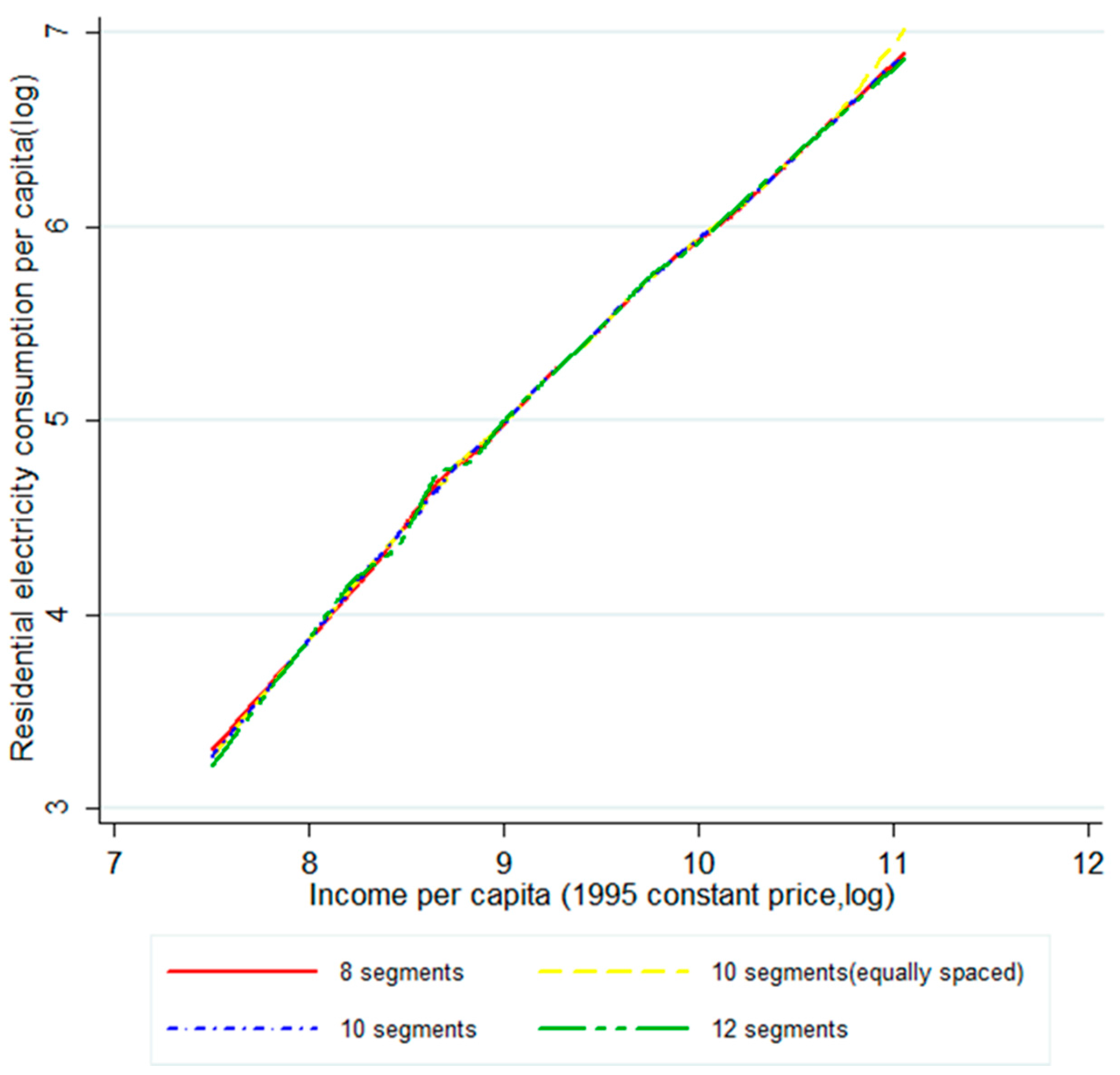
3.2.2. Segment Specifications

Segment specification primarily refers to the number of segments and segmentation methods. To test whether the results could be influenced by the number of segments in the piecewise linear model specification, we divide the income range into 8 and 15 segments by percentile in addition to 10 segments. Furthermore, we segment the income range into 10 equidistant interval ranges to determine whether the results are sensitive to the segmentation method. To better display the results of the four segment specifications, we plot the income effects in Figure 5 rather than listing the coefficients of each income segment. The four curves nearly coincide, demonstrating that the estimated results are nearly identical. Thus, we can conclude that the model specification has no effect on the results.

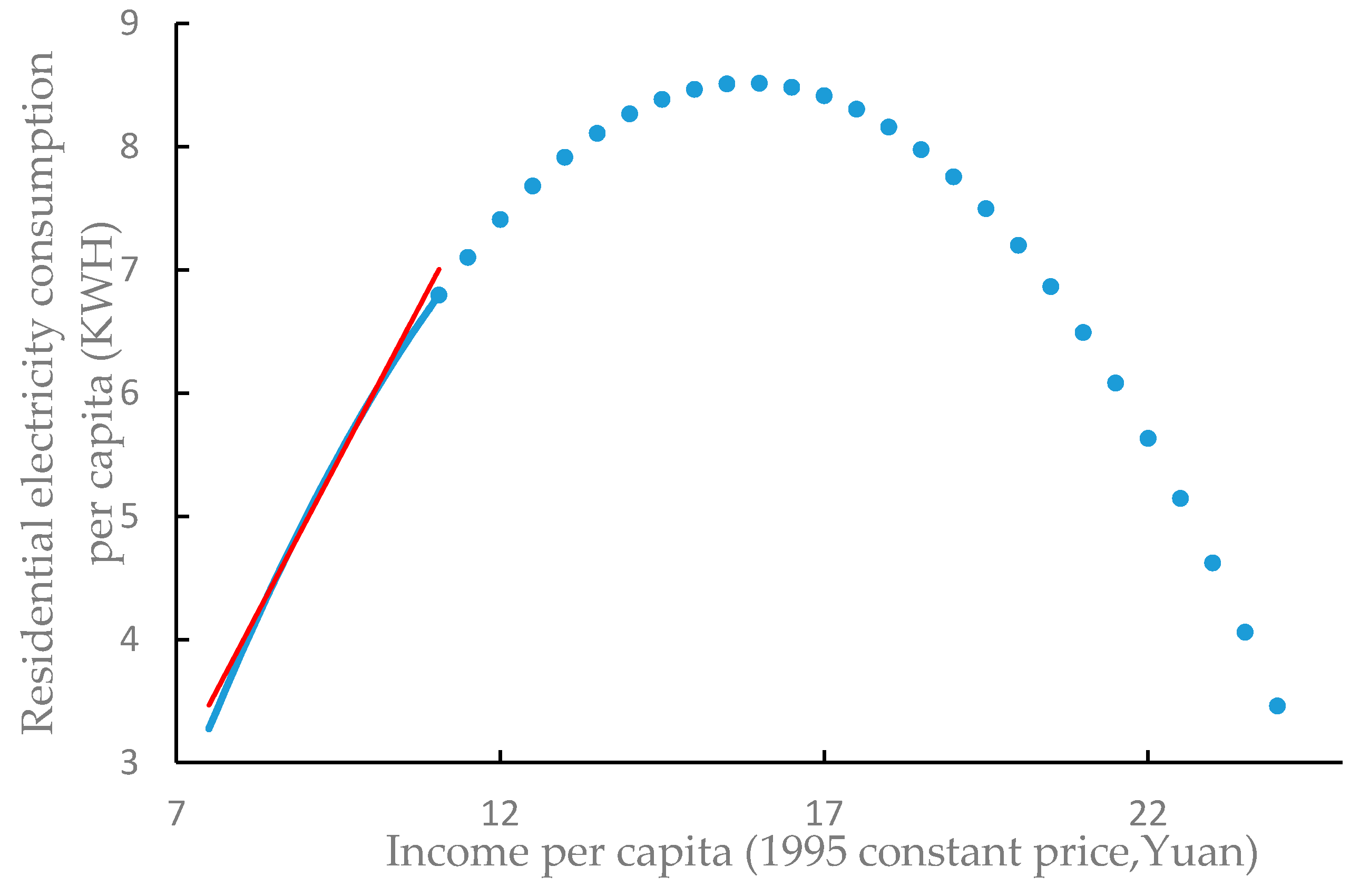
4. Comparisons and Discussion

In the empirical study above, we employ the flexible and self-adaptive piecewise model to investigate the unambiguous relationship of residential electricity consumption and income in China. To compare with the piecewise linear model, the linear and squared double-logarithmic forms that previous studies have commonly used are also estimated respectively, as presented below. All variables in Models (2) and (3) have the same interpretation as those in Model (1).
ln E i t = α 0 + α i + β ln ( Y i t ) + ε i t
ln E i t = α 0 + α i + β 1 ln ( Y i t ) + β 2 ( ln Y i t ) 2 + ε i t
Model (2) restricts the relationship between residential electricity consumption and income to be linear by a constant elasticity β . Model (3) adds a quadratic term of income, confining the relationship to nonlinearity with a turning point. In particular, if β 1 > 0 and β 2 < 0 , then we find an inverted U-shaped environmental Kuznets curve (EKC), which is widely used to capture the relationship between income and the use of natural resources or the emission of pollutants [20].
The estimation results of Models (2) and (3) are reported in Table 5. The results of Model (2) indicate that income has a significantly positive effect on residential electricity consumption with unit elasticity. In particular, we note that this finding is consistent with that obtained earlier using the piece-wise linear model, which provided strong support for our robust conclusion. In Model (3), the signs of β 1 and β 2 are positive and negative, respectively, and all coefficients are statistically significant.
The graphs in Figure 6 provide a visual representation of the estimated income effects of Models (2) and (3). Even though Model (3) displays an inverted U-shaped relationship, it is obvious that the income turning point, at which the residential electricity consumption begin to slow within the sample income range, has not been reached. Moreover, we have no knowledge whether the path of income effect will continue along the inverted U-shape out of sample. Therefore, if we had employed Model (3) in our study, a misleading conclusion could have been reached that an inverted U-shaped relationship exists between residential electricity and income in China.
Without convincing theoretical support, a fixed model form is vulnerable to producing misleading conclusions. However, the piecewise linear model that we adopted in this paper is data-adaptive and highly flexible, and it circumvents the problem of “prior restrictions” evident in Models (2) and (3). Hence, the model that we employed is reasonable, and the conclusion is robust.

5. Conclusions and Policy Implications

Using province-level panel data for the 1995–2012 period, this study investigates the relationship between residential electricity consumption and income in China. Superior to existing related studies, the current study employs a piecewise linear model that can flexibly capture the underlying relationship between the interested variables. Taking different types of segment specifications and regression methods into consideration, robust tests are carried out to ensure the validity of the research. Finally, we reach a strong conclusion that the income elasticity was approximately one and that it remained fairly stable over the estimation period. This result demonstrates that the per capita residential electricity consumption increased proportionally with the income growth of Chinese residents from 1995 to 2012. The income threshold at which residential electricity consumption automatically remains stable or slows has not been reached.
Our estimate of income elasticity exceeds most previous estimates focusing on China or other countries. The primary reason for this difference is that our model does not include control variables. The effects of such variables can be manifested in income elasticity, although they are weak. Notably, the low level of income is another reason that our model omits control variables. At low income levels, residents will allocate more money to satisfy their electricity needs as their incomes increase, leading to high income elasticity. However, when the income reaches a certain threshold that enables households to possess energy-efficient appliances sufficient to meet their needs, the level of residential electricity consumption will be stable or decline, thus reducing the income elasticity. The per capita income of Chinese residents is much lower than that of more developed countries. A large margin remains for China’s citizens to acquire more numerous and efficient appliances to satisfy their electricity demands.
Our study and its results imply that considerable changes must occur before we can observe stability or decreases in the level of residential electricity consumption in China. Therefore, to ensure the sustainable development of the electric power industry, introducing higher energy efficiency standards for electrical appliances and improving income levels are vital [10]. In addition, the government should emphasize electricity conservation in the industrial sector rather than in the residential sector. Further research is needed to determine the threshold for Chinese residential electricity consumption decreases beyond a certain income level.

Acknowledgments

We thank the financial supports from the “Strategic Priority Research Program” of the Chinese Academy of Sciences (No. XDA05150600), China’s National Key R&D Program (2016YFA0602603, 2016YFA0602801), National Natural Science Foundation of China (No. 71322306, 71273027, 71521002, 71403015, 71673026).

Author Contributions

The manuscript has been read and approved by all named authors. Hua Liao conceived and designed the research, Yanan Liu and Yixuan Gao performed the statistical analysis, Yanan Liu drafted the manuscript and Yu Hao made the major revision.

Conflicts of Interest

The authors declare no conflict of interest.

References

  1. Kemmler, A. Factors influencing household access to electricity in India. Energy Sustain. Dev. 2007, 11, 13–20. [Google Scholar] [CrossRef]
  2. Musango, J.K. Household electricity access and consumption behaviour in an urban environment: The case of Gauteng in South Africa. Energy Sustain. Dev. 2014, 23, 305–316. [Google Scholar] [CrossRef]
  3. Auffhammer, M.; Wolfram, C.D. Powering up China: Income Distributions and Residential Electricity Consumption. Am. Econ. Rev. 2014, 104, 575–80. [Google Scholar] [CrossRef]
  4. National Bureau of Statistics of the People’s Republic of China. China Statistical Yearbook (1996–2013); China Statistics Press: Beijing, China, 1996–2013.
  5. Department of Energy Statistics of National Bureau of Statistics of the People’s Republic of China. China Energy Statistical Yearbook (1996–2013); China Statistics Press: Beijing, China, 1996–2013.
  6. Auffhammer, M.; Steinhauser, R. Forecasting the path of US CO2 emissions using state-level information. Rev. Econ. Stat. 2012, 94, 172–185. [Google Scholar] [CrossRef]
  7. Liao, H.; Cao, H.S. How does carbon dioxide emission change with the economic development? Statistical experiences from 132 countries. Glob. Environ. Chang. 2013, 23, 1073–1082. [Google Scholar] [CrossRef]
  8. Schmalensee, R.; Stoker, T.M.; Judson, R.A. World carbon dioxide emissions: 1950–2050. Rev. Econ. Stat. 1998, 80, 15–27. [Google Scholar] [CrossRef]
  9. Alberini, A.; Gans, W.; Velez-Lopez, D. Residential consumption of gas and electricity in the U.S.: The role of prices and income. Energy Econ. 2011, 33, 870–881. [Google Scholar] [CrossRef]
  10. Blázquez, L.; Boogen, N.; Filippini, M. Residential electricity demand in Spain: New empirical evidence using aggregate data. Energy Econ. 2013, 36, 648–657. [Google Scholar] [CrossRef]
  11. Dergiades, T.; Tsoulfidis, L. Estimating residential demand for electricity in the United States, 1965–2006. Energy Econ. 2008, 30, 2722–2730. [Google Scholar] [CrossRef]
  12. Silk, J.I.; Joutz, F.L. Short and long-run elasticities in US residential electricity demand: A co-integration approach. Energy Econ. 1997, 19, 493–513. [Google Scholar] [CrossRef]
  13. Ziramba, E. The demand for residential electricity in South Africa. Energy Policy 2008, 36, 3460–3466. [Google Scholar] [CrossRef]
  14. Zhao, H.; Zhao, H.; Guo, S.; Li, F.; Hu, Y. The Impact of Financial Crisis on Electricity Demand: A Case Study of North China. Energies 2016, 9, 250. [Google Scholar] [CrossRef]
  15. Rasheed, M.B.; Javaid, N.; Ahmad, A.; Jamil, M.; Khan, Z.A.; Qasim, U.; Alrajeh, N. Energy Optimization in Smart Homes Using Customer Preference and Dynamic Pricing. Energies 2016, 9, 593. [Google Scholar] [CrossRef]
  16. Tang, X.; Liao, H. Energy poverty and solid fuels use in rural China: Analysis based on national population census. Energy Sustain. Dev. 2014, 23, 122–129. [Google Scholar] [CrossRef]
  17. World Energy Outlook 2014; International Energy Agency (IEA): Paris, France, 2014.
  18. Bollen, K.A.; Brand, J.E. Fixed and Random Effects in Panel Data Using Structural Equations Models; California Center for Population Research: Los Angeles, CA, USA, 2008. [Google Scholar]
  19. Jamasb, T.; Meier, H. Household Energy Expenditure and Income Groups: Evidence from Great Britain; University of Cambridge: Cambridge, UK, 2010. [Google Scholar]
  20. Richmond, A.K.; Kaufmann, R.K. Is there a turning point in the relationship between income and energy use and/or carbon emissions? Ecol. Econ. 2006, 56, 176–189. [Google Scholar] [CrossRef]
Figure 1. Ownership of appliances per 100 households in China’s rural and urban areas. Data source: China Statistical Yearbook 1996 [4] and China Statistical Yearbook 2013 [4].
Energies 09 00831 g001
Figure 2. Provincial residential electricity consumption per capital in 2012 (kWh). Note: It is a schematic map and does not implicate the definite boundaries. Data are obtained from China Energy Statistical Yearbook 2013 [5] and China Statistical Yearbook 2013 [4].
Energies 09 00831 g002
Figure 3. Residential electricity consumption per capita and GDP per capita. Note: It covers 538 observations of 30 provinces in mainland China during 1995–2012 (excluding Tibet due to lacking too many data). The per capita income was an approximate alternative to per capita GDP and adjusted to 1995 constant price.
Energies 09 00831 g003
Figure 4. Estimated income effect on residential electricity consumption. Note: The income range has been divided into 10 segments by percentile so each segment contains the same number of observations. The residential electricity consumption per capita on the vertical axis has been adjusted for the effect of income excluding the province-fixed effect.
Energies 09 00831 g004
Figure 5. Estimated income effects using different segmentation. Note: 8-, 10-, 12-segment models are divided by percentile, and the 10-segment (equally spaced) model divides the income range into 10 intervals of equal width. The residential electricity consumption per capita on the vertical axis has been adjusted for the effect of income excluding the province-fixed effect.
Energies 09 00831 g005
Figure 6. Estimated income effects of Models (2) and (3). Note: The residential electricity consumption per capita on the vertical axis has been adjusted for the effect of income, excluding the province-fixed effect. The red solid line captures the estimated income effects of Model (2) in the sample. The blue solid line and dotted line capture the estimated income effects of Model (3) in the sample and out of the sample, respectively.
Energies 09 00831 g006
Table 1. Electricity access in 2012: regional aggregates. Data source: IEA, World Energy Outlook 2014 [17].
RegionElectrification Rate (%)Urban Electrification Rate (%)Rural Electrification Rate (%)
Developing countries76.391.164.0
Africa42.568.025.6
Developing Asia83.095.274.4
China99.8100.099.6
India75.493.966.9
Latin America95.098.581.9
Middle East91.798.378.0
Transition economies & OECD99.9100.099.7
World81.794.168.0
Table 2. Descriptive statistics.
VariableDefinitionObservationsMeanStd. Dev.MinMax
ln(E)Residential electricity consumption per capita (kWh)5385.40.73.46.9
ln(Y)GDP per capita (Yuan)5389.50.67.511.1
Table 3. Test results for heteroskedasticity and autocorrelation.
Modified Wald Test
H0: sigma(i)^2 = sigma^2 for all iChi 2 (30) = 7442.88
Prob > chi2 = 0.0000
Wooldridge Test
H0: no first-order autocorrelationF(1, 29) = 15.722
Prob > F = 0.0004
Table 4. Estimate results of different estimate methods.
IncomeOLSIVFGLS
0–39911.211 ***1.208 ***0.905 ***
(8.43)(5.17)(9.50)
3991–51301.120 ***1.337 **1.061 ***
(4.98)(2.73)(9.72)
5130–64381.231 ***1.2151.029 ***
(4.81)(1.71)(9.58)
6438–80020.850 **0.4991.040 ***
(3.12)(0.60)(10.02)
8002–99021.101 ***1.631 *0.990 ***
(3.98)(2.02)(9.77)
9902–12,3650.888 ***0.4581.019 ***
(3.33)(0.66)(10.39)
12,365–15,2101.073 ***1.435 *1.052 ***
(3.70)(2.27)(10.35)
15,210–19,3310.895 ***0.6731.130 ***
(3.59)(1.64)(11.92)
19,331–28,5410.783 ***0.877 ***0.707 ***
(5.16)(4.68)(8.08)
>28,5410.943 ***0.894 ***0.941 ***
(7.49)(6.75)(12.43)
constant−5.818 ***−5.824 **−3.246 ***
(−4.98)(−3.07)(−4.17)
N538509538
Note: ***, ** and * indicate statistical significance at 1%, 5%, and 10%. Standard errors are in parentheses. Income ranges are divided into 10 segments by percentile so that each segment contains the same number of observations. The first lag of per capita income is chosen as the instrumental variable in the IV estimate. Province-fixed effects are not reported.
Table 5. Estimate results of Models (2) and (3).
VariablesModel (2)Model (3)
ln ( Y i t )0.996 ***2.396 ***
(58.08)(7.83)
( ln Y i t ) 2 -−0.0757 ***
-(−4.58)
constant−4.006 ***−10.44 ***
(−25.27)(−7.39)
N538538
Fixed EffectsYESYES
Random EffectsNONO
R 2 0.86940.8746
Note: *** indicate statistical significance at 1%. Province-fixed effects are not reported.

