Effects of Freestream Turbulence in a Model Wind Turbine Wake

Abstract

The flow structure in the wake of a model wind turbine is explored under negligible and high turbulence in the freestream region of a wind tunnel at $Re\sim 7\times {10}^4$. Attention is placed on the evolution of the integral scale and the contribution of the large-scale motions from the background flow. Hotwire anemometry was used to obtain the streamwise velocity at various streamwise and spanwise locations. The pre-multiplied spectral difference of the velocity fluctuations between the two cases shows a significant energy contribution from the background turbulence on scales larger than the rotor diameter. The integral scale along the rotor axis is found to grow linearly with distance, independent of the incoming turbulence levels. This scale appears to reach that of the incoming flow in the high turbulence case at $x/d\sim$ 35–40. The energy contribution from the turbine to the large-scale flow structures in the low turbulence case increases monotonically with distance. Its growth rate is reduced past $x/d\sim$ 6–7. There, motions larger than the rotor contribute ∼$50\%$ of the total energy, suggesting that the population of large-scale motions is more intense in the intermediate field. In contrast, the wake in the high incoming turbulence is quickly populated with large-scale motions and plateau at $x/d\sim 3$.

1. Introduction

Understanding the evolution of energetic coherent motions in the wake of wind turbines under various background turbulence is critical for the proper description of the unsteady interaction between turbines and the atmospheric boundary layer [1], and inter-turbines in the context of wind farms. Unsteady loading and power output fluctuations are direct consequences of the flow turbulence, which can modulate the bulk energy converted by wind farms [2].

Turbulence in the wake of wind or hydrokinetic turbines is known to be determined by the characteristics of the incoming flow and the rotor-generated motions. Special attention has been placed in characterizing the mean velocity [3,4] and turbulence intensity $I_u$ [5,6] in the wake of wind turbine(s). Various studies have focused on characterizing $I_u$ along the rotor axis [7,8,9]. In general, $I_u$ is expressed in terms of the incoming turbulence $I_0$, and the added turbulence in the wake $I_{+}$, such that $I_u^2=I_0^2+I_{+}^2$. A recent work by Ozbay et al. [10] reported that high $I_u$ can enhance the total power output of a wind farm. Field experiments using nacelle-mounted Lidar systems [11] and Sodar [12] have provided insight on the velocity fluctuations at full scale, accounting for meandering motions.

While the mean velocity deficit and bulk turbulence levels provide key information about wind turbine wakes, detailed insight into the structure of the velocity fluctuations is necessary in order to better understand the underlying dynamics of such flows. In particular, the quantification of the scale-by-scale interaction of the wake and outer flow is required to estimate turbine behavior within wind farms. For example, based on experimental results and numerical simulations, Crespo and Herna [8] proposed a spectrum model for the evolution of wind-turbine wakes. Medici and Alfredsson [13] reported the existence of the meandering effect, presented as a low-frequency component in spectra (see also [14]). Chamorro et al. [15] described the turbine as an “active filter” of the flow due to their effect in modulating the large- and small-scale turbulence. Furthermore, Singh et al. [16] argued that the wind turbines reduce the asymmetry and intermittency in the wake flow, resulting in more homogenized velocity fluctuations as compared to the base flow. From a series of recently conducted experiments, Chamorro et al. [17] analyzed the evolution of the large-scale turbulence in the wake of a hydrokinetic turbine, and proposed a new approach to quantifying the wake recovery based on the development of the integral scales, showing that strong coherent motions are more effective than turbulence levels for triggering the break-up of the spiral structure of the tip-vortices [18]. This reveals the influence of energetic motions in the wake characteristics and the power output, which are essential to better assess environmental aspects and establish robust engineering models.

As discussed above, a direct effect of the wake unsteadiness is the power output fluctuation in single turbines and wind farms. Measurements by Apt [19] showed that the spectrum of wind farm power fluctuations follows a power-law behavior consistent with the inertial subrange of the turbulence. A similar phenomenon was observed by Milan et al. [20] in the low frequency range. Chamorro et al. [21] showed that the spectral content of the power distribution of a MW size wind turbine contains three distinctive regions. In the first region—defined by subrotor length scales—the turbine power is insensitive to the turbulence. In the intermediate region—with length scales up to those on the order of the atmospheric boundary layer thickness—the spectral contents of the power fluctuations ${\mathrm{\Phi }}_P$ and flow ${\mathrm{\Phi }}_U$ exhibit a non-linear relationship that can be characterized by a transfer function $G\left(f\right)\propto f^{-2}$. In the third region—dominated by very large scales—the power fluctuations are found to be directly influenced by the flow. Recently, Tobin et al. [22] established a tuning-free model for the transfer function $G\left(f\right)$, which shows robust performance across wind turbine sizes spanning from laboratory models to MW scales.

The main goal of this paper is to provide more insight on the wake characteristics of a model turbine under two significantly different turbulence intensities. The experimental setup is described in Section 2; analysis, results, and discussion are presented in Section 3; and conclusions are provided in Section 4.

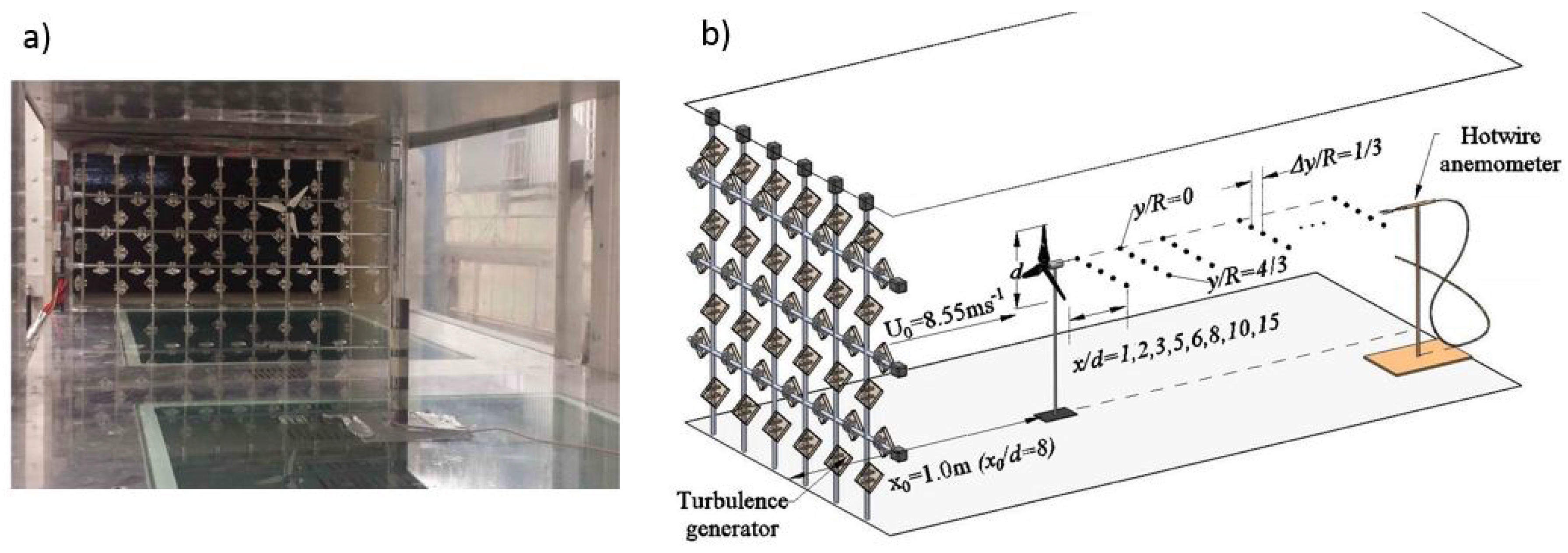
2. Experimental Setup

The experiment was conducted in the wind tunnel of the University of Illinois at Urbana-Champaign’s Renewable Energy and Turbulent Environment Group. The Eiffel-type wind tunnel test section is 0.914 m wide, ∼0.46 m high, and 6.10 m long. The ceiling is fully adjustable to control the pressure gradient along the test section, which is set to nearly zero during the experiment. More details of the facility can be found in Adrian et al. [23]. A miniature turbine was placed near the beginning of the test section ($x_0$ = 1 m from the inlet) at the center of the test section, within the freestream region of the flow, and operated under two distinctive turbulence levels.

The rotor diameter of the horizontal-axis model wind turbine was $d=$ 0.12 m, having $P_0\approx$ 1 W rated power, and was based on the reference model from Sandia National Labs [24]. The blades and nacelle were made of PolyJet Vero material and fabricated at the University of Illinois Rapid-Prototyping Lab using an Objet Eden 350 machine. The basic geometry of the blades is given in

Table 1. Basic geometry of the model wind turbine blades; c denotes the chord length, α represents the angle with respect to the rotor plane, and r and R are the radial distance and rotor radius.

$\mathit{r}/\mathit{R}$	$0.2$	$0.3$	$0.4$	$0.5$	$0.6$	$0.7$	$0.8$	$0.9$	$0.95$
$c/R$	$0.275$	$0.248$	$0.215$	$0.181$	$0.156$	$0.136$	$0.119$	$0.100$	$0.088$
$\alpha (°)$	$31.8$	$23.9$	$17.7$	$12.8$	$9.4$	$7.5$	$6.0$	$4.6$	$3.9$

. A Precision Microdrives 112-001 Micro Core 12 mm DC Motor was used as a loading system (generator). The angular velocity of the rotor Ω was controlled by the resistance of the generator, which was set to 2 ohms. The mean incoming velocity for all cases was $U_0=8.5$ m·s${}^{-1}$, giving a Reynolds number based on the rotor diameter of $Re=Ud/\nu \sim 7\times {10}^4$, where ν is the kinematic viscosity, and a tip-speed ratio $\lambda =\mathrm{\Omega }R/U_0$ = 5. More details on the model turbine and its performance can be found in Tobin et al. [22].

An active turbulence generator ($TG$) was used to induce large-scale and energetic coherent motions, resulting in high-turbulence (henceforth $HT$) intensity $I_{HT}={\sigma }_u/U_0\approx 11.5\%$ at the turbine location. Here, ${\sigma }_u$ is the standard deviation of the streamwise velocity fluctuations. In contrast, very low turbulence (henceforth $LT$) intensity $I_{LT}\approx 0.2\%$ without the $TG$ is obtained at the turbine location. The $TG$ uses 13 stepper motors, independently controlled by an Arduino microcontroller. Each stepper motor rotates one of the three horizontal rods and ten vertical rods fitted with agitator wings, which were turned at 1 rev·s${}^{-1}$ and randomly changed direction at a frequency of 0.2 Hz. The horizontal and vertical rods are spaced $M=90$ mm apart, where nine and four square blocks are attached to each horizontal and vertical rod. The rigid square blocks are 28 mm long and 5.5 mm thick. A basic schematic of this $TG$ is illustrated in Figure 1a. Constant temperature hot-wire anemometry (CTA) was used to obtain high-resolution measurements of streamwise velocity at various positions downwind of the turbine. The hotwire was made of 5.0 $\mathsf{\mu }$m tungsten wire, and connected to a Dantec dynamics system. The signals were sampled at frequency $f=20$ kHz for a measurement period of 120 s, and low-pass filtered at 2.5 kHz. Calibration of the probe was conducted against a pitot tube. Through the calibration and experiment, the temperature was kept at 24 ${}^{\circ }$C within ±0.5 ${}^{\circ }$C to avoid thermal drift of the voltage signal. The measurement locations included near and far wake regions containing spanwise profiles $y/R=0,1/3,2/3,1,4/3$ at streamwise locations $x/d=1,2,3,5,6,8,10,15$, where the origin of the coordinate system $(x,y)=(0,0)$ was located at the center of the rotor.

3. Results and Discussion

In this section, we characterize the sensitivity of the turbine wake to the incoming turbulence levels. Changes in the mean statistics, spectral content, and integral length scales of the flow are used for this purpose. Before exploring the structure of the wake, it is worth stressing the sensitivity of the mean velocity deficit, $\Delta U=U-U_0$, with turbulence levels. As is known, background turbulence promotes mixing, momentum exchange between the wake and outer flow, which results in faster wake recovery. This phenomenon is particularly relevant to the wake behavior during the diurnal cycle, where stable thermal stratification at night time results in lower turbulence and longer turbine wakes [25].

Figure 2 illustrates selected spanwise profiles from the rotor axis of the mean velocity deficit $\Delta U/U_0$ within the near wake region. In general, the difference of velocity deficit between the $HT$ and $LT$ increases with the distance from the rotor up to about $x/d\sim$5, and gradually decreases in the far wake. This is strongly linked with the entrainment and interaction of the large-scale motions with the wake.

The turbulence interaction between wake and outer flow is expected to be closely linked not only with the turbulence levels of the outer flow, but also with the structure of the turbulence. This is inspected via the velocity spectra, and real-space autocorrelations at various locations downwind of the model turbine.

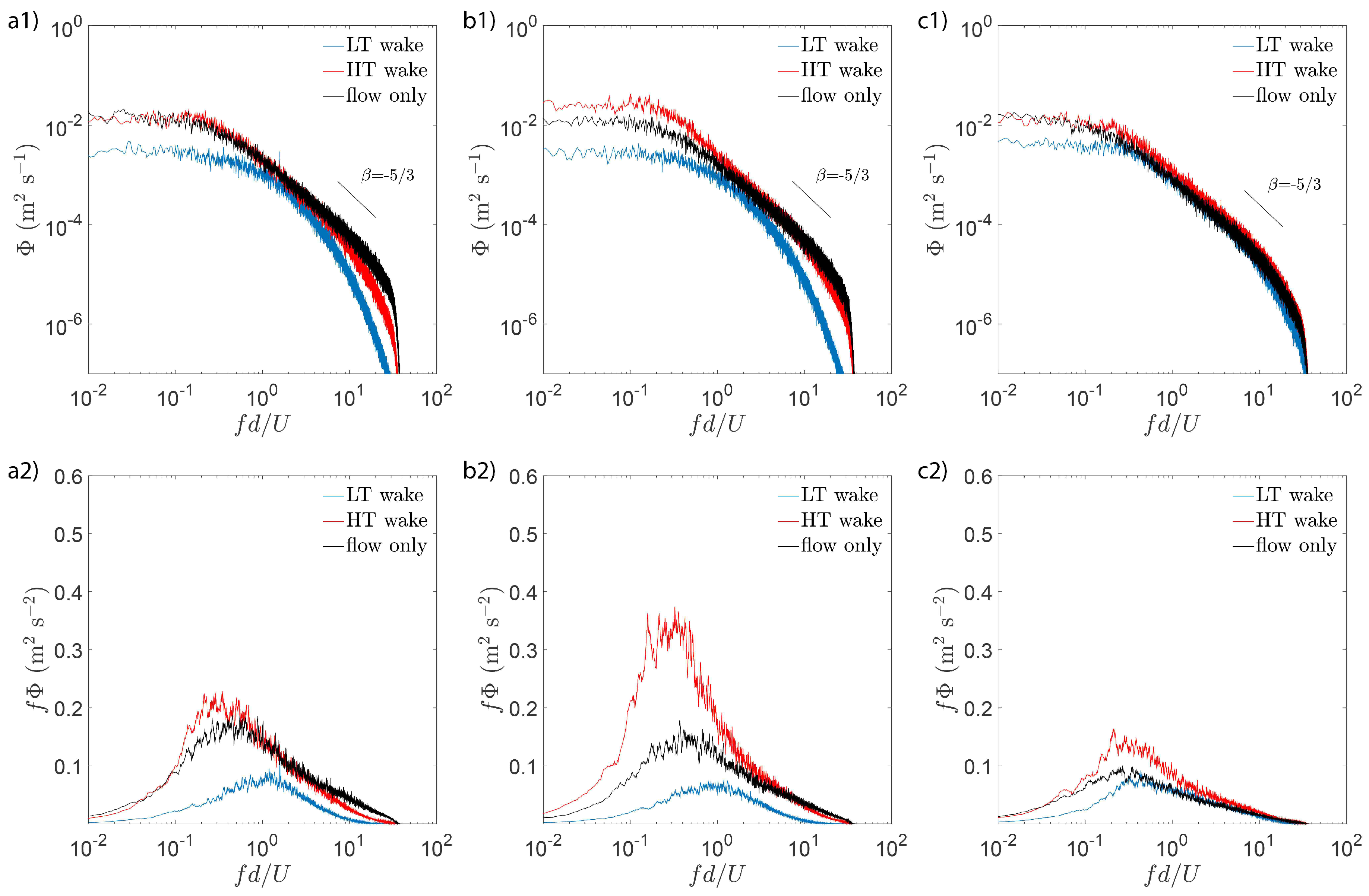
3.1. Background Turbulence Modulation on the Wake Velocity Spectra

In order to quantify the role of background turbulence on the structure of the velocity fluctuations in the turbine wake, we first characterize the velocity spectra (${\mathrm{\Phi }}_u$) at several locations along the rotor axis ($y/R=0$). Figure 3 illustrates ${\mathrm{\Phi }}_u$ in the near and far wake regions at $x/d=$ 2, 3, and 10. To aid comparison, the $HT$ and $LT$ cases are superimposed, while the spectrum of the high-turbulence flow without the turbine is included as a reference. The incoming flow in the $HT$ case exhibits a distinctive inertial subrange ($\mathrm{\Phi }\propto f^{-5/3}$) that roughly extends two decades, and energetic motions larger than the turbine rotor, as illustrated in the $f\mathrm{\Phi }$ set in Figure 3. This feature allows important geometrical similarities with full-scale setups to be mimicked, as will be discussed later. In general, the turbine wake exhibits a similar energy cascade, except very near the rotor in the $LT$ case (Figure 3a1). In this case, the dynamics is mostly modulated by the rotor, and the turbulent interaction with the outer flow is minimum. It is important to note that in the far field, the wake in the $LT$ case has developed both large- and small-scale motions (Figure 3c1). The large-scale motions are associated (among other phenomena) to wake meandering [17,26], while the development of small-scale structures (e.g., sub-rotor, $fd/U\ge 5$) is due to the production of the turbulence kinetic energy induced in the shear layer of the wake. Similar phenomena have been reported for other setups, including flow passing circular and rectangular cylinders, spheres, among others [27,28,29].

The differences between the cases across scales are highlighted with the corresponding pre-multiplied spectra $f\mathrm{\Phi }$ in Figure 3(a2–c2). The structure of the turbulence generated by the turbine under very low turbulence background ($LT$ case) in the very near wake at $x/d=2$ exhibits the lowest energy across the reduced frequencies analyzed, and shows a peak at a length scale on the order of the turbine diameter. Interestingly, the $HT$ case exhibits more energy in the large-scale motions contained within $fd/U\in [{10}^{-1},{10}^0]$ than the turbulence without the turbine. This suggests a strong interaction between the flow and turbine wake, where the sharp shear layer is subject to strong instability. The difference increases with distance within the near wake and decreases in the far field, but is still significant at $x/d=10$. The $HT$ and flow-only cases show a spectral peak around $fd/U\sim 0.3$, which indicates a length scale of roughly three rotor diameters. This scale is further inspected later with the correlation function.

Overall, the differences between the spectral distributions of the velocity fluctuations in the $HT$ and $LT$ cases are not fully attributed to the higher incoming flow turbulence intensity; the structure of such fluctuations is also an important factor. It is worth noticing that in Chamorro et al. [15], a turbine placed in a non-uniform flow (boundary layer) is defined as an active filter able to amplify the small-scale motions while damping the large-scale ones. Comparison of the spectral energy distribution from experiments by Chamorro et al. [15] with this work indicates that the energy amplification within the range $fd/U\in [{10}^{-1},{10}^0]$ exists in both cases, but near the tip in the case of Chamorro et al. [15] (boundary layer flow). This shows the strong role of the wall in modulating the structure of the flow. Further inspection at various spanwise locations shows that the amplification effect is maximized at around $y/R=2/3$ (Figure 4). Note that the peaks near the blades tip at $y/R$=2/3 and 1 in Figure 4b,c correspond to the rotor frequency $f_T$ and its harmonics.

The bulk differences between the spectra of the $HT$ and $LT$ cases can be directly inferred from the differences between the corresponding variances ${\sigma }_{HT}^2$ and ${\sigma }_{LT}^2$. This quantity ($\Delta {\sigma }^2={\sigma }_{HT}^2-{\sigma }_{LT}^2$) is equivalent to the so-called added turbulence $I_{+}^2$ discussed in Section 2. Figure 5 illustrates $\Delta {\sigma }^2$ normalized with that of the local flow without turbine, ${\sigma }_f^2$, for various streamwise and spanwise locations. It reveals a similar trend over all spanwise directions, and shows that the difference increases with distance within the near wake, and reaches a maximum at $x/d\sim 3$. Past this location, $\Delta {\sigma }^2$ decreases in a non-linear way. To further highlight these differences across scales, the pre-multiplied spectral difference, $\Delta \left(f{\mathrm{\Phi }}_u\right)=f{\mathrm{\Phi }}_{HT}-f{\mathrm{\Phi }}_{LT}$, is shown in Figure 6 for various streamwise and spanwise locations. A significant energy increase induced by the high background turbulence is clearly observed in the normalized frequency range $fd/U\sim [{10}^{-1},{10}^0]$. This energy growth is most distinct around the turbine tip ($y/R\sim 2/3-1$), as suggested in Figure 5, and highlights the role of the background turbulence on influencing the energy content of the large-scale motions within distances common in wind farm setups.

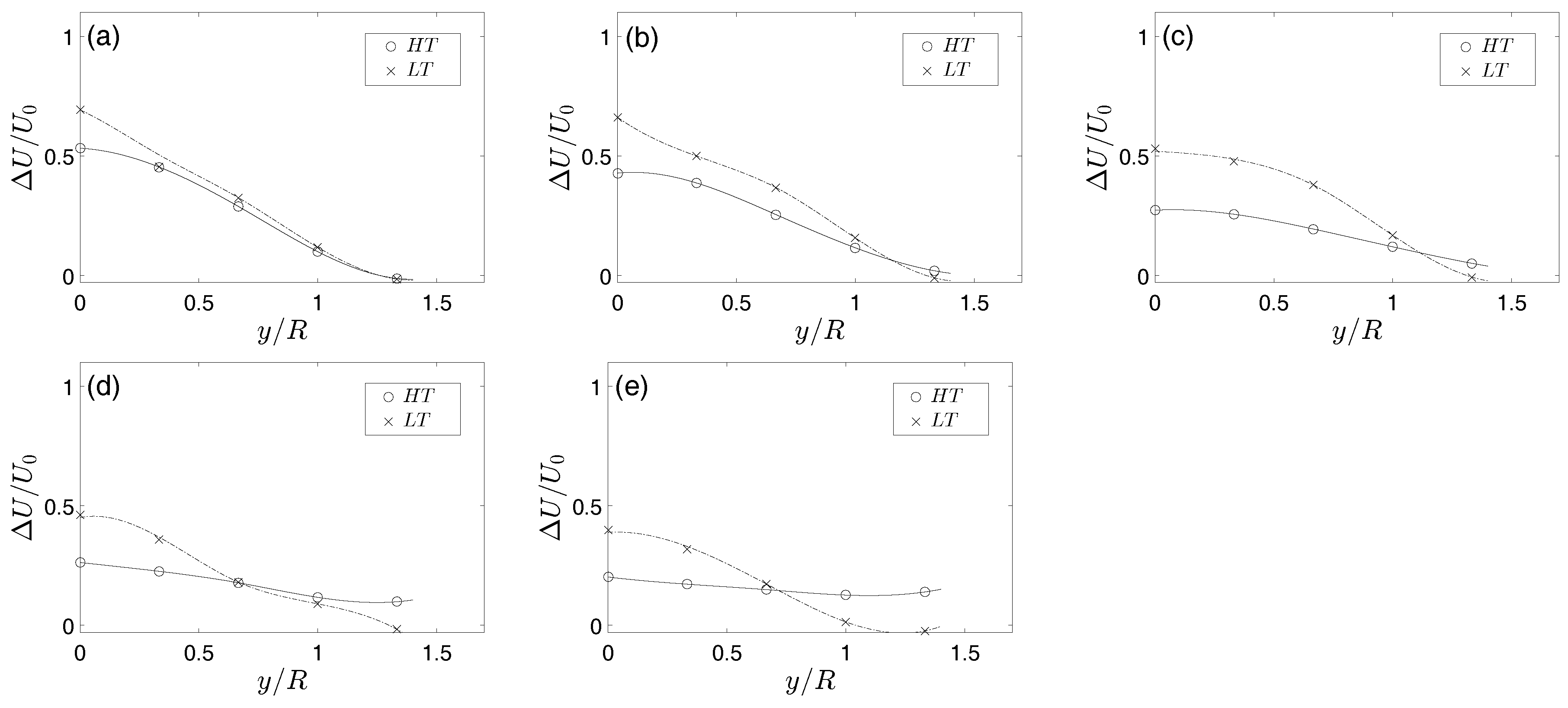
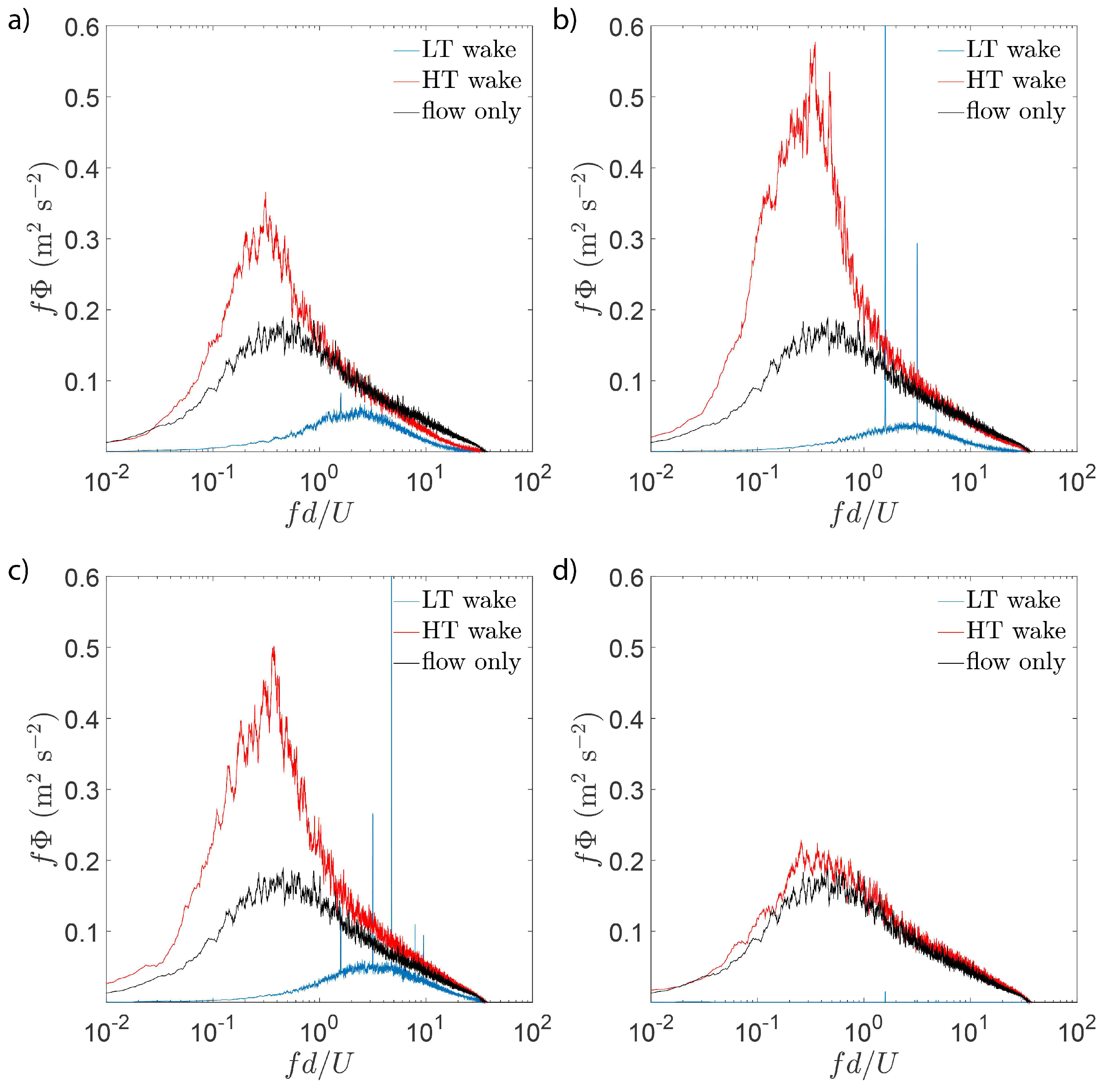
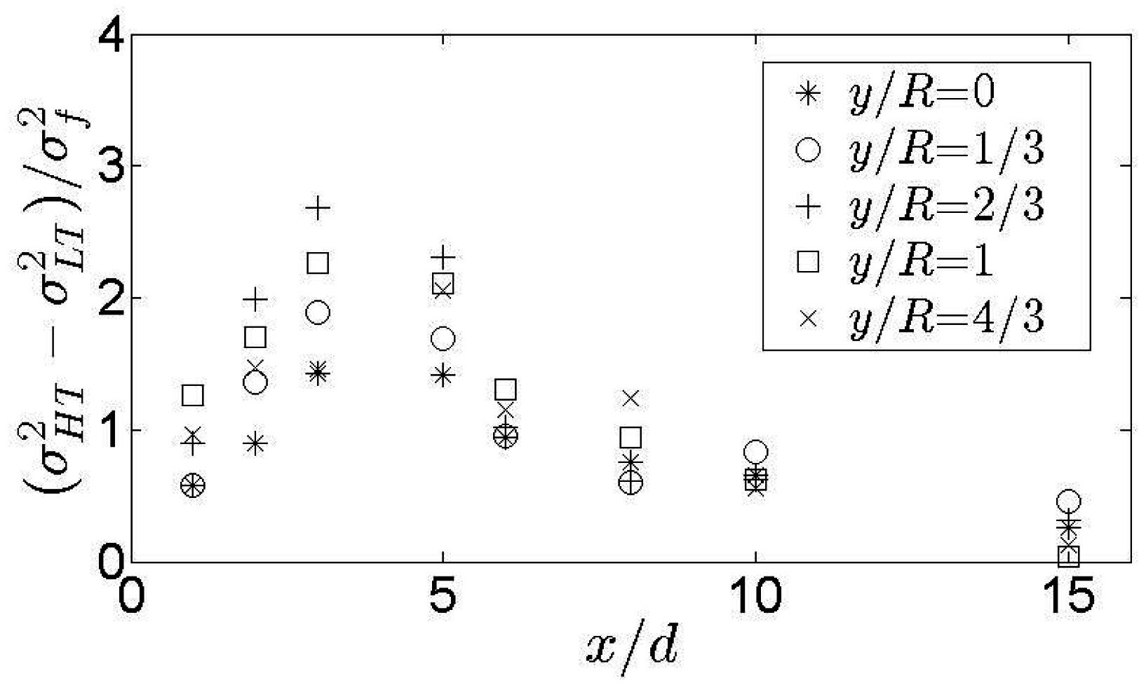
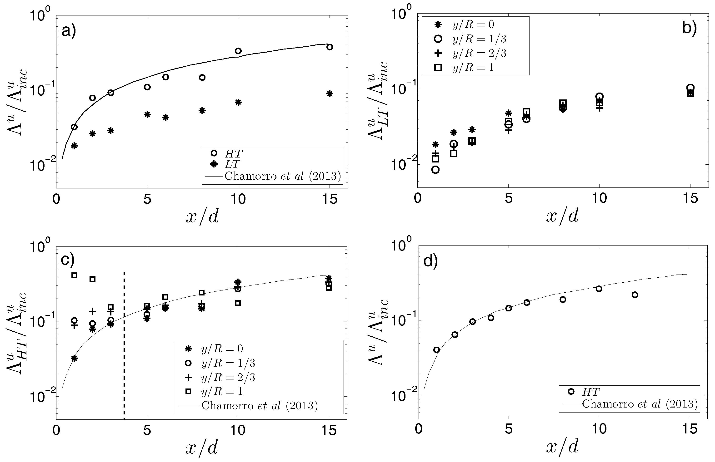
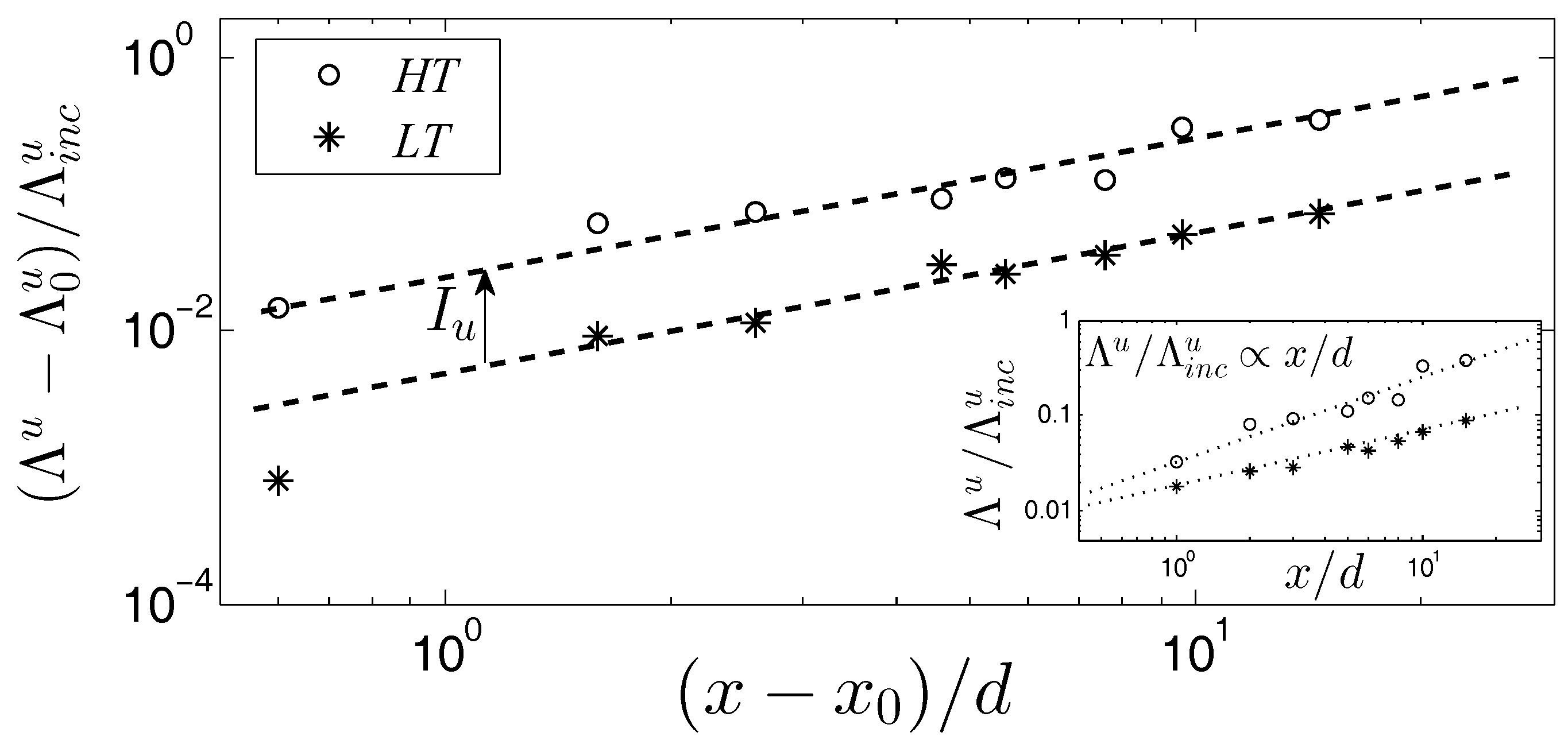
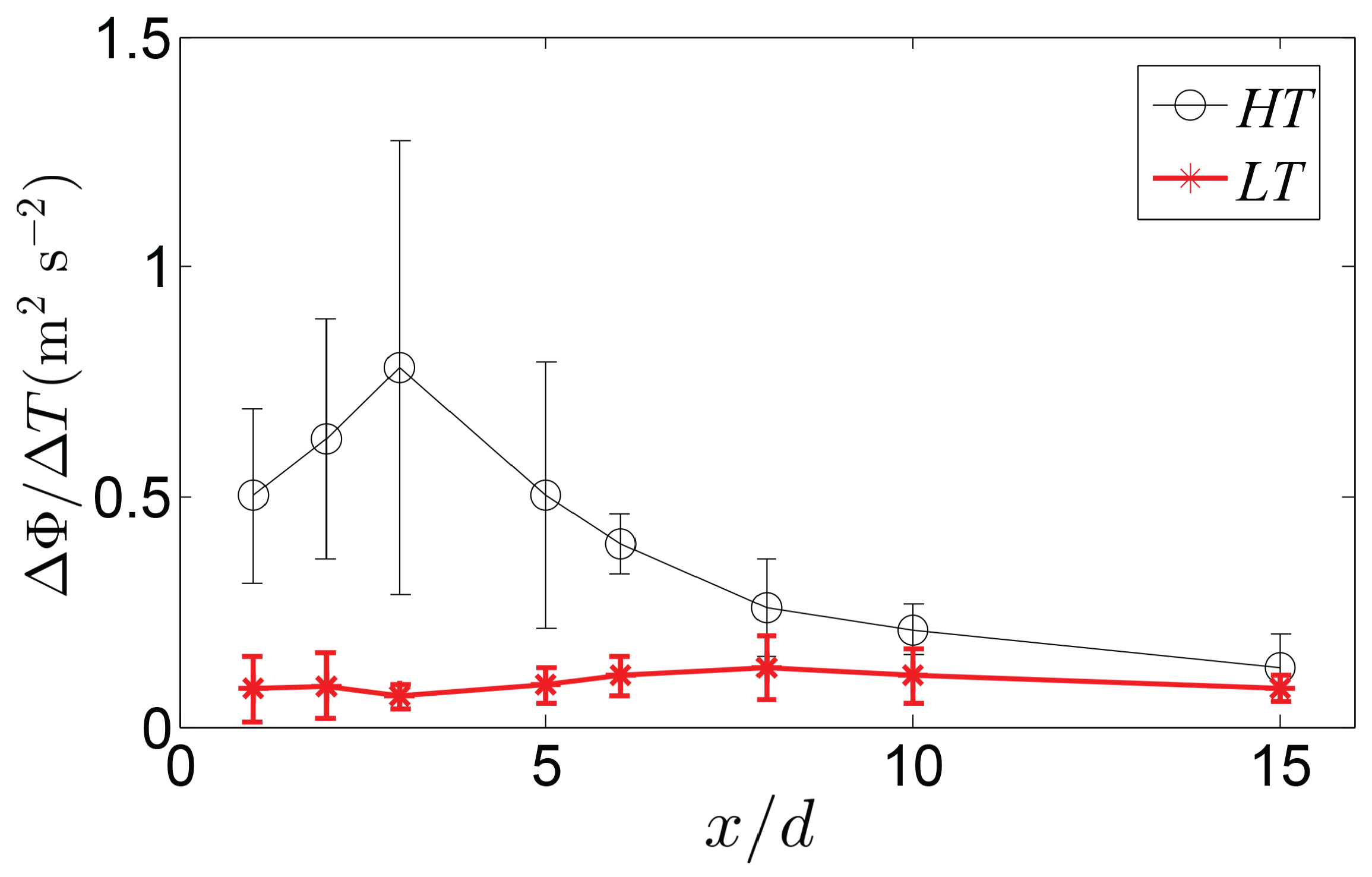
3.2. Evolution of the Large-Scale Motions

The evolution of the integral length scale ${\mathrm{\Lambda }}^u$ is described in terms of the autocorrelation function of the streamwise velocity fluctuations, $r\left(\tau \right)$, as follows:

$$\begin{array}{c}\hfill r\left(\tau \right)=\overline{u^{\prime }\left(t\right)u^{\prime }(t-\tau )}/{\sigma }_u^2,\\ \hfill T^u=\underset{0}{\overset{\infty }{\int }}r\left(\tau \right)d\tau ,\\ \hfill {\mathrm{\Lambda }}^u=U{T}^u,\end{array}$$

(1)

where τ is the time lag and U is the local velocity. Note that the autocorrelation function $r\left(\tau \right)$ can be related to power spectra $\mathrm{\Phi }\left(\omega \right)$ via $\mathrm{\Phi }\left(\omega \right)={\int }_{-\infty }^{+\infty }r\left(\tau \right)e^{-i\omega \tau }d\tau$. The incoming flow field in the $HT$ setup (i.e., with the turbulence generator) is ${\mathrm{\Lambda }}_{inc}^u/d=2.5$. This scale is on the order of that observed in the field for MW turbines, where $d\sim$ 100 m and ${\mathrm{\Lambda }}^u\sim$ 300 m [30]. It is worth pointing out the role of active grids on the generation of large turbulent scales and extended inertial subrange in freestream turbulence [26,31]. These elements are necessary to uncover the rich multi-scale dynamics in turbine wakes with the surrounding flow.

The evolution of ${\mathrm{\Lambda }}^u$ in the turbine wake was obtained at various streamwise and spanwise locations, and normalized by that of the incoming flow ${\mathrm{\Lambda }}_{inc}^u$. This is shown in Figure 7a for both the $LT$ and $HT$ cases along the axis of the rotor ($y/R=0$). The experiments from Chamorro et al. [17] in a turbulent, low-shear open channel flow is also included as a reference. Remarkably, ${\mathrm{\Lambda }}^u$ coincides well with those experiments, which also have similar incoming turbulence ($I_u\sim 12\%$) and ${\mathrm{\Lambda }}_{inc}^u/d$ (=3.4). This suggests that these two quantities play a dominant role on the evolution of the integral length scale. The difference of ${\mathrm{\Lambda }}^u$ between the $HT$ and $LT$ cases increases with the downwind distance and, as shown later in Figure 8, this increase is linear such that:

$$\begin{array}{c}{\frac{\partial {\mathrm{\Lambda }}^u}{\partial x}}_{{|}_{LT}}\approx 0.005\frac{{\mathrm{\Lambda }}_{inc}^u}{d},\mathrm{and}\\ {\frac{\partial {\mathrm{\Lambda }}^u}{\partial x}}_{{|}_{HT}}=5{\frac{\partial {\mathrm{\Lambda }}^u}{\partial x}}_{{|}_{LT}}.\end{array}$$

(2)

The distribution of ${\mathrm{\Lambda }}^u$ in other spanwise locations is displayed in Figure 7b,c for the $LT$ and $HT$ cases. In the $LT$ case, ${\mathrm{\Lambda }}^u$ is not very sensitive to the spanwise coordinate $y/R$, which is due to the fact that the turbulence is induced along the rotor without external modulation. Between $x/d=1$ to 15, ${\mathrm{\Lambda }}_{LT}^u$ increases from ∼10${}^{-2}{\mathrm{\Lambda }}_{inc}^u$ to ∼10${}^{-1}{\mathrm{\Lambda }}_{inc}^u$ (i.e., from ∼blade chord length to $R/2$). Conversely, comparatively large variability of ${\mathrm{\Lambda }}^u$ in the $HT$ case occurs in the spanwise direction within the near wake up to about $x/d\sim$ 3–4, as illustrated in Figure 7c. Close to the turbine and near the tip, the integral scale is significantly influenced by the large scales of the background flow. Figure 7c also shows the reduction of spanwise variability past $x/d\sim 4$, which is the effect of the mixing coupled with increasingly larger turbulence scales generated by the turbine (from Figure 7b). To account for potential effects in the interaction between wake and the background flow due to turbulence decay with downwind distance, additional experiments were performed by moving the turbine upwind while fixing the hotwire. This is shown in Figure 7d, where results from Chamorro et al. [17] are also included as a reference. The trend is very similar to the other case, which indicates that the evolution of the integral scales is not affected by the setup.

Figure 8 (and inset) shows the approximately linear relation of ${\mathrm{\Lambda }}^u$ with distance in the region of interest. Note that extrapolation of the trend over the $HT$ case suggests that ${\mathrm{\Lambda }}^u$ reaches that of the incoming flow ${\mathrm{\Lambda }}_{inc}^u$ at about $x/d\sim$ 35–40, and the differences between the $LT$ and $HT$ cases become the same at $x_0/d\sim 1/8$ (i.e., ${\mathrm{\Lambda }}_{LT}^u={\mathrm{\Lambda }}_{HT}^u={\mathrm{\Lambda }}_0^u$). Within this very near wake region, the signature of the outer flow is completely absent. Then, the relative quantities $({\mathrm{\Lambda }}^u-{\mathrm{\Lambda }}_0^u)$ and $(x-x_0)/d$ appears as parallel lines in log–log scale for the $HT$ and $LT$ cases, where the offset is a direct effect of the characteristic slope $\partial {\mathrm{\Lambda }}^u/\partial x$ (Equation (2)). The consistent linear growth of the integral length scale despite the level of the background turbulence has important applications in full-scale systems. It allows for its characterization with limited data and the use of turbulence spectrum models (such as von Kármán [32]) in the wake of wind turbines or within wind farms. Figure 9 shows the energy contribution from overall large-scale flow structures ${\sigma }_{lp}^2$ for the $LT$ and $HT$ cases; here, subindex “$lp$” denotes low-pass filtering. The cut-off frequency was that corresponding to the rotor size (i.e., $f_{lp}=U_c/d$), where $U_c$ is the local mean velocity. As can be seen from this figure, the energy contribution from the turbine to the large scale flow structures in the $LT$ case increases monotonically with distance. As indicated by the dashed trend lines, the growth rate $\partial {\sigma }_{lp}^2/\partial x$ in the $LT$ is reduced past $x/d\sim$ 6–7. At this location, the large scale motions contribute roughly 50% of the total energy. This suggests that the population of large-scale motions is more intense within the intermediate field rather than in the far field. In contrast to the $LT$, the wake in the $HT$ is quickly populated with large-scale motions and plateaus at $x/d\sim$ 3. In addition, energy contribution is overall higher (as documented earlier) in the case of $HT$ as compared to the $LT$ case.

To further explore the interaction of turbine with large-scale flow structures and their persistence, we reconstruct low-pass filtered time series for the scales between maximum energy observed in velocity spectra (Figure 3) and the integral length scales. We then compute the energy decay rate ($\Delta \mathrm{\Phi }/\Delta T$) of these large-scale flow structures as a function of downwind distance for both $HT$ and $LT$ wakes (Figure 10). Similar to Figure 9, a peak is observed in Figure 10 in the $HT$ case, showing maximum energy decay rate at $x/d\sim$ 3. However, this figure reveals a contrasting decrease in energy decay rate for both mean and standard deviation (depicted by the error bar lines) for the $LT$ wake (at $x/d\sim$ 3), suggesting that the large-scale flow structures possess lower temporal correlation in the case of $LT$ wake than in the $HT$ wake. In other words, at $x/d\sim$ 3, the interaction between large-scale flow structures increases in $HT$ wakes, whereas it decreases in $LT$ wakes. At a downwind distance of $x/d\sim 8$, the decay in the $HT$ case tends to converge towards the decay rate in the $LT$ case.

4. Conclusions

The structure of a model wind turbine wake was inspected under two conditions sharing the same mean flow, but exhibiting very distinctive turbulence levels. In one of the cases, the incoming flow had negligible turbulence ($I_u\sim 0.2\%$); whereas in the other case, $I_u\sim 11.5\%$. The comparison of these two cases allowed us to obtain insight into the effect of background turbulence on the evolution of the integral length scale and contribution of the large-scale motions in the velocity fluctuations.

As expected, results show that background turbulence plays a central role in the flow recovery in the turbine wake. The compensated spectra of the velocity fluctuations in the low-turbulence case exhibits the lowest energy across scales the in the very near wake, with peak at a scale corresponding to the rotor diameter. In contrast, the high turbulence case shows more energy in the range $fd/U\in [{10}^{-1},{10}^0]$, which is larger than the incoming turbulence. Regardless of the turbulence levels, the integral scale along the axis of the rotor is found to grow linearly with distance from the turbine. In addition, the growth rate of the integral scale in the high turbulence case was five times larger than that with the negligible background turbulence. Future characterization of this scale under other turbulence levels and assessment of wall effect will allow the development of simple parametrization for the description of the structure of wind turbine wakes.

References

1. Chamorro, L.P.; Sotiropoulos, F. Turbulent flow inside and above a wind farm: A wind-tunnel study. Energies 2011, 4, 1916–1936. [Google Scholar] [CrossRef]
2. Vermeer, L.J.; Sørenson, J.N.; Crespo, A. Wind turbine wake aerodynamics. Prog. Aerosp. Sci. 2003, 39, 467–510. [Google Scholar] [CrossRef]
3. Jensen, N.O. A Bote on Wind Generator Interaction; Riso National Laboratory: Roskilde, Denmark, 1983. [Google Scholar]
4. Peña, A.; Rathmann, O. Atmospheric Stability-dependent infinite wind-farm models and wake-decay coefficient. Wind Energy 2014, 17, 1269–1285. [Google Scholar] [CrossRef] [Green Version]
5. Chu, C.R.; Chiang, P.H. Turbulence effects on the wake flow and power production of a horizontal-axis wind turbine. J. Wind Eng. Ind. Aerodyn. 2014, 124, 82–89. [Google Scholar] [CrossRef]
6. Göçmen, T.; van der Laan, P.; Réthoré, P.E.; Diaz, A.P.; Larsen, G.C.; Ott, S. Wind turbine wake models developed at the technical university of Denmark: A Review. Renew. Sustain. Energy Rev. 2016, 60, 752–769. [Google Scholar] [CrossRef] [Green Version]
7. Quarton, D.; Ainslie, J. Turbulence in wind turbine wakes. J. Wind Eng. Ind. Aerodyn. 1989, 14, 15–23. [Google Scholar]
8. Crespo, A.; Herna, J. Turbulence characteristics in wind turbine wakes. J. Wind Eng. Ind. Aerodyn. 1996, 61, 71–85. [Google Scholar] [CrossRef]
9. Frandsen, S.T.; Thøgersen, M.L. Integrated fatigue loading for wind turbines in wind farms by combining ambient turbulence and wakes. Wind Eng. 1999, 23, 327–339. [Google Scholar]
10. Ozbay, A.; Tian, W.; Yang, Z.; Hu, H. An experimental investigation on the wake interference of multiple wind turbines in atmospheric boundary layer winds. In Proceedings of the 30th AIAA Applied Aerodynamics Conference, New Orleans, LA, USA, 25–28 June 2012.
11. Trujillo, J.J.; Bingöl, F.; Larsen, G.C.; Mann, J.; Kühn, M. Light detection and ranging measurements of wake dynamics. Part II: Two-dimensional scanning. Wind Energy 2011, 14, 61–75. [Google Scholar] [CrossRef]
12. Barthelmie, R.J.; Larsen, G.C.; Frandsen, S.T.; Folkerts, L.; Rados, K.; Pryor, S.C.; Schepers, G. Comparison of wake model simulations with offshore wind turbine wake profiles measured by sodar. J. Atmos. Ocean. Technol. 2006, 23, 888–901. [Google Scholar] [CrossRef]
13. Medici, D.; Alfredsson, P.H. Measurements on a wind turbine wake: 3D effects and bluff body vortex shedding. Wind Energy 2006, 9, 219–236. [Google Scholar] [CrossRef]
14. Howard, K.B.; Singh, A.; Sotiropoulos, F.; Guala, M. On the statistics of wind turbine wake meandering: An experimental investigation. Phys. Fluids 2015, 27, 075103. [Google Scholar] [CrossRef]
15. Chamorro, L.P.; Guala, M.; Arndt, R.E.A.; Sotiropoulos, F. On the evolution of turbulent scales in the wake of a wind turbine model. J. Turbul. 2012, 13, 1–13. [Google Scholar] [CrossRef]
16. Singh, A.; Howard, K.B.; Guala, M. On the homogenization of turbulent flow structures in the wake of a model wind turbine. Phys. Fluids 2014, 26, 025103. [Google Scholar] [CrossRef]
17. Chamorro, L.; Hill, C.; Morton, S.; Ellis, C.; Arndt, R.; Sotiropoulos, F. On the interaction between a turbulent open channel flow and an axial-flow turbine. J. Fluid Mech. 2013, 716, 658–670. [Google Scholar] [CrossRef]
18. Chamorro, L.P.; Hill, C.; Neary, V.S.; Gunawan, B.; Arndt, R.E.A.; Sotiropoulos, F. Effects of energetic coherent motions on the power and wake of an axial-flow turbine. Phys. Fluids 2015, 27, 055104. [Google Scholar] [CrossRef]
19. Apt, J. The spectrum of power from wind turbines. J. Power Sources 2007, 169, 369–374. [Google Scholar] [CrossRef]
20. Milan, P.; Wächter, M.; Peinke, J. Turbulent character of wind energy. Phys. Rev. Lett. 2013, 110, 138701. [Google Scholar] [CrossRef] [PubMed]
21. Chamorro, L.P.; Lee, S.J.; Olsen, D.; Milliren, C.; Marr, J.; Arndt, R.E.A.; Sotiropoulos, F. Turbulence effects on a full—Scale 2.5 MW horizontal—Axis wind turbine under neutrally stratified conditions. Wind Energy 2015, 18, 339–349. [Google Scholar] [CrossRef]
22. Tobin, N.; Zhu, H.; Chamorro, L.P. Spectral behaviour of the turbulence-driven power fluctuations of wind turbines. J. Turbul. 2015, 16, 832–846. [Google Scholar] [CrossRef]
23. Adrian, R.; Meinhart, C.; Tomkins, C. Vortex organization in the outer region of the turbulent boundary layer. J. Fluid Mech. 2000, 422, 1–54. [Google Scholar] [CrossRef]
24. Shiu, H.; van Dam, C.; Johnson, E.; Barone, M.; Phillips, R.; Straka, W.; Fontaine, A.; Jonson, M. A design of a hydrofoil family for current-driven marine-hydrokinetic turbines. In Proceedings of the 20th International Conference on Nuclear Engineering and the American Society of Mechanical Engineers 2012 Power Conference, Anaheim, CA, USA, 30 July–3 August 2012; pp. 839–847.
25. Abkar, M.; Sharifi, A.; Porté-Agel, F. Wake flow in a wind farm during a diurnal cycle. J. Turbul. 2016, 17, 420–441. [Google Scholar] [CrossRef]
26. España, G.; Aubrun, S.; Loyer, S.; Devinant, P. Wind tunnel study of the wake meandering downstream of a modelled wind turbine as an effect of large scale turbulent eddies. J. Wind Eng. Ind. Aerodyn. 2012, 101, 24–33. [Google Scholar] [CrossRef]
27. Williamson, C.H. Vortex dynamics in the cylinder wake. Annu. Rev. Fluid Mech. 1996, 28, 477–539. [Google Scholar] [CrossRef]
28. Durao, D.; Heitor, M.; Pereira, J. Measurements of turbulent and periodic flows around a square cross-section cylinder. Exp. Fluids 1988, 6, 298–304. [Google Scholar] [CrossRef]
29. Jang, Y.I.; Lee, S.J. Visualization of turbulent flow around a sphere at subcritical Reynolds numbers. J. Vis.-Jpn. 2007, 10, 359–366. [Google Scholar] [CrossRef]
30. Counihan, J. Adiabatic atmospheric boundary layers: A review and analysis of data from the period 1880–1972. Atmos. Environ. 1975, 9, 871–905. [Google Scholar] [CrossRef]
31. Mikkelsen, K. Effect of Free Stream Turbulence on Wind Turbine Performance. Master’s Thesis, Norwegian University of Science and Technology, Trondheim, Norway, 2013. [Google Scholar]
32. Von Karman, T. Progress in the statistical theory of turbulence. Proc. Natl. Acad. Sci. USA 1948, 34, 530–539. [Google Scholar] [CrossRef] [PubMed]
Figure 1. (a) Photograph of the turbulence generator T G at the beginning of the test section, and the model turbine; (b) schematic of the experimental setup. The origin of the coordinate system ( x , y ) = ( 0 , 0 ) is set at the center of the rotor.
Energies 09 00830 g001
Figure 2. Selected profiles of mean velocity deficit Δ U / U 0 within the near wake region. (a) x / d = 2; (b) x / d = 3; (c) x / d = 5; (d) x / d = 6; (e) x / d = 8. HT: high-turbulence; LT: low-turbulence.
Energies 09 00830 g002
Figure 3. Velocity spectra Φ u at various locations along the axis of the turbine rotor. (a1) x / d = 2; (b1) x / d = 3; (c1) x / d = 10; (a2c2) represent the pre-multiplied counterparts of the (a1c1) cases.
Energies 09 00830 g003
Figure 4. Velocity spectra Φ u at various spanwise locations for x / d = 2 . (a) y / R = 1/3; (b) y / R = 2/3; (c) y / R = 1; (d) y / R = 4/3.
Energies 09 00830 g004
Figure 5. Normalized difference of the variance of the velocity fluctuations, Δ σ 2 = ( σ H T 2 σ L T 2 ) / σ f 2 , between H T and L T cases at various streamwise and spanwise locations.
Energies 09 00830 g005
Figure 6. Pre-multiplied spectral difference of the velocity fluctuations between the H T and L T cases, Δ ( f Φ u ) = f Φ H T - f Φ L T , at various streamwise and spanwise locations. (a) y / R = 0 ; (b) y / R = 2 / 3 ; (c) y / R = 1 ; (d) y / R = 4 / 3 .
Energies 09 00830 g006
Figure 7. Normalized integral length scale. (a) At y / R = 0 ; (b) L T case; (c) H T case; (d) H T case with fixed measurement location (hotwire). Results from Chamorro et al. [17] are included as a reference.
Energies 09 00830 g007
Figure 8. Log–log illustration of the integral length scales along the rotor axis between the H T and L T cases, highlighting the linear relation of the differences with distance. Here, x 0 / d 1 / 8 denotes the location where Λ L T u = Λ H T u = Λ 0 u .
Energies 09 00830 g008
Figure 9. Relative energy of large scale fluctuations in the (a) L T ; and (b) H T cases.
Energies 09 00830 g009
Figure 10. Energy decay rate of large-scale flow structures as a function of downwind distance for the H T and L T cases. Note that this energy decay rate was obtained by reconstructing low-pass filtered time series for the scales between maximum energy observed in velocity spectra (Figure 3) and the integral length scales. The vertical lines show the error bars represented by ±1 standard deviation. Note the increase in the mean and standard deviation in the H T wake and the decrease in the L T wake at x / d 3 .
Energies 09 00830 g010