Article

A Lithium-Ion Battery Simulator Based on a Diffusion and Switching Overpotential Hybrid Model for Dynamic Discharging Behavior and Runtime Predictions

1
Department of Electrical and Computer Engineering, National Chiao-Tung University, 1001 Ta-Hsueh Rd., Hsinchu 30010, Taiwan
2
Institute of Electrical Control Engineering, National Chiao-Tung University, 1001 Ta-Hsueh Rd., Hsinchu 30010, Taiwan
3
MiTAC International Corp., No. 1, R & D 2nd Road, Hsinchu Science-Based Industrial Park, Hsinchu 30010, Taiwan
*
Authors to whom correspondence should be addressed.
Energies 2016, 9(1), 51; https://doi.org/10.3390/en9010051
Submission received: 14 October 2015 / Revised: 23 December 2015 / Accepted: 7 January 2016 / Published: 18 January 2016

Abstract

:
A new battery simulator based on a hybrid model is proposed in this paper for dynamic discharging behavior and runtime predictions in existing electronic simulation environments, e.g., PSIM, so it can help power circuit designers to develop and optimize their battery-powered electronic systems. The hybrid battery model combines a diffusion model and a switching overpotential model, which automatically switches overpotential resistance mode or overpotential voltage mode to accurately describe the voltage difference between battery electro-motive force (EMF) and terminal voltage. Therefore, this simulator can simply run in an electronic simulation software with less computational efforts and estimate battery performances by further considering nonlinear capacity effects. A linear extrapolation technique is adopted for extracting model parameters from constant current discharging tests, so the EMF hysteresis problem is avoided. For model validation, experiments and simulations in MATLAB and PSIM environments are conducted with six different profiles, including constant loads, an interrupted load, increasing and decreasing loads and a varying load. The results confirm the usefulness and accuracy of the proposed simulator. The behavior and runtime prediction errors can be as low as 3.1% and 1.2%, respectively.

1. Introduction

With a high energy density, a high voltage level and a compact volume, lithium-ion batteries have become one of the most attractive power sources for prevalent portable electronic devices, hybrid electric vehicles (HEVs), electric vehicles (EVs), etc. For these applications, the ability of the power source to maintain good operational functionalities is very important to users. For example, long runtime is a key feature in the user’s perception for purchasing the electronic products that use Li-ion batteries as power sources. To achieve this goal, a useful battery simulator is an essential tool for tracking battery state-of-charge (SOC), simulating dynamic behavior and predicting runtime [1,2,3,4,5]. The battery simulator should possess not only good accuracy, but also flexibility and feasibility, so that power circuit designers can co-simulate batteries and electrical circuits in existing electronic simulation environments for optimizing system performances.
All battery simulators rely on a precise battery model. However, it is difficult to model a Li-ion battery, because these complex and nonlinear electro-chemical reactions that take place in batteries have many time-varying parameters. In the past, a variety of battery models has been introduced and can be classified into three categories: electrochemical models [6,7,8,9,10], mathematical models [11,12,13,14,15,16,17] and electrical equivalent circuit models (ECMs) [18,19,20,21,22,23,24]. The electrochemical models, such as dual-foil, are the most accurate models, but also have very high complexity. This kind of model is established in the electrochemical point of view, so users should require professional knowledge in this field to manipulate these models, which makes them hard to be used by most of the power circuit designers. In addition, the electrochemical models normally contain many nonlinear differential equations and numerous parameters, so the simulations require heavy computational efforts.
The mathematical models, such as Peukert’s law [13], the kinetic battery model (KiBaM) [14] and the diffusion model [15,16,17], estimate the battery runtime or the remaining capacity with specific math equations that are derived from the empirical law or the kinetic reactions and diffusion processes inside a battery. This type of model is simpler than electrochemical models, so it has less computational efforts in simulation. Besides, KiBaM and diffusion models are able to describe nonlinear capacity effects, such as the rate capacity effect and the recovery effect, so both of them are popularly mathematical models. However, the mathematical models cannot provide battery dynamic behavior, like voltage transient responses of current changes, so they are still not suitable for circuit designers to develop battery-powered electronic systems.
The ECMs are adopted by many researchers in the studies of Li-ion battery monitoring and management systems. The electrical circuit components, like resistance, capacitance and voltage source, are basic elements to build the electrical models. As a result, these models are perfect for circuit designers to simulate battery charging/discharging processes in electronic simulation tools and to co-design with electrical circuits and systems. Despite the usefulness, the ECMs can only describe linear capacity calculation. These nonlinear capacity effects are not considered in these models. This is prone to cause some simulation errors on battery performance predictions and makes the simulation results inaccurate. Recently, several hybrid models that combine a mathematical and an electrical model have been proposed in [25,26,27] to integrate the ability of nonlinear capacity estimation with the second-order electrical battery model [19]. However, these hybrid models increase the computational efforts again due to the complexity of mathematical models and nonlinear relations between battery SOC and electrical model parameters, so some of the hybrid models are not really feasible to run in electronic simulation environments.
In this paper, a new battery simulator is proposed for battery dynamic behavior and runtime predictions in power electronic simulation environments. The proposed simulator imitates a real battery with a hybrid battery model that combines the diffusion model to enhance the ability of capturing the nonlinear capacity effects and a switching overpotential model to simulate discharging voltage responses. The switching overpotential model only uses an overpotential resistance or an overpotential voltage, which is dependent on the SOC region, to describe the voltage difference between battery electro-motive force (EMF) and terminal voltage. Thus, this simulator has low computational efforts and makes itself more feasible to run in an electronic simulation software. A linear extrapolation technique is applied in this paper to extract model parameters and avoid the EMF hysteresis problem. The simulator is validated by experiments and simulations in the MATLAB and PSIM environments. The validation results of both simulation tools show that the proposed simulator has high accuracy. The behavior and runtime prediction errors can be as low as 3.1% and 1.2% in six predefined test profiles.
This paper is organized as follows: the related works about the well-known second-order electrical model and the diffusion model are introduced in Section 2. The proposed battery simulator and linear extrapolation technique to extraction model parameters are addressed in Section 3. Section 4 illustrates the model validation plan, the experimental setup and processes. Section 5 gives the experimental results of parameter extraction and dynamic load tests. Section 6 discusses the model comparison between the second-order ECM and the proposed battery simulator. Final conclusions are made in Section 7.

2. Related Work

2.1. Second-Order ECM

Currently, a famous second-order ECM for circuit simulation is proposed in [19]. The electrical model shown in Figure 1 is composed of two subcircuits. The first subcircuit includes an RC pair ( R self _ dis / / C FCC ), and a current-controlled current source (CCCS) is for SOC tracking and runtime prediction. The C FCC represents a full charge capacity (FCC) capacitor, which is used to store charge. When the capacitor is full, the voltage of C FCC or V SOC ( t ) goes to 1 V, and this case represents 100% SOC. Otherwise, the voltage drops down to 0 V or 0% SOC if the C FCC is empty. The R self _ dis , which is connected to the C FCC , models the self-discharge phenomenon, and its value is dependent on the charge retention rate of a real battery. The CCCS senses the battery current flowing into or out of Subcircuit 2 and reproduces it in Subcircuit 1 for charge accumulation.
Figure 1. Second-order equivalent circuit model (ECM).
Energies 09 00051 g001
Subcircuit 2 consists of an RC network and a voltage-controlled voltage source (VCVS). The VCVS characterizes the battery EMF, and the voltage value is controlled by the V SOC ( t ) in Subcircuit 1. The RC network is made up of a series resistance R s and two RC parallel circuits ( R p _ s / / C p _ s and R p _ l / / C p _ l ). The series resistance R s is an equivalent resistance that comes from the pure resistances of two electrodes, the electrolyte and the separator in a battery. The series resistance is responsible for the instantaneous voltage drop when batteries have a step current change. Both RC parallel circuits are responsible for the transient voltage change, but have different orders of the time constant. The R p _ s / / C p _ s is a short transient RC pair, while the R p _ l / / C p _ l is a long transient RC pair.
Subcircuit 2 is able to simulate the battery I-V characteristics and transient responses. The output voltage is approximated to Equation (1).
V d ( t ) = EMF I d ( t ) R s I d ( t ) R p _ s ( 1 e t R p _ s C p _ s ) I d ( t ) R p _ l ( 1 e t R p _ l C p _ l )
{ EMF , R s , R p _ s , R p _ l , C p _ s , C p _ l } = f ( SOC(t) )
where V d ( t ) stands for discharging battery voltages and I d ( t ) is the discharging current. The {EMF, R s , R p _ s , R p _ l , C p _ s , C p _ l } parameters are all functions of SOC. However, in this standard ECM, the battery SOC is calculated by the Coulomb counter, which can only describe linear capacity calculation.
SOC ( t ) = ( 1 I d ( t ) d t Q nom ) × 100 %
where Q nom is the nominal capacity claimed by manufacturers. Hence, battery nonlinear capacity effects, such as rate capacity effect and recovery effect, cannot be captured. This introduces some SOC errors between actual batteries and this model and reduces the accuracy of simulation results.

2.2. Rakhmatov and Vrudhula Diffusion Model

The battery rate capacity effect and the recovery effect describe that the usable charge capacity inside a battery normally reduces when the discharging current increases. However, the unavailable charge will be useful after the discharging current changes to a light load or no load condition. In 2001 and 2003, Rakhmatov and Vrudhula developed a diffusion model [15] to capture these nonlinear capacity effects for battery time-to-failure prediction. The diffusion model uses Fick’s laws to model the one-dimensional diffusion mechanism of the concentration of electroactive species in the electrolyte. The derivation result is given in Equation (4).
α = 0 L I d ( τ ) d τ + 2 m = 1 0 L I d ( τ ) e β 2 m 2 ( L τ ) d τ
where α is the total charge capacity of a battery, L is the time-to-failure and β is a constant related to the diffusion rate. In this equation, battery charge capacity is not simply calculated by a Coulomb counter. The total charge capacity α is the sum of a usable capacity, which is current integration in the first term, and an unavailable capacity in the second term. The unavailable capacity is a summation of infinite integrations from m = 1 to m = , but the first 10 terms mainly determine the final result. The diffusion model estimates the battery remaining capacity by taking this unavailable capacity into account and provides a more accurate time-to-failure prediction than the Coulomb counter in the case of a constant current load or a piece-wise constant current load. However, this model is unable to simulate the battery dynamic voltage responses of these various loads, so it is difficult to apply in electronic simulation environments.

3. Proposed Battery Simulator

In this paper, the proposed battery simulator in Figure 2 is developed based on a hybrid model that combines the diffusion model and a switching overpotential model. The diffusion model replaces the Coulomb counter in the second-order ECM to evaluate the battery SOC, so that the nonlinear capacity effects are able to reflect in the proposed simulator. The switching overpotential model generates the overpotential based on the SOC reported by the diffusion model to simulate the battery voltage behavior. The battery overpotential is the difference between the battery EMF, which is equal to the sum of the equilibrium potentials of two electrodes inside a cell, and the actual terminal voltage during current-flowing conditions. When a battery is charging or discharging, the overpotential is produced by ohmic losses in the two electrodes and the electrolyte, as well as the overpotential of the charge-transfer reaction, which includes two reactions: kinetic aspects and mass transport phenomena.
Figure 2. Hybrid battery model that combines a diffusion model and a switching overpotential model.
Energies 09 00051 g002
The switching overpotential model generates the overpotential using a resistance mode or a voltage mode. While simulating the voltage behavior, the proposed battery simulator applies different modes in different SOC regions. In the past research, the measured data of the internal resistance of a Li-ion battery cell show that the internal resistance in the flat region that is normally 20% to 80% SOC [19,28,29] is less affected by the current rate effect, so ECMs usually model the internal resistance in this SOC region as a constant resistance. However, when the battery SOC is close to the empty or full state, the SOC effect and current rate effect cannot be ignored. The internal resistance in the two regions cannot just be considered as a simple constant resistance. The factors of the SOC effect and current rate effect should all be taken into account.
To clearly define the SOC regions, the variance of the overpotential resistance, or Var( R o v p ), is used. The SOC region with a small resistance variance is defined when the Var( R o v p ) of an SOC point is less than two-times the average value of the Var( R o v p ) curve. Thus, two SOC levels (SOC H and SOC L ) can be defined when the Var( R o v p ) of an SOC point is larger than this threshold. The SOC H is the upper limit of the flat region, and the SOC L is the lower limit of the flat region. In the flat region, the proposed simulator adopts the resistance mode. Instead of using a constant resistance, the proposed battery simulator adopts the average resistance of different current rates at each SOC point to determine a battery overpotential voltage. The reason is that the average resistance can generate a more realistic and smoother voltage response than a constant resistance. Thus, the overpotential resistance is a function of SOC. The overpotential voltage in this region is expressed in Equation (5).
V o v p ( t ) = R o v p ( SOC ( t ) ) · I d ( t )
Unlike the voltage mode, the resistance mode only requires one lookup table for the R o v p parameter.
In high and low SOC regions (SOC > SOC H and SOC < SOC L ), the proposed simulator adopts the voltage mode. In these two regions, the overpotential resistance or overpotential voltage is a function of the SOC and current rate. To thoroughly model the voltage, the voltage mode directly models the overpotential voltage as expressed in Equation (6).
V o v p ( t ) = A ( SOC ( t ) ) · I d ( t ) + B ( SOC ( t ) ) , if   SOC > SOC H   or   SOC < SOC L
where the A and B parameters are functions of SOC; the unit of A is Ω, and the unit of B is volts. With this method, two parameter lookup tables (A and B) at every SOC sampling point are required. To sum up, the overpotential voltages in the three SOC regions are summarized as a single mathematical form in Equation (7).
V o v p ( t ) = A ( SOC ( t ) ) · I d ( t ) + B ( SOC ( t ) ) , if   SOC ( t ) > SOC H R o v p ( SOC ( t ) ) · I d ( t ) , if   SOC L < SOC ( t ) < SOC H A ( SOC ( t ) ) · I d ( t ) + B ( SOC ( t ) ) , if   SOC ( t ) < SOC L
The flowchart of the proposed simulator is presented in Figure 3. After the simulator measures the discharging current, the diffusion model calculates the change of nonlinear capacity and reports the SOC to the switching overpotential model. The switching overpotential model finds the EMF value from a lookup table stored in the EMF-SOC curve. The simulator then calculates the overpotential voltage by the resistance mode or voltage mode, which is dependent on the SOC region. Finally, the EMF and the overpotential voltage is added up and outputted to the terminal voltage for discharging simulations.
Figure 3. Flowchart of the proposed battery simulator for voltage simulation.
Energies 09 00051 g003
The switching overpotential model in the proposed simulator is modeled using the linear extrapolation technique. The detailed modeling processes for EMF, overpotential resistance and overpotential voltage are illustrated as follows. In addition, the method of nonlinear capacity estimation is also presented.

3.1. Nonlinear Capacity Estimation

By sensing the discharging current, the accumulated and unavailable capacities are calculated using Equation (8).
Q d ( t ) = 0 t I d ( τ ) d τ + 2 m = 1 10 0 t I d ( τ ) e β 2 m 2 ( t τ ) d τ
where Q d ( t ) is the nonlinear capacity, and its maximum value is α during discharging periods. For the consideration of computational efforts, the suggestion in [15] is adopted to compute only the first 10-term summation of the unavailable capacity. Battery SOC is then estimated by Equation (9).
SOC ( t ) = ( 1 Q d ( t ) α ) × 100 %
To find the α and β parameters of a battery cell, several constant discharging current loads are tested. Constant current is a special case for the diffusion model, and Equation (4) can be simplified to Equation (10).
α = I d L 1 + 2 m = 1 10 1 e β 2 m 2 L β 2 m 2 L
where I d is the magnitude of a constant discharging current. An optimized set of the α and β is acquired by minimizing the following equation.
n = 1 N | I d ( n ) I ^ d ( n ) | 2
where N is the total number of constant current loads. The equation in Equation (11) can be expanded as Equation (12).
I d ( 1 ) α L ( 1 ) + m = 1 10 1 e β 2 m 2 L ( 1 ) β 2 m 2 2 + + I d ( N ) α L ( N ) + m = 1 10 1 e β 2 m 2 L ( N ) β 2 m 2 2
where { I d ( 1 ) , , I d ( N ) } is the set of test current and { L ( 1 ) , , L ( N ) } is the set of runtime measured from experiments. The least squares method is the tool used in this optimization analysis for finding the best α and β values.

3.2. Linear Extrapolation for EMF Extraction

Several EMF extraction methods have been introduced in the past, like voltage relaxation, linear interpolation and linear extrapolation. The voltage relaxation is a popular method to extract the battery EMF-SOC curve by repeated charge-relaxation or discharge-relaxation tests. However, the required relaxation time is usually long because it is hard to make sure whether or not the battery voltage is completely relaxed. To shorten the measurement time, [30] gives the test cell a short relaxation time and finds the average EMF-SOC curve from both of the charge-relaxation and discharge-relaxation test results. This method speeds up the test time, but the effect of EMF hysteresis [31,32] will lead to some errors.
Linear interpolation uses a similar concept to measure an average EMF-SOC curve from test results of a fully charging and discharging cycle. The charging and discharging currents should be the same and small enough to reduce measurement errors. Nevertheless, the occurrence of the EMF hysteresis effect still causes errors in the extracted EMF-SOC curve. In this paper, a linear extrapolation method is chosen, because it can avoid the hysteresis effect and acquire an accurate EMF-SOC curve.
The linear extrapolation method applies different discharging currents to the test cell and then linearly extrapolates battery voltages to the case of zero current for obtaining EMF values at various SOC points. A demonstration of linear extrapolation for EMF extraction is illustrated in Figure 4. There are two discharging currents, I d ( 1 ) and I d ( ref ) , for example. The I d ( ref ) is a reference current and is smaller than I d ( 1 ) . At the same SOC point, a high discharging current leads to a small terminal voltage. As a result, V d ( SOC ( 2 ) , I d ( 1 ) ) is smaller than V d ( SOC ( 2 ) , I d ( ref ) ) , and V d ( SOC ( 1 ) , I d ( 1 ) ) is smaller than V d ( SOC ( 1 ) , I d ( ref ) ) . With the information about test current rates and measured voltages, the EMF values at SOC ( 1 ) and SOC ( 2 ) can be easily extrapolated by Equations (13) and (14).
EMF ( SOC ( 1 ) ) = V d ( SOC ( 1 ) , I d ( ref ) ) V d ( SOC ( 1 ) , I d ( 1 ) ) I d ( ref ) I d ( 1 ) × I d ( 1 ) + V d ( SOC ( 1 ) , I d ( 1 ) )
EMF ( SOC ( 2 ) ) = V d ( SOC ( 2 ) , I d ( ref ) ) V d ( SOC ( 2 ) , I d ( 1 ) ) I d ( ref ) I d ( 1 ) × I d ( 1 ) + V d ( SOC ( 2 ) , I d ( 1 ) )
Figure 4. Demonstration of linear extrapolation for EMF extraction using I d ( 1 ) and I d ( ref ) .
Energies 09 00051 g004
Based on the same concept, a general equation to extract EMF values at other SOC points is formulated with Equation (15).
EMF ( SOC ( j ) ) = V d ( SOC ( j ) , I d ( ref ) ) V d ( SOC ( j ) , I d ( 1 ) ) I d ( ref ) I d ( 1 ) × I d ( 1 ) + V d ( SOC ( j ) , I d ( 1 ) )
where SOC ( j ) is in the range from 0 to 100%, and j = 1 , 2 , , J .
To improve the accuracy, EMF at a particular SOC point can be obtained by more discharging currents, such as the current set { I d ( 1 ) , , I d ( N ) } tested in the α and β estimation. Equation (15) is then modified to Equation (16).
EMF ( SOC ( j ) ) = 1 N n = 1 N V d ( SOC ( j ) , I d ( ref ) ) V d ( SOC ( j ) , I d ( n ) ) I d ( ref ) I d ( n ) × I d ( n ) + V d ( SOC ( j ) , I d ( n ) )
However, due to the voltage measurement errors, which may be contributed by the quantization error of analog-to-digital converters (ADCs) or slight temperature variations, a small voltage error ( e v ) can result in a significant EMF error ( e f ). The location of the reference current is very important for improving the accuracy of the measured EMF-SOC curve. If the reference current is close enough to the zero current, the impacts of voltage errors on EMF values decrease. To search a proper location of the reference current, the I d ( ref ) is defined as I d ( n ) / X in Figure 5, and the value of X is determined by e v ( n ) and e f ( n ) . For a small e v ( n ) , the relation between e v ( n ) and e f ( n ) is shown in Equation (17).
e f ( n ) = e v ( n ) I d ( ref ) I d ( n ) × I d ( n ) e v ( n )
Substituting I d ( n ) = X I d ( ref ) into Equation (17), the relation is simplified to Equation (18).
e f ( n ) = X X 1 e v ( n ) e v ( n )
Figure 5. The I d ( ref ) should be close enough to the zero current, so the impacts of voltage errors on EMF values can be reduced.
Energies 09 00051 g005
In this paper, the ratio of e f to e v is further defined as an error ratio in Equation (19).
error ratio = e f ( n ) e v ( n ) = 1 X 1 , X > 1
Thus, given a specification of the error ratio, the location of the reference current can be quickly determined.

3.3. Overpotential Resistance Modeling

In the SOC region with small resistance variations, the overpotential resistance models the voltage difference between the EMF value and the terminal voltage. According to the proposed model in Figure 2, the expression of battery voltage is given by Equation (20).
V d ( SOC ( j ) , I d ( n ) ) = EMF ( SOC ( j ) ) I d ( n ) · R o v p ( SOC ( j ) , I d ( n ) )
where R o v p is a function of SOC and discharging current. To get R o v p , Equation (20) is rewritten and becomes Equation (21).
R o v p ( SOC ( j ) , I d ( n ) ) = EMF ( SOC ( j ) ) V d ( SOC ( j ) , I d ( n ) ) I d ( n )
Therefore, the EMF ( SOC ( j ) ) calculated in Equation (16) is needed before the overpotential resistance modeling.
Compared to Equation (15), another approach to acquire the R o v p is presented in the following equation.
R o v p ( SOC ( j ) , I d ( n ) ) = V d ( SOC ( j ) , I d ( ref ) ) V d ( SOC ( j ) , I d ( n ) ) I d ( ref ) I d ( n )
This approach only requires test currents and measured voltages, but is validated when the reference current is close enough to the zero current. The average overpotential resistance is then obtained by averaging the resistances of different current rates at each SOC point.
R o v p ( SOC ( j ) ) = 1 N n = 1 N R o v p ( SOC ( j ) , I d ( n ) )

3.4. Overpotential Voltage Modeling

In the SOC region with high resistance variations, the simulator runs in the overpotential voltage mode. The overpotential voltage at a particular SOC point and a discharging current rate is the difference between the extracted EMF value and the measured battery voltage as Equation (24).
V o v p ( SOC ( j ) , I d ( n ) ) = EMF ( SOC ( j ) ) V d ( SOC ( j ) , I d ( n ) )
When the discharging current increases, the decreasing V d ( SOC ( j ) , I d ( n ) ) usually leads to a high overpotential voltage. Figure 6 is an example of relations between the discharging current and overpotential voltages at various SOC points. The overpotential voltage can be modeled to a linear equation of a discharging current as Equation (25).
V o v p ( SOC ( j ) , I d ( n ) ) = A ( SOC ( j ) ) · I d ( n ) + B ( SOC ( j ) )
where A ( SOC ( j ) ) and B ( SOC ( j ) ) are parameters related to the battery SOC. When the simulator runs in the voltage mode, the two parameters are found firstly according to the SOC value. Then, the overpotential is generated by Equation (25). To obtain these two parameters, linear regression analyses are utilized for this curve fitting problem.
Figure 6. Example of the relations between the battery discharging current and overpotential voltages at various SOC points.
Energies 09 00051 g006

4. Model Validation

To validate the proposed battery simulator, experiments of model parameter extraction and dynamic load prediction are carried out on a single cell. The experimental setup is shown in Figure 7. The test cell is a Nokia BL-5C polymer Li-ion battery, which has a 1020-mAh nominal capacity and a 3.7-V nominal voltage. A GW Instek GBT-2211 battery tester (Good Will Instrument Co., Ltd., New Taipei City, Taiwan) charges and discharges the Li-ion cell and acquires measurement data every second. The GBT-2211 battery tester has maximum 250-W charging and discharging powers for testing different types of battery, such as nickel-cadmium, nickel-metal hydride, Li-ion or polymer Li-ion batteries. A GMB GOV-103 constant climate chamber adjusts the ambient temperature within 26 to 28 ℃.
Figure 7. Experimental setup of the model validation.
Energies 09 00051 g007

4.1. Model Parameter Extraction

The parameters of the switching overpotential model and the diffusion model are all extracted from 11 constant discharging current tests. The experimental procedure is illustrated as follows.
  • Charging process:
    The test cell is charged with a constant current-constant voltage (CC-CV) profile. The charging current in the CC regime is 0.8 C. The charging voltage in the CV regime is 4.2 V. The cutoff current is 0.05 mA. When the charging current drops down to this level, the test cell is fully charged or 100% SOC.
  • Discharging process:
    In total, 10 constant currents are applied firstly. The current range is from 0.1 C to 1.0 C, and the increment is 0.1 C. In addition, a small current rate, 0.02 C, is tested, and the result is the reference current for EMF measurement. The cutoff voltage in discharging processes is 3.0 V. When the cell voltage is less than 3.0 V, the battery is fully discharged or 0% SOC.
  • Relaxation time:
    One hour of relaxation time is required after charging or discharging processes and makes sure that the cell is fully recovered for the next test.

4.2. Dynamic Load Prediction

A series of discharging profiles is defined to check the feasibility and accuracy of the proposed battery simulator. There are six profiles in total, including two constant current loads, an interrupted current load, an increasing current load, a decreasing current load and a varying current load. The detailed configurations regarding the six profiles are listed in Table 1. The cutoff condition for each test is either the voltage drops below 3 V or the estimated capacity is empty. The same profiles are also simulated in the MATLAB and PSIM environments for comparisons. Figure 8 shows the simulation environment in PSIM. The results of experiments and simulations are all provided to validate the usefulness of the proposed battery simulator.
Table 1. Predefined dynamic discharging profiles.
ProfileDescriptionConfiguration: Current (Time)
P 1 heavy load0.9 C (100 min)
P 2 light load0.5 C (150 min)
P 3 interrupted load1.1 C (20 min)-rest (20 min)-1.1 C (100 min)
P 4 increasing load0.4 C (20 min)-rest (10 min)-0.6 C (20 min)-rest (10min)
0.8 C (20 min)-rest (10 min)-1.0 C (100 min)
P 5 decreasing load1.0 C (20 min)-rest (10 min)-0.8 C (20 min)-rest (10 min)
0.6 C (20 min)-rest (10 min)-0.4 C (100 min)
P 6 varying load0.2 C (20 min)-0.5 C (10 min)-0.9 C (10 min)-0.6 C (10 min)
0.3 C (60 min)-0.2 C (20 min)-0.5 C (10 min)-0.9 C (60 min)
Figure 8. PSIM environment for battery simulation.
Energies 09 00051 g008

5. Experimental Results

5.1. Results of Parameter Extraction

Experimental results of the 11 constant discharging currents are shown in Figure 9. The discharging time is summarized in Table 2. The discharging time of the 1 C test is 54 min, while the 0.02 C test spends almost 46 h. The diffusion model parameters are estimated by the experimental results of 0.1 C to 1.0 C tests. The discharging time of the 0.1 C to 1.0 C tests is { L ( 1 ) , , L ( 10 ) } , and the discharging currents are { I d ( 1 ) , , I d ( 10 ) } . By taking the measurement results into Equation (
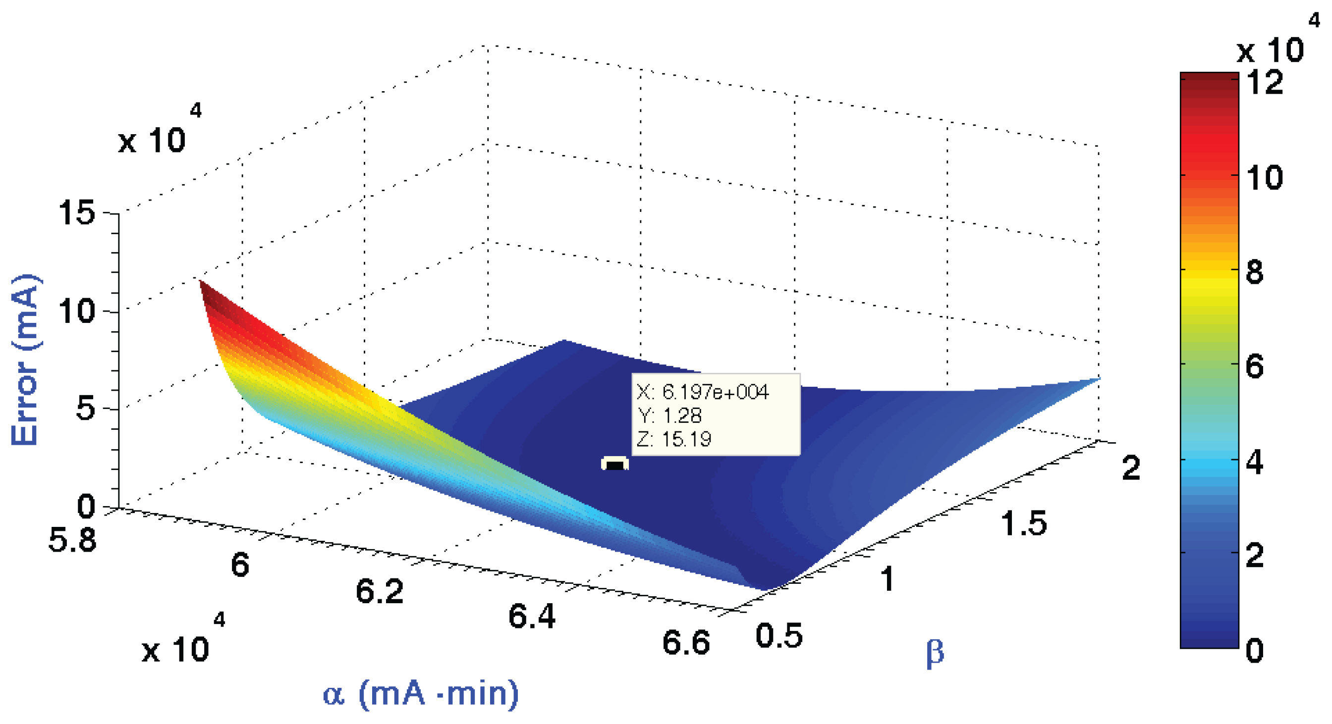
12), an error surface in Figure 10 is plotted in the range of α = 58,000 mA·min to 66,000 mA·min and β = 0.5 to 2. An optimization point is found at the location of α = 61,970 mA·min (or 1032.83 mAh) and β = 1.28.
Figure 9. Battery voltage curves of the constant discharging current tests.
Energies 09 00051 g009
Table 2. Measured runtime of the constant discharging current tests.
C-rate (C)1.00.90.80.70.60.5
Discharge time (min)54.3760.6768.7375.7591.95110.683
C-rate (C)0.40.30.20.10.02
Discharge time (min)139.03185.15278.38558.082740.93
Figure 10. Error surface to find the optimization set of the α and β parameters.
Energies 09 00051 g010
Taking the measured α and β into Equations (8) and (
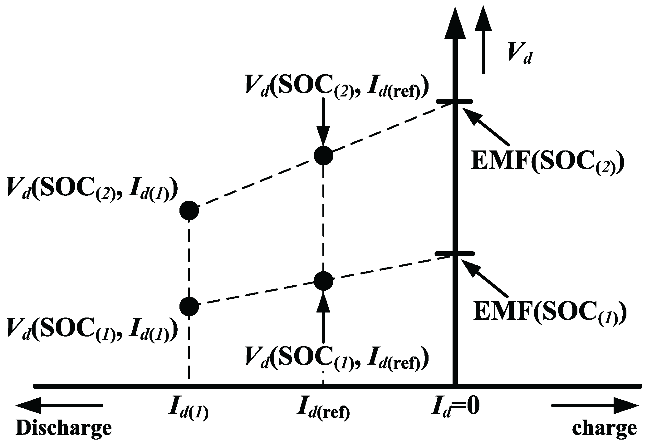
9) obtains SOCs of the 11 discharging tests for extracting parameters of the switching overpotential model, e.g., the EMF-SOC curve, R o v p -SOC curve and V o v p - I d curves. The battery voltage-SOC curves are shown in 
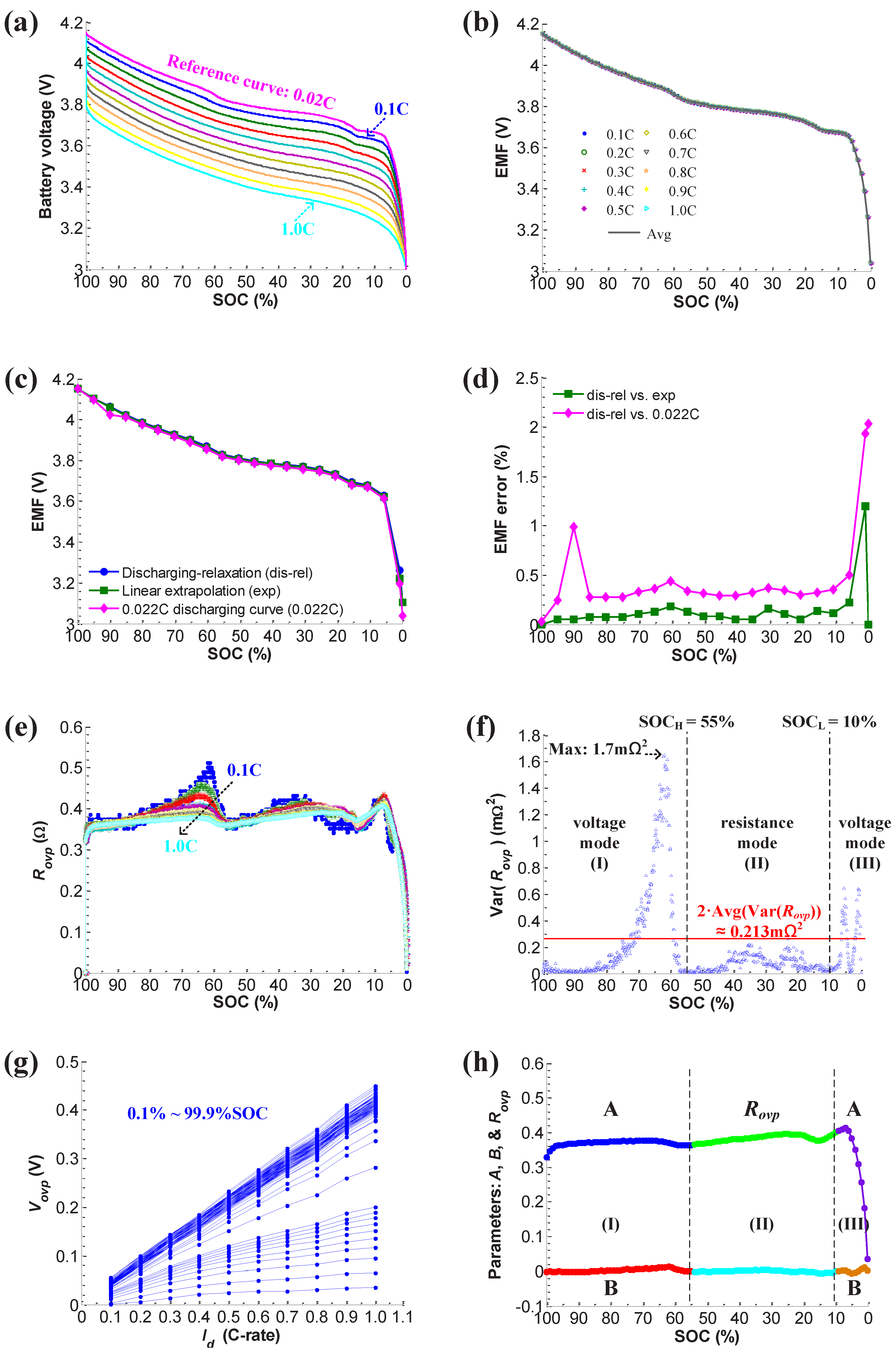
Figure 11a. The result of the 0.02 C current rate is a reference voltage curve for linearly extrapolating EMF-SOC curves. 
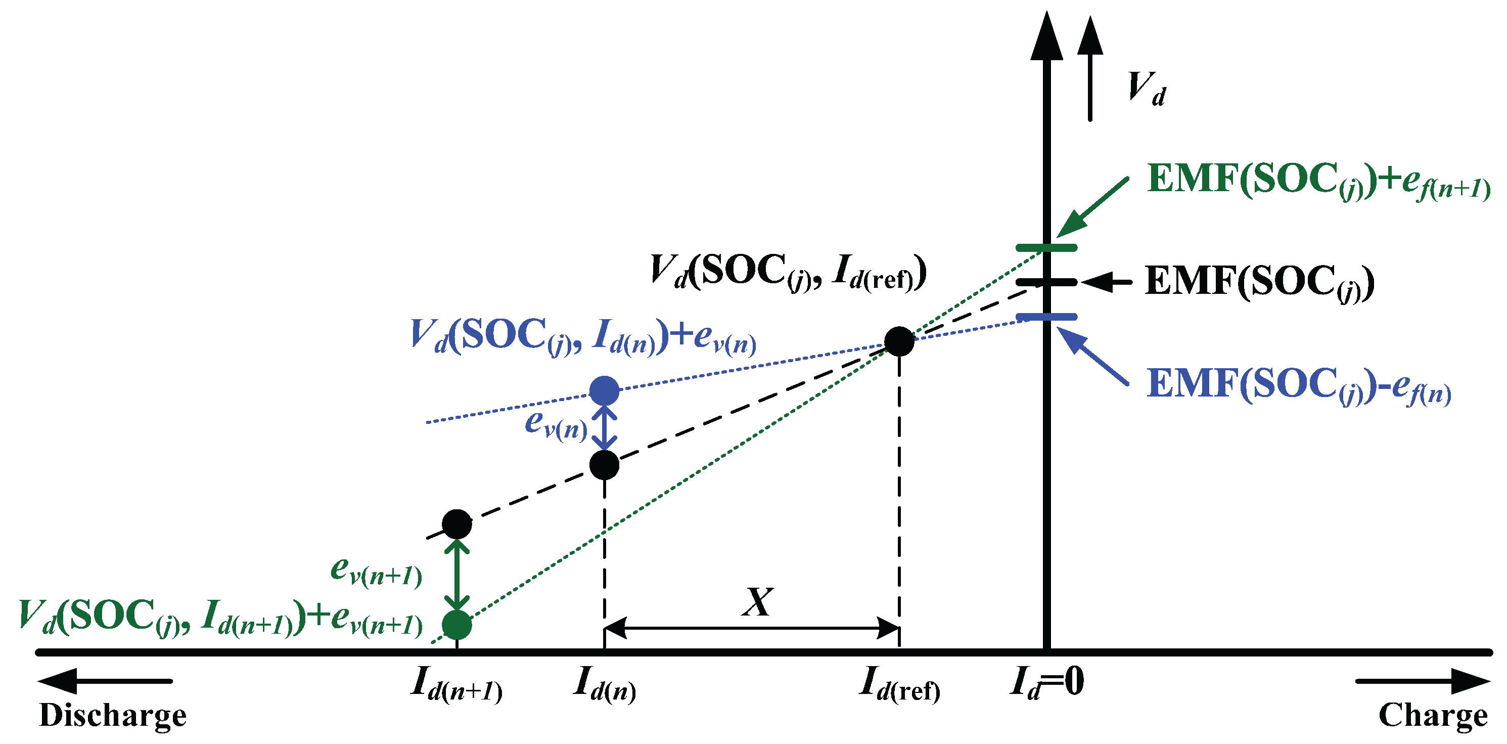
Figure 11b presents the results of EMF-SOC curves extracted from 0.1 C to 1.0 C current rates. Only the EMF-SOC curve of the 0.1 C test has a high error ratio in that the X is five in this case. Other EMF-SOC curves all present good consistency because the error ratios are less than 1%. To improve the accuracy of EMF extraction, the final EMF-SOC curve is an average result of these extracted curves. The value at each SOC point is computed by Equation (16). Figure 11c compares the voltage curves of a discharge-relaxation method, the linear extrapolation method and the 0.02 C discharging results. The discharge-relaxation method uses a 0.1 C discharging rate to measure the EMF-SOC curve. The EMF voltage is measured every 4.5% SOC. The relaxation time is one hour at each test SOC point to ensure that the battery voltage is fully recovered. The EMF errors between the discharge-relaxation curve and the extrapolation curve and between the discharge-relaxation curve and the 0.02 C discharging curve are all shown in Figure 11d. The EMF error is calculated based on Equation (26).
EMF error = EMF dis-rel V EMF dis-rel × 100 %
where EMF dis-rel is the EMF value measured by the discharge-relaxation method and V can be the voltage of the linear extrapolation method or the 0.02 C discharging result. From Figure 11d, it is obvious to observe that the error curve of the 0.02 C discharging result is higher than the error curve of the extrapolation method. The average error of the 0.02 C discharging result is about 0.5%, but the average error of the extrapolation method reduces to 0.15%. Thus, the extrapolation method is necessary for obtaining an accurate EMF-SOC curve.
Figure 11. Experimental results of parameter extraction: (a) battery voltage-SOC curves; (b) EMF-SOC curves; (c) EMF comparisons; (d) EMF errors; (e) R o v p -SOC curves; (f) variance of R o v p ; (g) V o v p - I d curves; (h) parameters: A, B and R o v p .
Energies 09 00051 g011
With battery voltage-SOC and EMF-SOC curves in hand, R o v p -SOC curves are then extracted from Equation (21). The results are shown in Figure 11e. The overpotential resistances in 10% to 90% SOC vary in 0.35 Ω to 0.52 Ω, but have large variations near 60% SOC. The variance of R o v p , or Var( R o v p ), is presented in Figure 11f. The maximum variance is 1.7 m Ω 2 and happened in the 0.1 C test result due to the low current rate. These variations are also observed in the measured voltage curves and are probably caused by the chemical reactions, such as phase transformations in lithium electrode materials [33]. The overpotential resistances have sharp changes above 90% SOC and below 10% SOC. Consequently, most of the battery models have low accuracy when they operate in the two SOC regions.
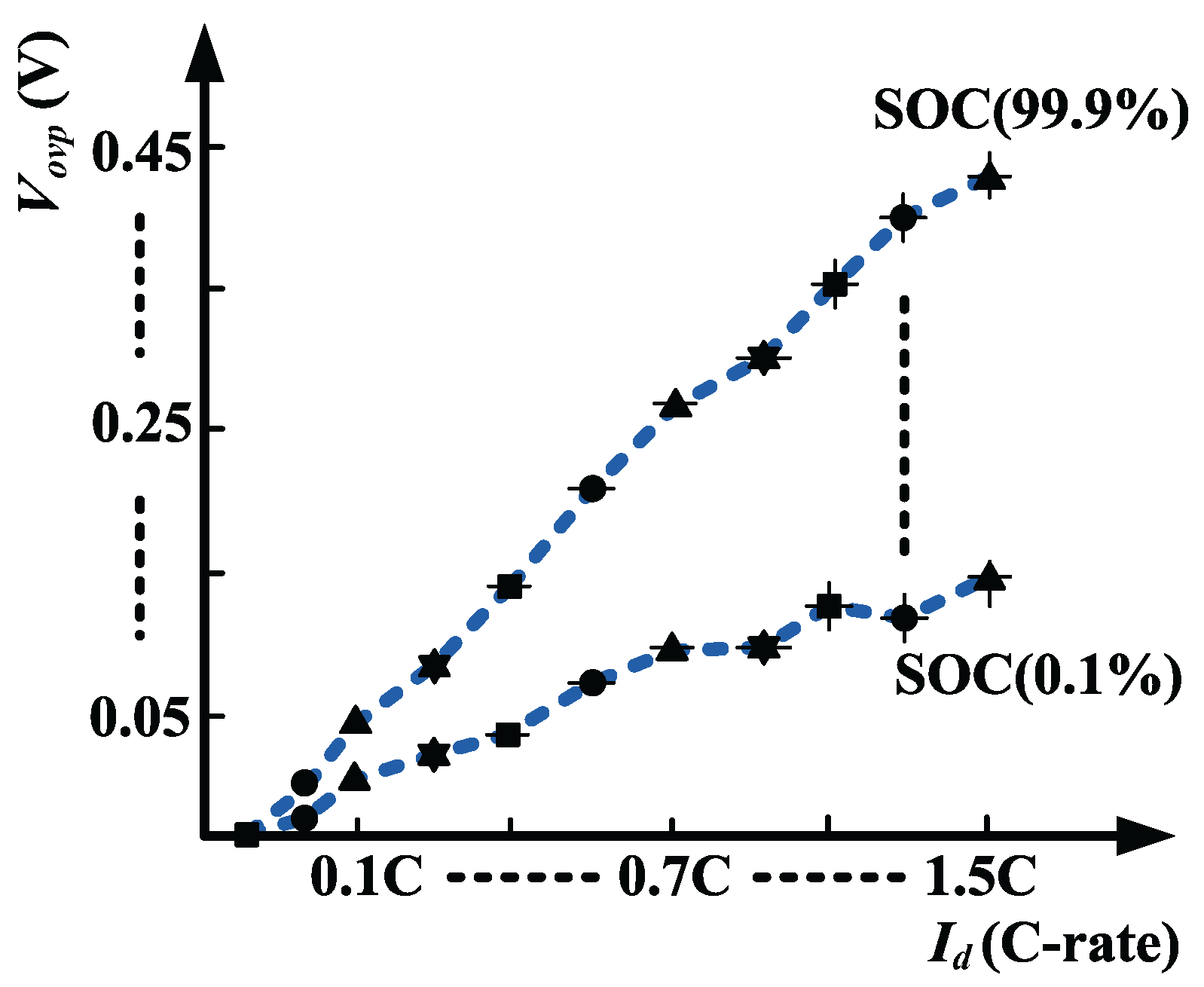
Figure 11g analyzes the overpotential voltages in the SOC range from 0.1% to 99.9%. The linear regression analysis outputs the curve-fitting results of A, B and R o v p parameters in Figure 11h. According to the average variance of R o v p , the SOC is divided into three regions. The first SOC region, or Region I, begins from 100% to 55%. This region covers the maximum variance, so the battery simulator runs in the voltage mode. The second SOC region, or Region II, begins from 54.9% to 10.1%. The second region has a stable R o v p . The average variance is less than 0.1 m Ω 2 , and the average R o v p is 0.38 Ω. In the second region, the battery simulator operates in the resistance mode. The third SOC region, or Region III, is close to empty capacity. The SOC is in the range from 10% to 0.1%. The R o v p variance increases again, so the voltage mode is a better choice. In the third region, parameter A has a sharp decrement, so the overpotential voltage would still have small prediction errors.

5.2. Results of Dynamic Load Prediction

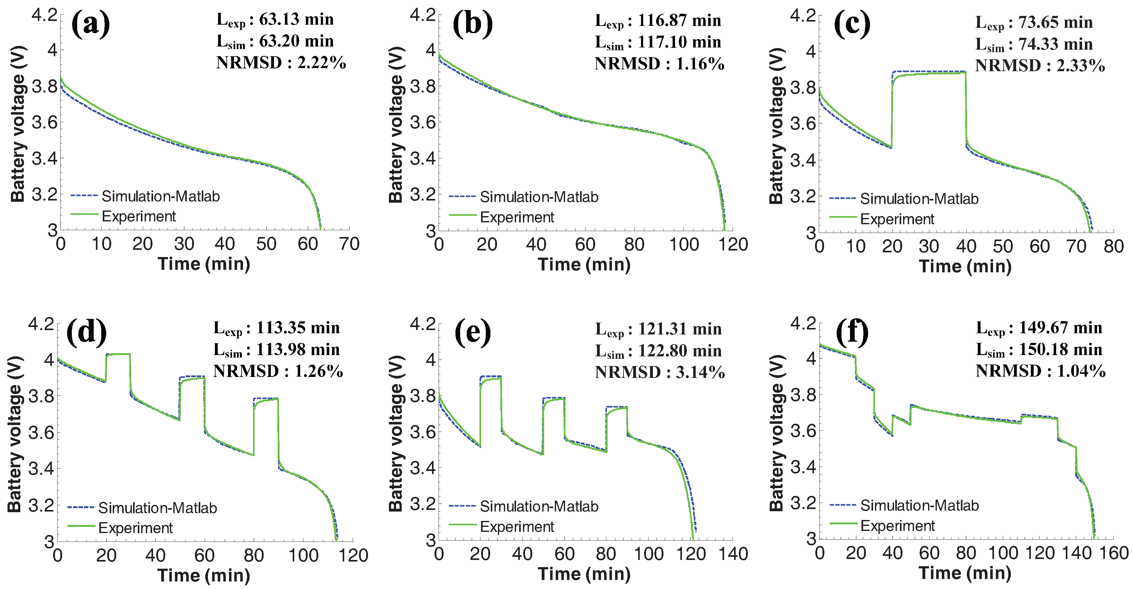
Figure 12 makes comparisons between experimental and MATLAB simulation results. For the constant current loads, the proposed simulator shows good matches in Figure 12a,b. In both cases, the rate capacity effect is reflected at the beginning of the simulations, so the terminal voltages in experiments and in simulations match well when the test cell is close to empty. The experimental runtimes of the heavy load and the light load tests are 63.13 and 116.87 min, respectively. The simulated runtime of both cases has less than 0.2% prediction errors. The normalized root mean square deviation (NRMSD), which is defined as Equation (27), recognizes the differences between simulated curves and experimental curves.
NRMSD = 1 V b , max V b , min t = 1 K ( V ^ b ( t ) V b ( t ) ) 2 K × 100 %
where K is the total measured points, V ^ b ( t ) is the simulated voltage value at time t and V b ( t ) is the experimental voltage value. The NRMSDs of the two cases are 2.2% and 1.16%. The small errors confirm that the proposed simulator is able to predict dynamic discharging behavior.
For the interrupted load, the simulation result in Figure 12c also shows a good agreement with the experimental result. The capacity recovery effect occurs during the rest period from 20 min to 40 min. After the rest period, the rate capacity effect takes place again, so the simulator successfully predicts the final runtime with a 0.92% error and dynamic behavior with 2.33% NRMSD.
For the increasing and decreasing loads, the rate capacity effect and recovery effect happen alternatively. The simulation result of the increasing load in Figure 12d predicts the runtime with a 0.54% error, while the prediction error of the decreasing load in Figure 12e slightly increases. In the overpotential voltage mode, the prediction error only grows to 1.2%. The error is mainly generated near the fully-discharged condition. A possible reason for this error would be that the low current in the finalstep lasts a long time in the low SOC region. As a result, prediction error is accumulated and increases the voltage differences between the simulation and experimental values. The NRMSD of the increasing load is 1.36%, so the proposed simulator has a good behavior prediction on the increasing load. By comparison, the NRMSD of the decreasing load is 3.14%.
Figure 12. Model validation by MATLAB simulations: (a) heavy load ( P 1 ); (b) light load ( P 2 ); (c) interrupted load ( P 3 ); (d) increasing load ( P 4 ); (e) decreasing load ( P 5 ); (f) varying load ( P 6 ).
Energies 09 00051 g012
For the varying load, there is no rest time in this profile. Besides, the current changes without any rule. The simulation result in Figure 12f validates again that the proposed simulator can accurately predict the dynamic discharging behavior and further evaluate the runtime under various discharging profiles.
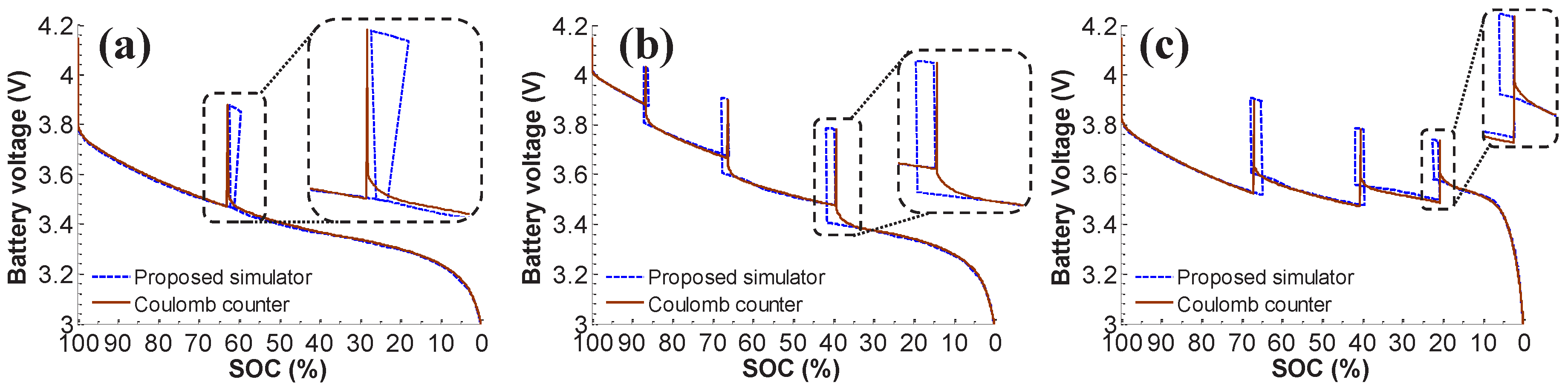
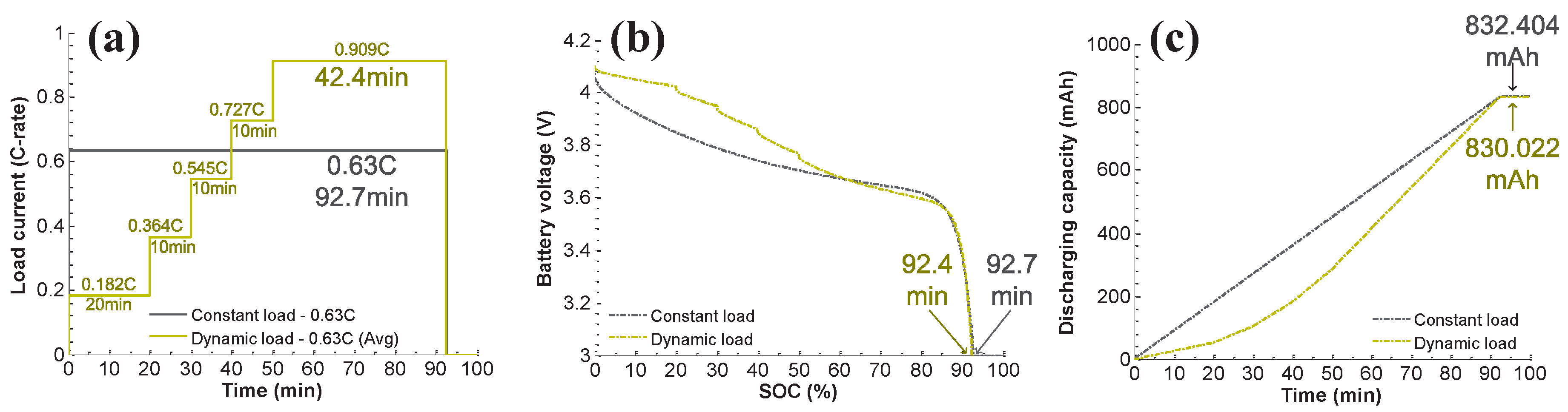
Figure 13 checks the battery voltage-SOC curves of the P 3 to P 5 profiles. In these plots, the SOCs estimated by the proposed simulator and the Coulomb counter are compared. The Coulomb counter estimates SOCs using the nominal capacity as the maximum available capacity. During the rest time, the recovering capacities are observed by the proposed battery simulator. However, the SOCs reported by the Coulomb counter do not have any change in this period of time, so this causes some runtime prediction errors.
Figure 13. Capacity recovery effects in the P 3 to P 5 profiles.
Energies 09 00051 g013
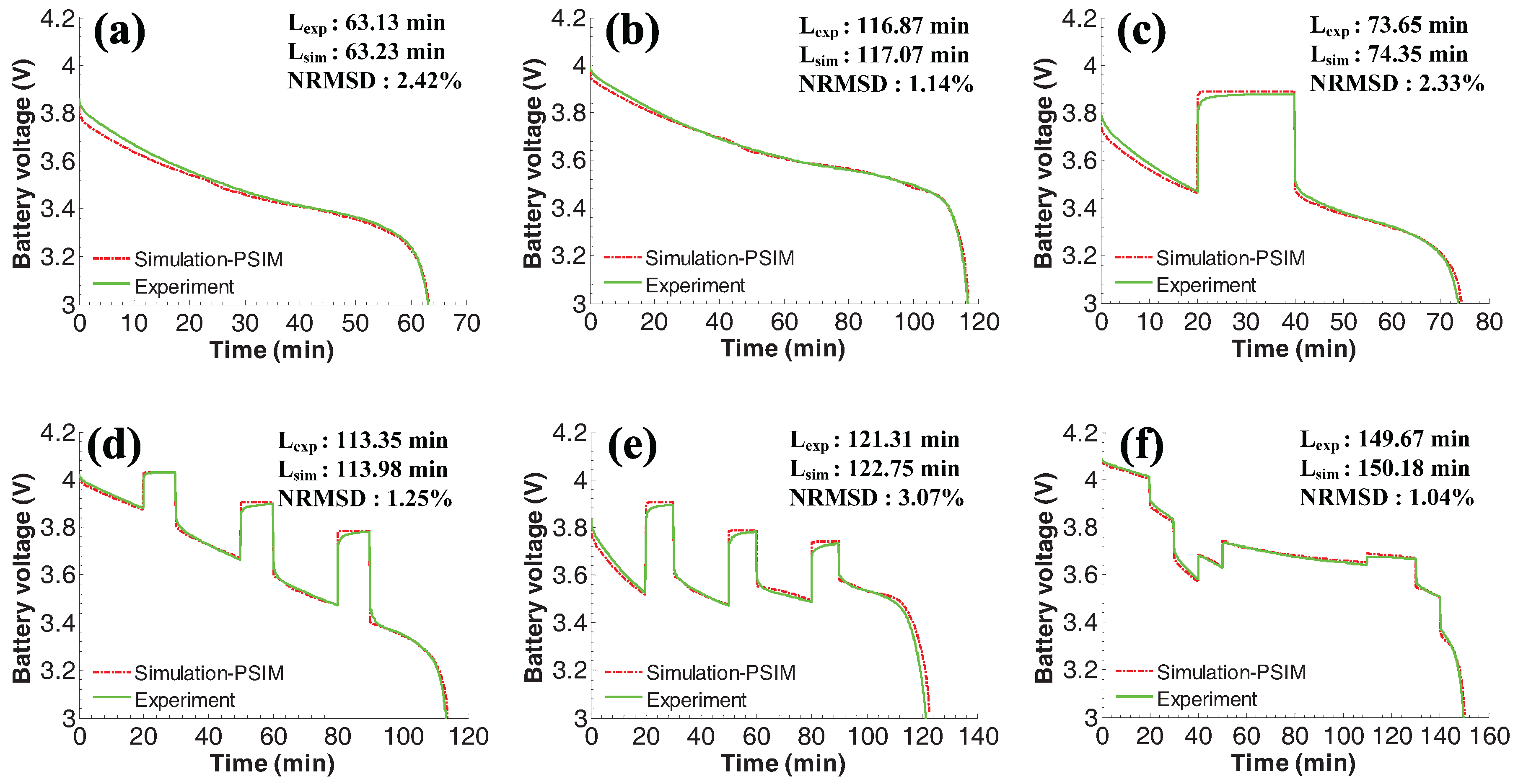
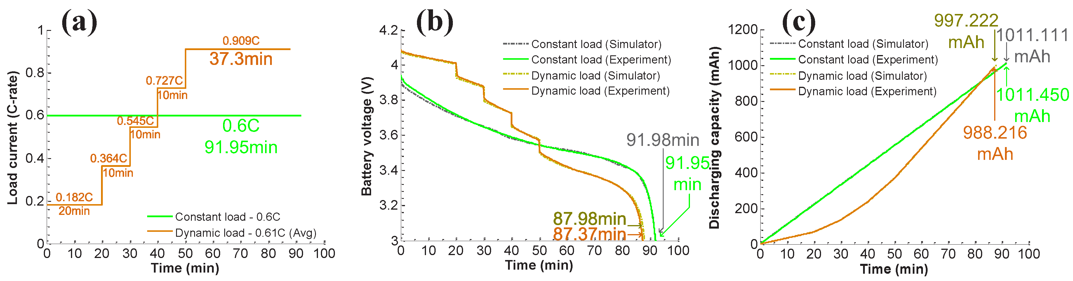
Figure 14 presents the PSIM simulations for the same profiles. The simulation comparisons are made in Table 3. The runtime and behavior errors show that there are very small differences between PSIM simulation results and MATLAB simulation results. This means that the proposed battery simulator is successfully implemented in the PSIM simulation environment for dynamic discharging behavior and runtime predictions. For both simulation tools, the simulation time of the P 1 to P 6 profiles is smaller than 5 s.
Figure 14. Model validation by PSIM simulations: (a) heavy load ( P 1 ); (b) light load ( P 2 ); (c) interrupted load ( P 3 ); (d) increasing load ( P 4 ); (e) decreasing load ( P 5 ); (f) varying load ( P 6 ).
Energies 09 00051 g014
Table 3. Simulation result comparisons. NRMSD, normalized root mean square deviation.
P 1 P 2 P 3 P 4 P 5 P 6
MATLABruntime error0.11%0.20%0.92%0.56%1.19%0.34%
behavior error (NRMSD)2.22%1.16%2.33%1.26%3.14%1.04%
PSIMruntime error0.15%0.17%0.95%0.56%1.15%0.34%
behavior error (NRMSD)2.42%1.14%2.33%1.25%3.07%1.04%
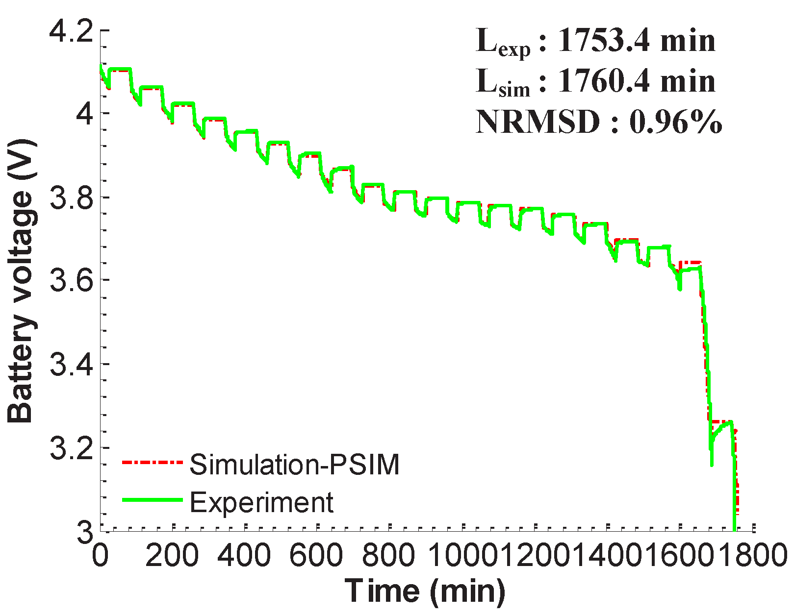
A more aggressive discharge profile to prove the predictive capability of the battery simulator is the discharge-relaxation experiment that has been applied to find the EMF-SOC curve in Figure 11c. The experiment and PSIM simulation results are shown in Figure 15. The experiment time is 1753.4 min, or 29.2 h. The runtime predicted by the proposed simulator is 1760.4 min, or 29.3 h. The runtime error is 0.4%. The behavior prediction error shows that the NRMSD is 0.96%. The PSIM simulation time of the 0.1C discharge-relaxation test is 44 s.
Figure 15. Validation of the 0.1 C discharge-relaxation test.
Energies 09 00051 g015

6. Discussion

A model comparison between the standard second-order ECM in [19] and the proposed battery simulator was conducted. To show the improvement, a dynamic current load and a constant current load were tested in simulations and experiments. Both current profiles have the same average current. The profile configuration of the dynamic current load is listed in Table 4. Although the time of 0.909 C is 100 min, the actual time is determined by the battery voltage. When the battery voltage drops to the 3.0-V cutoff voltage, simulations and experiments are terminated. The dynamic current load was tested firstly to realize in real time 0.909 C for calculating the average current rate. The constant load was then performed with this average current rate.
Table 4. Profile configuration of dynamic current load.
ProfileConfiguration: Current (Time)
Dynamic current load0.182 C (20 min)-0.364 C (10 min)-0.545 C (10 min)-0.727 C (10 min)-0.909 C (100 min)
The simulation results of the standard second-order ECM are shown in Figure 16. Table 5 summarizes the runtime and discharging capacity of the two current profiles. For the second-order ECM, the time of 0.909 C in the dynamic current load is 42.4 min, so the total discharging time is 92.4 min. The average current rate is 0.63 C. The discharging capacity is 830.022 mAh. The simulation results of the constant current load with 0.63 C show that the runtime and discharging capacity are almost the same. The runtime of the constant current load slightly increases 0.33% when it is compared to the result of the dynamic current load. The discharging capacity of the constant current load slightly increases 0.29%. The test results show that basically the two current profiles are the same for the standard ECM. However, this is not true for a real battery. In reality, the increasing current of the dynamic current profile will cause the available discharging capacity to reduce due to the rated capacity effect. The runtime will also reduce. Thus, the discharging capacity and the runtime of the dynamic current load should be lower than the results of the constant current load.
Figure 16. ECM simulation results: (a) load current; (b) battery voltage; and (c) discharging capacity.
Energies 09 00051 g016
Table 5. ECM simulation results of two different profiles with a 0.63 C average current.
ProfileRuntimeDischarging capacity
Dynamic current load92.4 min830.022 mAh
Constant current load92.7 min832.404 mAh
Growth rate(+0.33%)(+0.29%)
The same tests were conducted in experiments with the Nokia BL-5C polymer Li-ion battery cell and simulations with the proposed battery simulator. The experimental data and simulation results are shown in Figure 17. Two current profiles for testing in experiments are shown in Figure 17a. Figure 17b shows not only experimental battery voltages of the two current profiles, but also the simulated battery voltages of the proposed battery simulator for validations. Figure 17c shows the discharging capacities of the two current loads. Table 6 summarizes the runtime and discharging capacity. Experimental data show that the time of 0.909 C in the dynamic current load lasts only 37.3 min. The total experimental time of the dynamic current load reduces to 87.3 min, and the average current is 0.61 C. Comparing to the 0.6 C constant current, which was performed in model parameter extraction tests to obtain the α and β parameters in Section 4, the runtime is 91.95 min. This result is much higher than the runtime of the dynamic current load.
Figure 17. Experimental data and simulation results of the proposed battery simulator: (a) load current; (b) battery voltage; and (c) discharging capacity.
Energies 09 00051 g017
Table 6. Experimental data and simulation results of the proposed battery simulator.
ProfileRuntimeDischarging Capacity
ExperimentSimulatorExperimentSimulator
Dynamic current load87.37 min87.98 min988.216 mAh997.222 mAh
Constant current load91.95 min91.98 min1011.450 mAh1011.111 mAh
Growth rate(+5.24%)(+4.55%)(+2.35%)(+1.39%)
The nonlinear capacity effects can be clearly observed from the experimental data and simulation results. Due to the increasing load current, the rated capacity effect causes the available discharging charge of the dynamic current load to reduce, so the runtime is less than the time of the constant current load. The experimental data show that the runtime and the discharging capacity of the constant current load increase 5.24% and 2.35%, respectively. The simulation results show that the runtime and the discharging capacity of the constant current load increase 4.55% and 1.39%. If the average current of the current profile rises, the runtime differences between a dynamic current load and a constant current load will also increase. This example definitely illustrates the superiority of the proposed battery simulator over the standard ECM. The proposed battery simulator has the capability of reflecting the nonlinear capacity effects in a dynamic discharging current load. However, the standard ECM cannot make the difference between a constant current load and a dynamic current load with the same average current rate. Thus, the standard ECM cannot reflect the runtime and discharging capacity reductions under a dynamic current load.

7. Conclusions

This paper has presented a new battery simulator, which can predict battery dynamic behavior and runtime in existing electronic simulation environments. A hybrid battery model that combines the diffusion model for enhancing the ability to capture the nonlinear capacity effects and a switching overpotential model for simulating the battery terminal voltage have been presented. The linear extrapolation technique has also been introduced to extract the parameters of the two models. A Nokia BL-5C polymer Li-ion battery cell with the 1020 mAh nominal capacity has been used to validate the proposed simulator. In total, 11 constant discharging current, 0.02 C and 0.1 C to 1.0 C, have been tested for extracting parameters, including α and β for the diffusion model and EMF, overpotential resistance and voltage for the switching overpotential model. The six predefined profiles have been tested in the experiments to check the estimation performances of the simulator under a heavy load, a light load, an interrupted load, increasing and decreasing loads and a varying load. The same profiles have also been tested in MATLAB and PSIM simulations. The results confirm the usefulness and accuracy of the simulator to predict dynamic discharging behavior and battery runtime in electronic design environments for co-simulating and co-designing with electrical circuits and systems.

Acknowledgments

The authors would like to give thanks for the research grant (MOST 102-2221-E-009-145) from the Ministry of Science and Technology (MOST), Taipei, Taiwan.

Author Contributions

Lan-Rong Dung developed the essential ideal of the proposed battery simulator, designed some parts of the experiments and gave some suggestions. Chien-Hua She and Ming-Han Lee carried out the experiments and built the simulator in MATLAB and PSIM. Lan-Rong Dung and Hsiang-Fu Yuan checked the experiment and simulation results. Hsiang-Fu Yuan and Jieh-Hwang Yen wrote the manuscript. The final review and revision were done by Lan-Rong Dung and Hsiang-Fu Yuan.

Conflicts of Interest

The authors declare no conflict of interest.

References

  1. Gao, J.; Zhang, Y.; He, H. A real-time joint estimator for model parameters and state of charge of lithium-ion batteries in electric vehicles. Energies 2015, 8, 8594–8612. [Google Scholar] [CrossRef]
  2. Xia, B.; Wang, H.; Tian, Y.; Wang, M.; Sun, W.; Xu, Z. State of charge estimation of lithium-ion batteries using an adaptive cubature kalman filter. Energies 2015, 8, 5916–5936. [Google Scholar] [CrossRef]
  3. Uddin, K.; Picarelli, A.; Lyness, C.; Taylor, N.; Marco, J. An acausal Li-ion battery pack model for automotive applications. Energies 2014, 7, 5675–5700. [Google Scholar] [CrossRef]
  4. Sepasi, S.; Roose, L.R.; Matsuura, M.M. Extended kalman filter with a fuzzy method for accurate battery pack state of charge estimation. Energies 2015, 8, 5217–5233. [Google Scholar] [CrossRef]
  5. Lee, J.; Yi, J.; Shin, C.B.; Yu, S.H.; Cho, W.I. Modeling the effects of the cathode composition of a lithium iron phosphate battery on the discharge behavior. Energies 2013, 6, 5597–5608. [Google Scholar] [CrossRef]
  6. Dees, D.W.; Battaglia, V.S.; Bélanger, A. Electrochemical modeling of lithium polymer batteries. J. Power Sources 2002, 110, 310–320. [Google Scholar] [CrossRef]
  7. Newman, J.; Thomas, K.E.; Hafezi, H.; Wheeler, D.R. Modeling of lithium-ion batteries. J. Power Sources 2003, 119–121, 838–843. [Google Scholar] [CrossRef]
  8. Gomadam, P.M.; Weidner, J.W.; Dougal, R.A.; White, R.E. Mathematical modeling of lithium-ion and nickel battery systems. J. Power Sources 2002, 110, 267–284. [Google Scholar] [CrossRef]
  9. Klein, R.; Chaturvedi, N.; Christensen, J.; Ahmed, J.; Findeisen, R.; Kojic, A. Electrochemical model based observer design for a lithium-ion battery. IEEE Trans. Control Syst. Technol. 2013, 21, 289–301. [Google Scholar] [CrossRef]
  10. Ahmed, R.; El Sayed, M.; Arasaratnam, I.; Tjong, J.; Habibi, S. Reduced-order electrochemical model parameters identification and state of charge estimation for healthy and aged Li-ion batteries-Part II: Aged battery model and state of charge estimation. IEEE J. Emerg. Sel. Top. Power Electron. 2014, 2, 678–690. [Google Scholar] [CrossRef]
  11. Pedram, M.; Wu, Q. Design considerations for battery-powered electronics. In Proceedings of the 36th Annual ACM/IEEE Design Automation Conference, New Orleans, LA, USA, 21–25 June 1999; pp. 861–866.
  12. Chiasserini, C.; Rao, R. Energy efficient battery management. IEEE J. Sel. Areas Commun. 2001, 19, 1235–1245. [Google Scholar] [CrossRef]
  13. Linden, D.; Reddy, T.B. Handbook of Batteries, 3rd ed.; McGraw-Hill: New York, NY, USA, 2002. [Google Scholar]
  14. Manwell, J.F.; McGowan, J.G. Lead acid battery storage model for hybrid energy systems. Sol. Energy 1993, 50, 399–405. [Google Scholar] [CrossRef]
  15. Rakhmatov, D.; Vrudhula, S.; Wallach, D. A model for battery lifetime analysis for organizing applications on a pocket computer. IEEE Trans. VLSI Syst. 2003, 11, 1019–1030. [Google Scholar] [CrossRef]
  16. Rong, P.; Pedram, M. An analytical model for predicting the remaining battery capacity of lithium-ion batteries. IEEE Trans. VLSI Syst. 2006, 14, 441–451. [Google Scholar] [CrossRef]
  17. Agarwal, V.; Uthaichana, K.; DeCarlo, R.; Tsoukalas, L. Development and validation of a battery modelu useful for discharging and charging power control and lifetime estimation. IEEE Trans. Energy Convers. 2010, 25, 821–835. [Google Scholar] [CrossRef]
  18. Schweighofer, B.; Raab, K.; Brasseur, G. Modeling of high power automotive batteries by the use of an automated test system. IEEE Trans. Instrum. Meas. 2003, 52, 1087–1091. [Google Scholar] [CrossRef]
  19. Chen, M.; Rincon-Mora, G. Accurate electrical battery model capable of predicting runtime and I-V performance. IEEE Trans. Energy Convers. 2006, 21, 504–511. [Google Scholar] [CrossRef]
  20. Szumanowski, A.; Chang, Y. Battery management system based on battery nonlinear dynamics modeling. IEEE Trans. Veh. Technol. 2008, 57, 1425–1432. [Google Scholar] [CrossRef]
  21. Hu, X.; Li, S.; Peng, H. A comparative study of equivalent circuit models for Li-ion batteries. J. Power Sources 2012, 198, 359–367. [Google Scholar] [CrossRef]
  22. Thirugnanam, K.; Ezhil Reena, J.; Singh, M.; Kumar, P. Mathematical modeling of Li-ion battery using genetic algorithm approach for V2G applications. IEEE Trans. Energy Convers. 2014, 29, 332–343. [Google Scholar]
  23. Sánchez, L.; Blanco, C.; Antón, J.; García, V.; González, M.; Viera, J. A variable effective capacity model for LiFePO4 traction batteries using computational intelligence techniques. IEEE Trans. Ind. Electron. 2015, 62, 555–563. [Google Scholar] [CrossRef]
  24. Yang, H.C.; Dung, L.R. An accurate Lithium-ion battery gas gauge using two-phase STC modeling. In Proceedings of the IEEE 16th International Symposium on Industrial Electronics (ISIE), Vigo, Spain, 4–7 June 2007; pp. 866–871.
  25. Kim, T.; Qiao, W. A hybrid battery model capable of capturing dynamic circuit characteristics and nonlinear capacity effects. IEEE Trans. Energy Convers. 2011, 26, 1172–1180. [Google Scholar] [CrossRef]
  26. Zhang, J.; Ci, S.; Sharif, H.; Alahmad, M. An enhanced circuit-based model for single-cell battery. In Proceedings of the 25th Annual IEEE Applied Power Electronics Conference and Exposition (APEC), Palm Springs, CA, USA, 21–25 February 2010; pp. 672–675.
  27. Zhang, J.; Ci, S.; Sharif, H.; Alahmad, M. Modeling discharge behavior of multicell battery. IEEE Trans. Energy Convers. 2010, 25, 1133–1141. [Google Scholar] [CrossRef]
  28. Hentunen, A.; Lehmuspelto, T.; Suomela, J. Time-domain parameter extraction method for Thévenin-equivalent circuit battery models. IEEE Trans. Energy Convers. 2014, 29, 558–566. [Google Scholar] [CrossRef]
  29. Yao, L.W.; Aziz, J.; Kong, P.Y.; Idris, N. Modeling of lithium-ion battery using MATLAB/simulink. In Proceedings of the 39th Annual Conference of the IEEE Industrial Electronics Society, Vienna, Austria, 10–13 November 2013; pp. 1729–1734.
  30. Abu-Sharkh, S.; Doerffel, D. Rapid test and non-linear model characterisation of solid-state lithium-ion batteries. J. Power Sources 2004, 130, 266–274. [Google Scholar] [CrossRef]
  31. Kim, J.; Seo, G.S.; Chun, C.; Cho, B.H.; Lee, S. OCV hysteresis effect-based SOC estimation in extended Kalman filter algorithm for a LiFePO4/C cell. In Proceedings of the 2012 IEEE International Electric Vehicle Conference (IEVC), Greenville, SC, USA, 4–8 March 2012; pp. 1–5.
  32. Baronti, F.; Femia, N.; Saletti, R.; Visone, C.; Zamboni, W. Hysteresis modeling in Li-ion batteries. IEEE Trans. Magn. 2014, 50, 1–4. [Google Scholar] [CrossRef]
  33. Guena, T.; Leblanc, P. How depth of discharge affects the cycle life of Lithium-Metal-Polymer batteries. In Proceedings of the 28th Annual International Telecommunications Energy Conference, Providence, RI, USA, 10–14 September 2006; pp. 1–8.

