2.2. Fast Predictive Peak Current Saturation Method
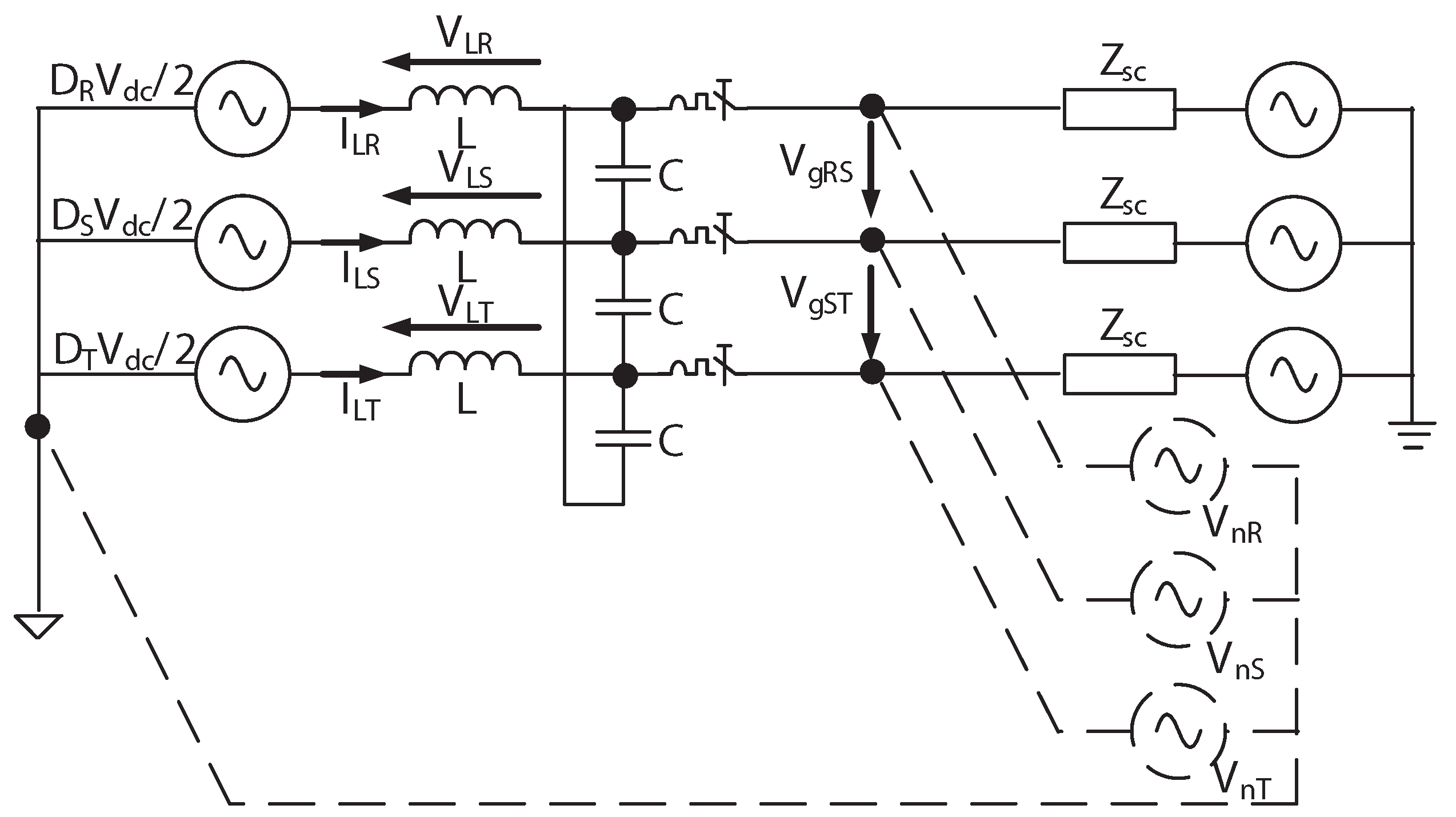
Figure 3 shows a simplified single-line model of the converter as an ideal controlled voltage source. This model has been widely presented in the literature [
22]. The converter output line-to-line voltage (
VgRS,
VgST) is defined by an impedance (
Zsc) and a grid voltage source. The measured voltage could be used to build up an equivalent voltage source model (
VnR,
VnS,
VnT) connected to the virtual neutral point of the converter model (noted by the dashed lines in
Figure 3).
Equation (
1) shows the relationship of the inductor voltage (
VL) with the voltage source model of
Figure 3 and with the differential equation of an inductor:
where
Vdc is the DC-link voltage,
Vn is the grid voltage,
D is the DG duty control signal in the range of [−1, 1],
L is the inductive value of the filter value and
IL is the current across the inductance. Since the controller is executed periodically at a fixed frequency
Fs, Equation (
1) could be discretized, and
D would be given by Equation (
2):
Figure 3.
Simplified inverter voltage source model.
Figure 3.
Simplified inverter voltage source model.
Equation (
2) gives the relationship between
IL time evolution and the control signal value. Consequently, the current measurement on the next step control could be predicted. Imposing a control law restriction with a maximum current threshold
IFPPCS, Equation (
3) sets a theoretical maximum control signal:
where
,
and
are the maximum duty allowed control signals for the defined
IFPPCS in each phase and
,
and
are the measured currents of the three phases at the
k instant.
2.3. Duty Signal Updating Improvement Method
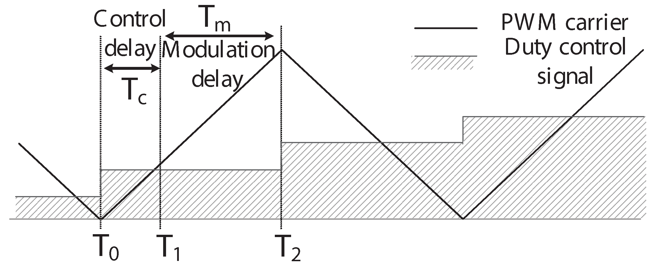
Typically, PWM techniques update only their control signals in the valleys and peaks of the triangular carrier,
T0 and
T2 respectively (see
Figure 4), guaranteeing non-desirable firing, the switching frequency remaining constant and avoiding extra power losses [
23].
Figure 4 shows a typical delay added in a power converter controller. If the control processor needs the computational time (
Tc) since the last sampling time (
T0), then an additional delay of
Tm will be inserted before the action will be executed, because the control signal can only be updated in the peaks and the valleys. The proposed technique updates the control signal at
T1 with some restrictions. Then, only
Tc delay happens, and the peak current under faulty conditions will drop.
Figure 4.
Typical delay added in a power converter controller. The measures are taken at T0, but Tc is needed to calculate the next control signal. Finally, the control signal is updated and applied at T2. Pulse width modulation: PWM.
Figure 4.
Typical delay added in a power converter controller. The measures are taken at T0, but Tc is needed to calculate the next control signal. Finally, the control signal is updated and applied at T2. Pulse width modulation: PWM.
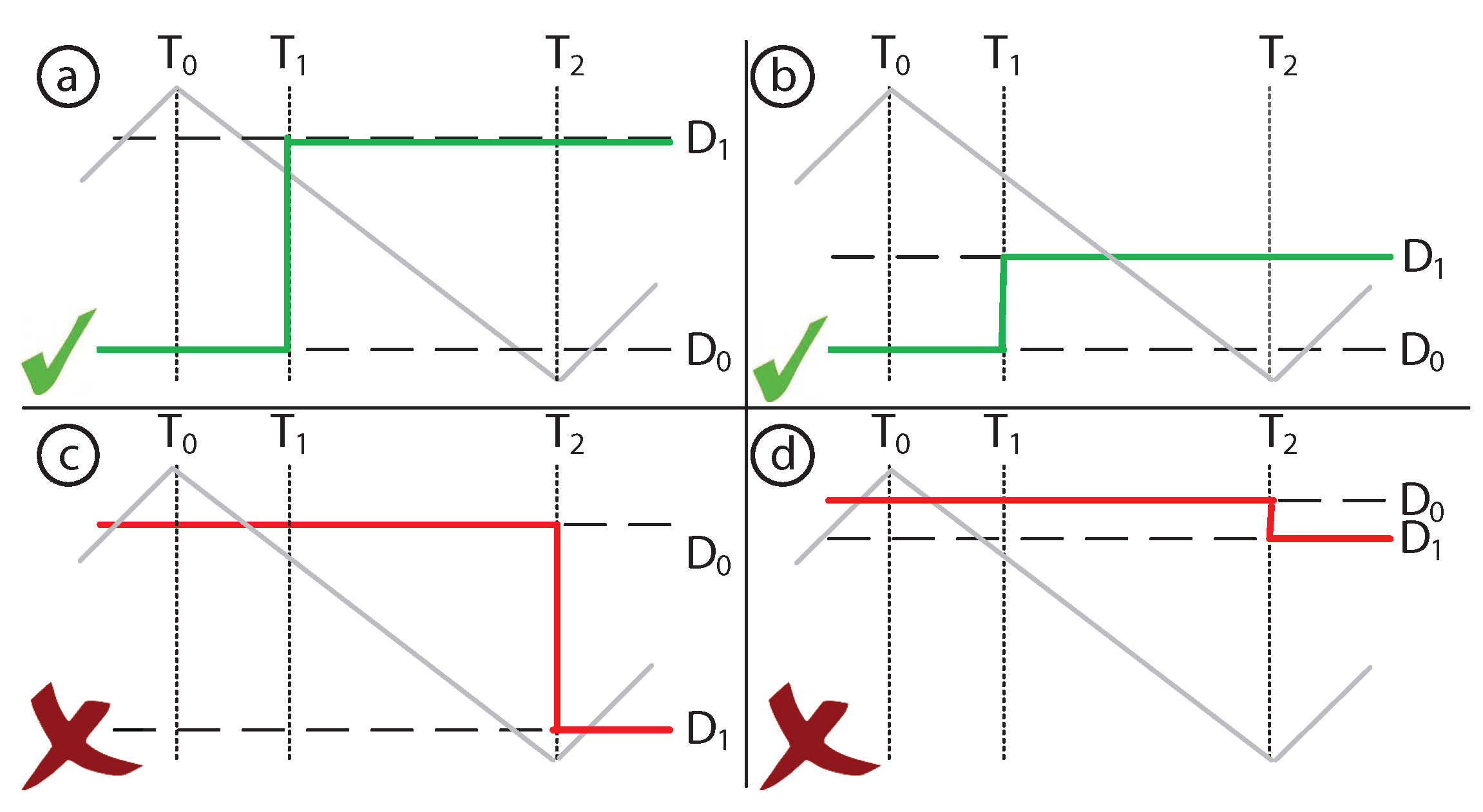
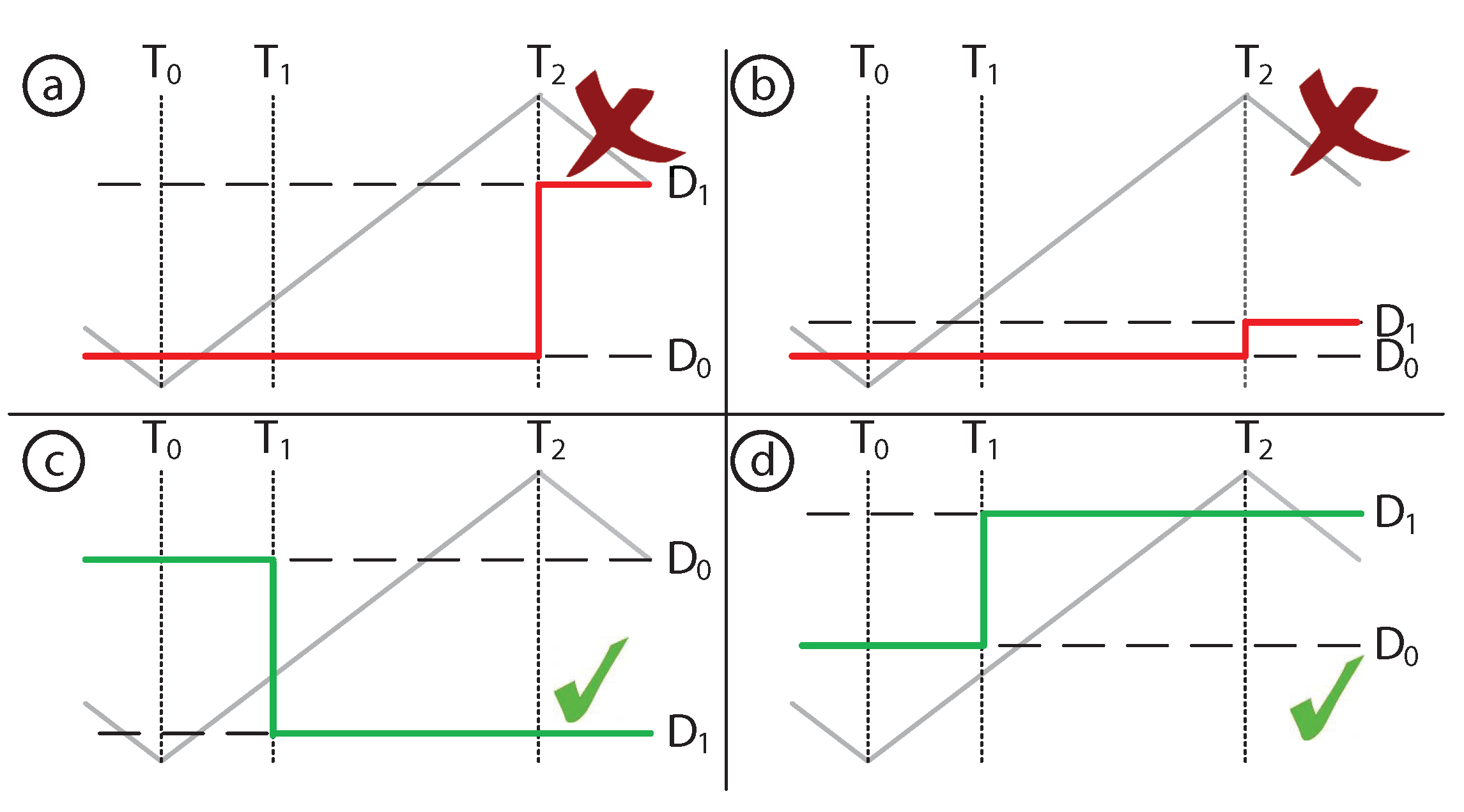
As an example,
Figure 5 shows all four possible cases in the up-slope PWM carrier semi-cycle, but similar cases could be exposed in the down-slope semi-cycle. On the one hand, during the up-slope, if the previous control signal (
D0) is greater than the triangular carrier value at
T1, no extra transition is guaranteed, and the new control signal (
D1) could be updated without any additional switching in the semi-cycle (Cases c and d in
Figure 5). On the other hand, if
D0 is lower than the triangular carrier at
T1, at least three transitions may occur if
D1 is updated at
T1: the first one belongs to the
D0 level; a second transition happens at
T1; and a third transition will happen at the
D1 level. Consequently, the control signal will be updated in the next valley or peak to avoid extra switching (Case a in
Figure 5). Finally, Case b does not produce any extra-switching, but neither modifies the control output.
Figure 5.
All four possible duty updating cases in the rising PWM semi-cycle. The control signal could be updated at T1 in Cases c and d, but must be updated at T2 in Cases a and b.
Figure 5.
All four possible duty updating cases in the rising PWM semi-cycle. The control signal could be updated at T1 in Cases c and d, but must be updated at T2 in Cases a and b.
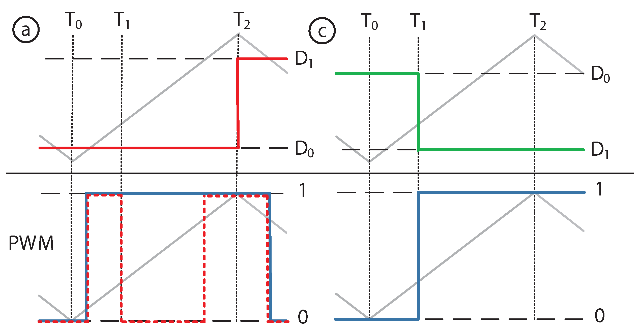
Graphically,
Figure 6 shows an example of PWM signals generated in Cases a and c. In Case c, the duty signal is updated (blue line) without producing extra switching, reducing the on state of the semiconductor. However, in Case a, the control signal must be updated in
T2 (solid blue line); otherwise, two switching events will happen (dotted red line).
Figure 6.
PWM signals generated with Cases a and c of the rising PWM semi-cycle. The red dotted line points out possible malfunctioning with two switchings in the same semi-cycle if the proposed rule is not applied. The blue line points out PWM signals generated with the duty signal updating improvement (DSUI) method.
Following the same steps, along the modulation down-slope cycle, if
D0 is lower than the modulation value at
T1, the control signal could be updated without any change in the switching frequency.
Figure 7 shows all four possible cases on the down-slope semi-cycle.
Figure 7.
All four possible duty updating cases in the falling PWM semi-cycle. The control signal could be updated at T1 in Cases a and b, but must be updated at T2 in Cases c and d.
Figure 7.
All four possible duty updating cases in the falling PWM semi-cycle. The control signal could be updated at T1 in Cases a and b, but must be updated at T2 in Cases c and d.
Fortunately, not all cases are relevant with respect to current faults. Therefore, a study could be made to determine the effectiveness of the improvement in these special cases. There are two fault conditions: a positive and a negative over-current peak. From here, the up-slope case will be analyzed, but a similar reasoning could be done for the down-slope semi-cycle.
According to Equation (
2), at instant
k = 1, the worst over-current peak (
) would happen if the current peak fault was add up over the maximum current value modulated. Consequently,
D0 is expected to be positive and big enough. In addition, if a dangerous peak current happened, the controller would have to drop
IL to a safety region. According to Equation (
2), to take down
,
D1 will be very low. Therefore, if a positive over-current peak happens, Case c of
Figure 5 is expected. As previously mentioned, this is one of the allowed cases to refresh the control signal, so the over-current peak will be reduced.
A similar reasoning could be made with a negative over-current fault. On the one hand, now,
D0 is expected to be negative and big enough. On the other hand, from Equation (
2), the
D1 expected value will be very high. Consequently, if a negative over-current peak happens, Case a or d of
Figure 5 is expected. If Case d happens, the control signal will be updated, and the over-current peak will be reduced. Unfortunately, if Case a happens, the method will not act in this semi-cycle.
Figure 5 points out that
Tc influences the effectiveness of the method. If
Tc is forced to zero, all control steps will be in the c and d cases, so it is important to have a small delay
Tc to short the measured peak current in most situations.
Finally, one more action could be performed to reduce the over-current peak. A fault happening in semi-cycle k will be measured at the beginning of the next semi-cycle k + 1, and the control action will be placed at T1 in the best case or at the beginning of k + 2 in the worst case. Therefore, the maximum delay could be 2Ts or Ts + Tc.
If
Tc is relatively short, a new control step could be done at the middle of the semi-cycle. This control signal will be applied with the same rules as the others, so in a general way, it will be placed at the final part of the semi-cycle. In this case, if a fault happens at the middle of the semi-cycle
k′, it will be measured at the beginning of the next control step
k′ + 1, and the control action will be placed at
T1 in the best case or at the beginning of
k′ + 2 in the worst case. Therefore, the maximum delay could be
Ts or 0.5 ·
Ts +
Tc. Assuming
VL constant in a short period of time during the fault condition:
where Δ
IL is the expected increment on the peak current induced by the fault and
Tdelay is the time necessary to control the fault. Therefore, according to Equation (
4), the peak current will be reduced in:
where
PI is the proportion of the peak current reduced with the improvement (between 50% and 75%).


