
Single-Source Multi-Battery Solar Charger: Analysis and Stability Issues


Abstract
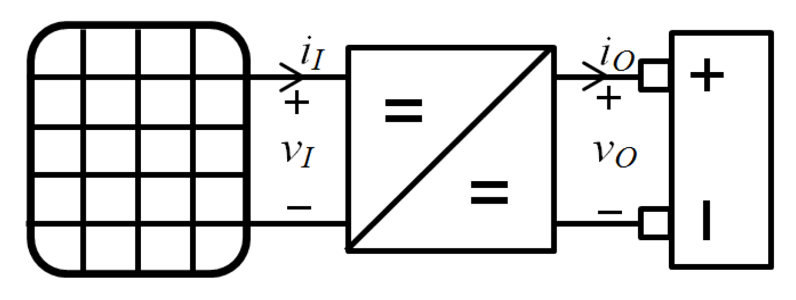
:1. Introduction
2. Single Battery Case

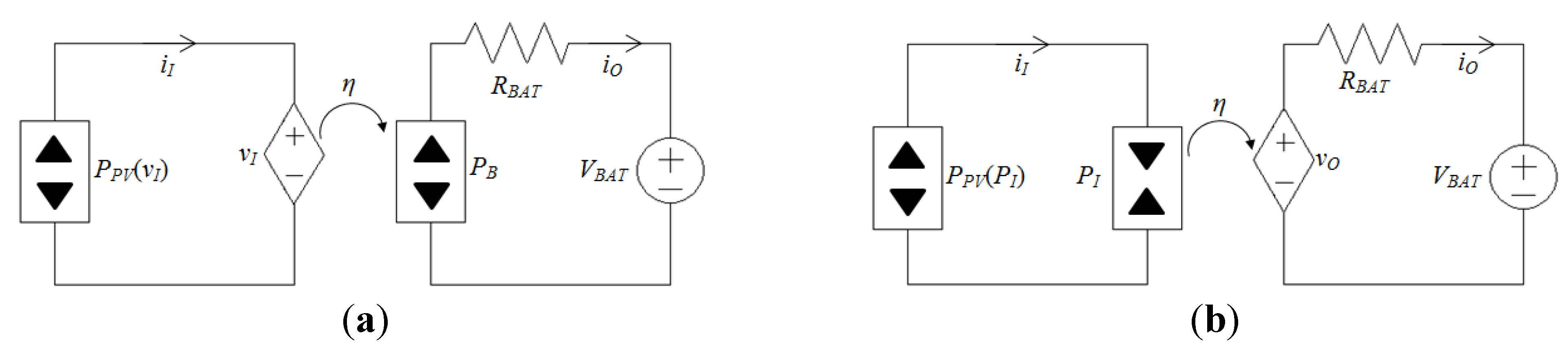
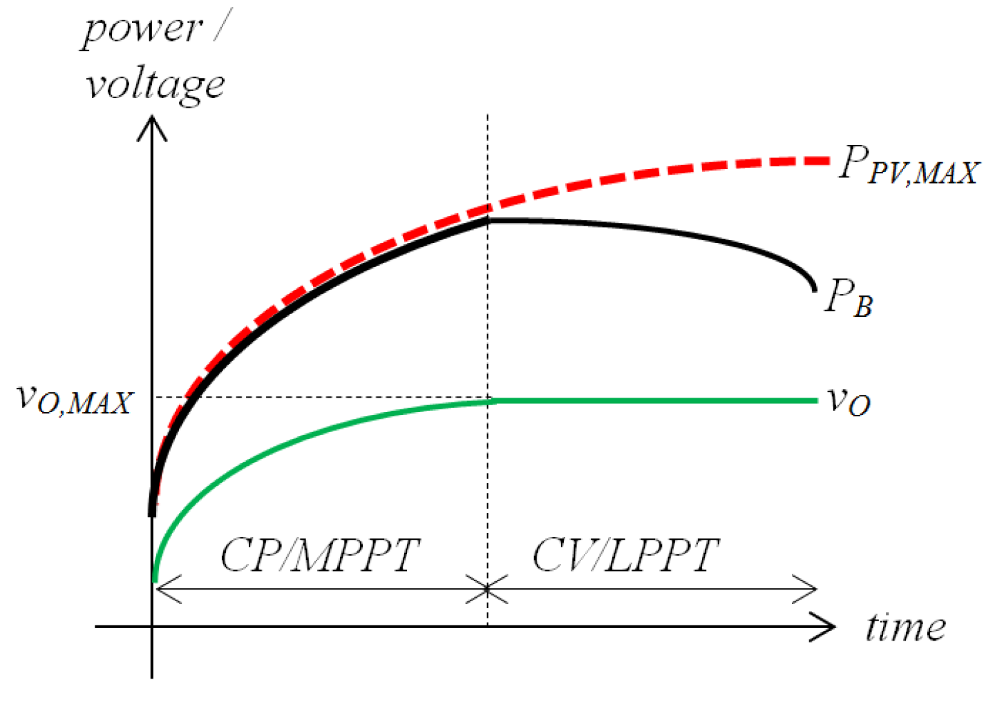
2.1. Operating Modes


2.1.1. Static Instability
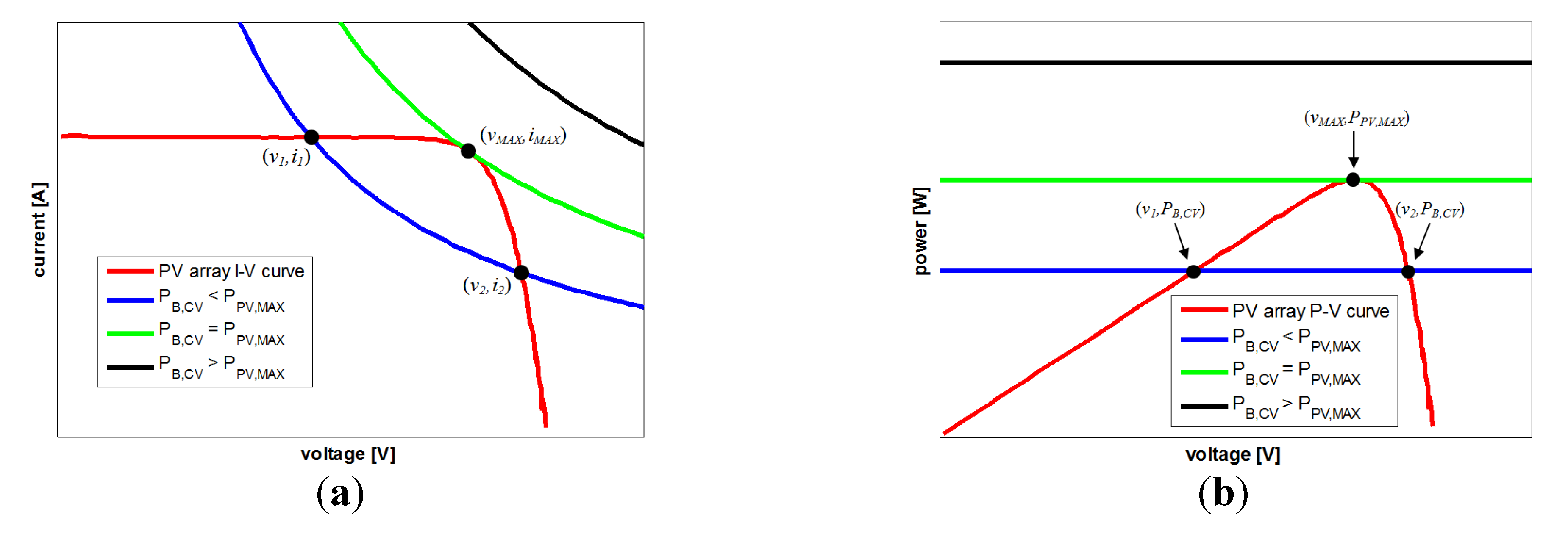
2.1.2. Operation Point Loss

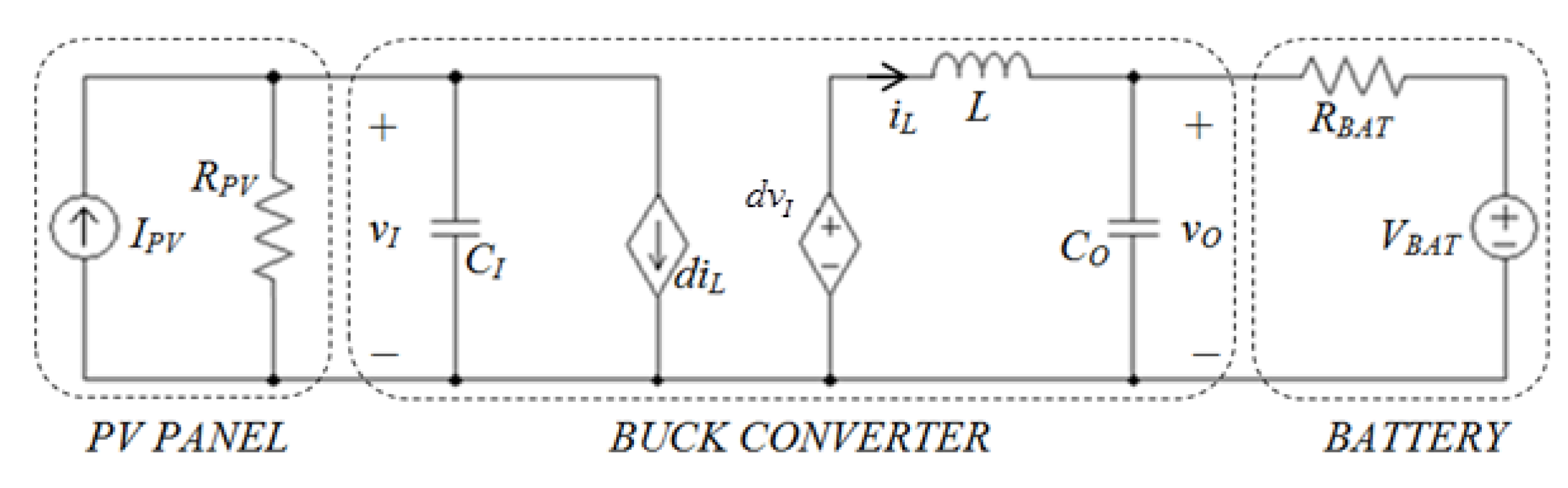
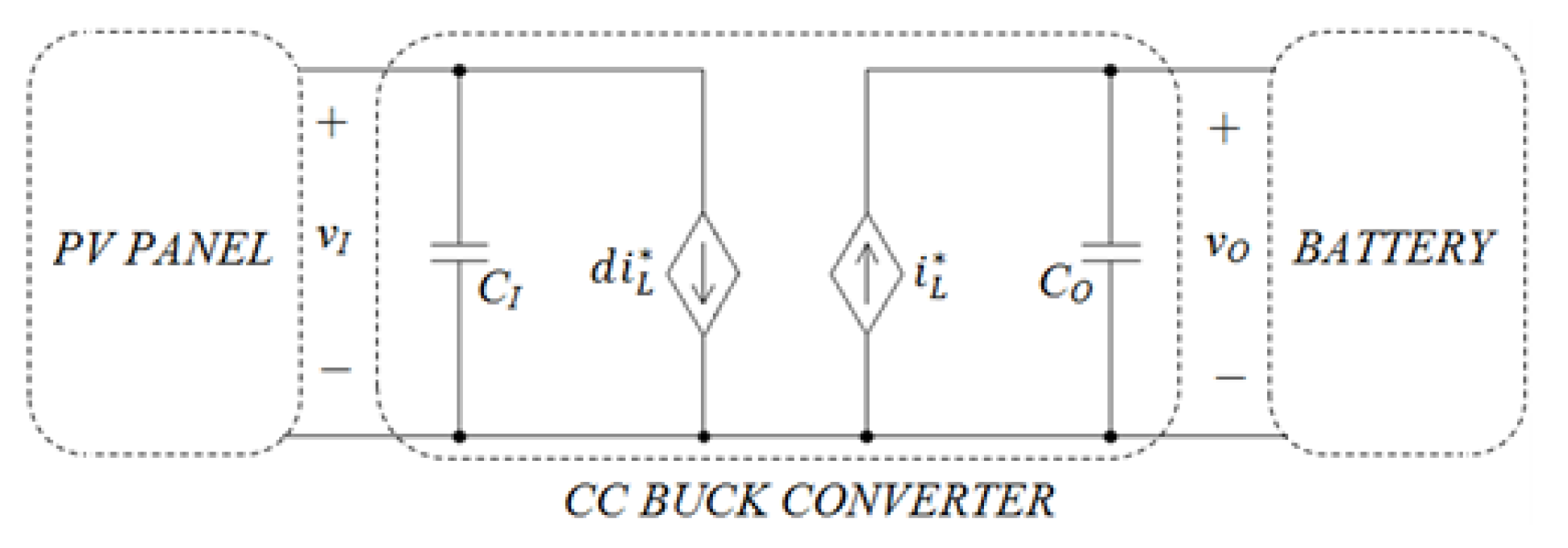
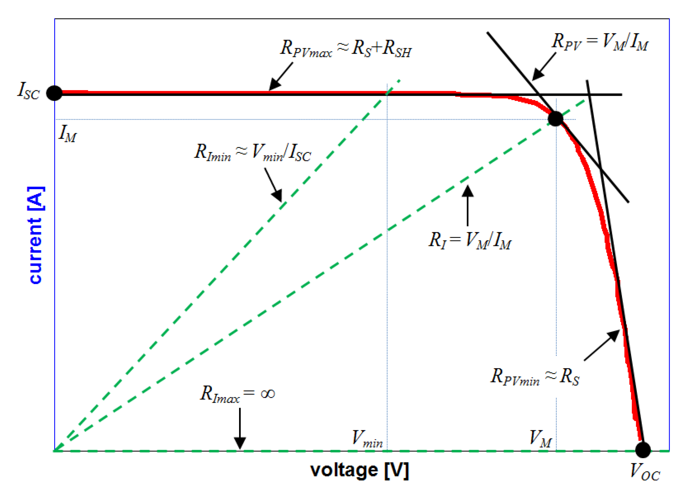
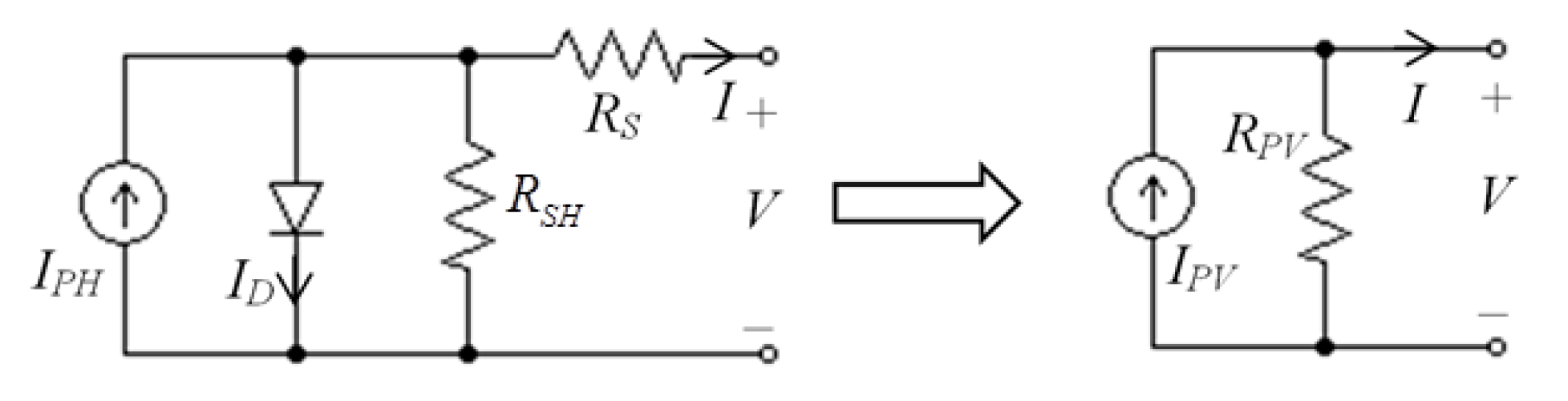
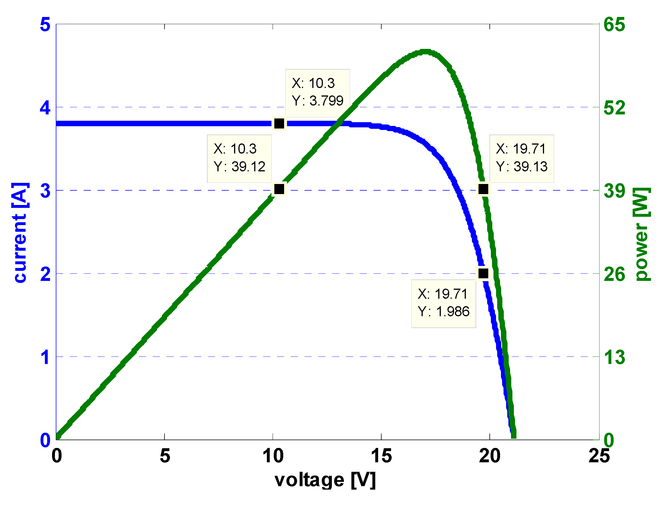
2.2. Solar Array (SA) Modeling for Large and Small Signal Analysis

2.3. System Analysis

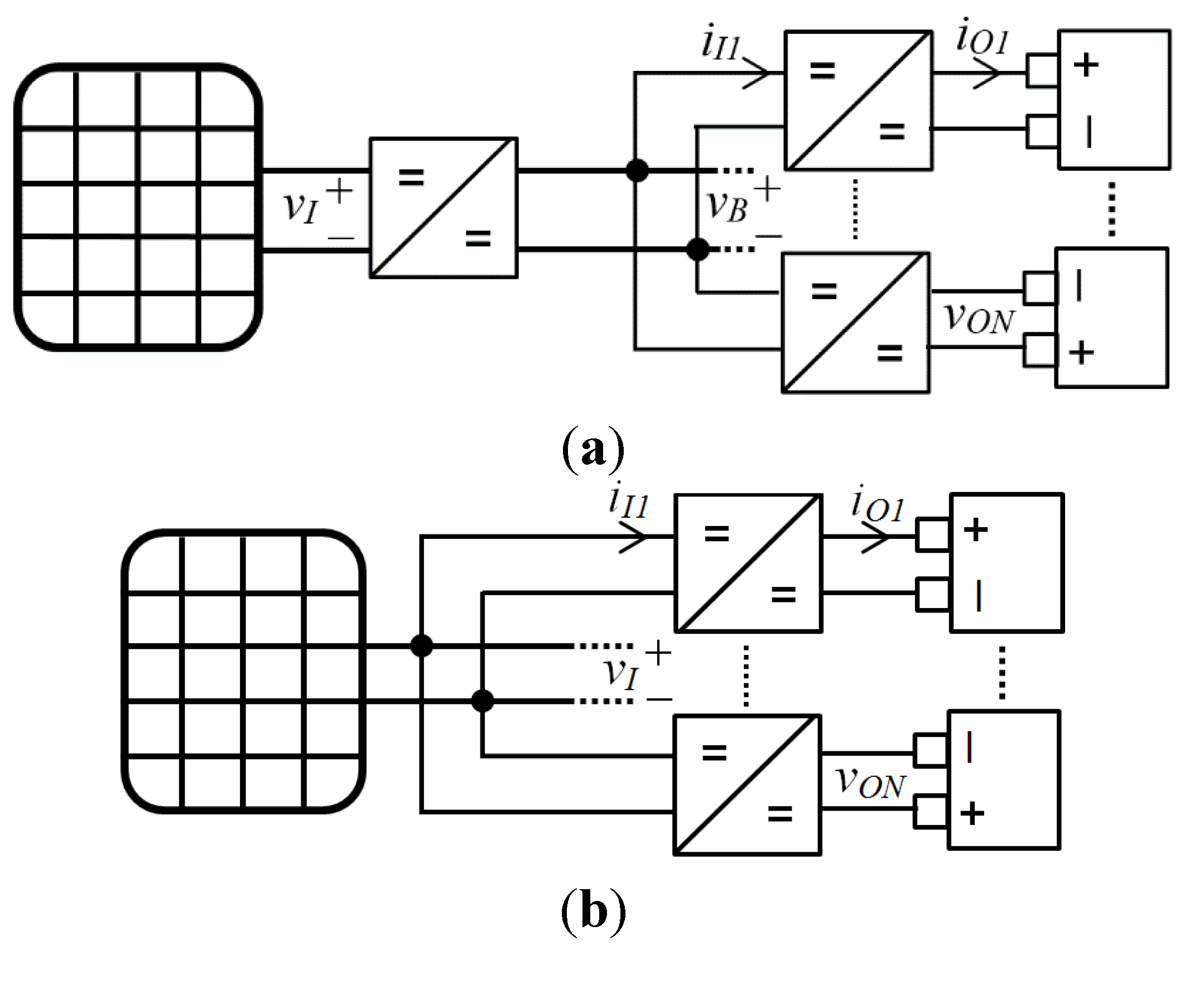
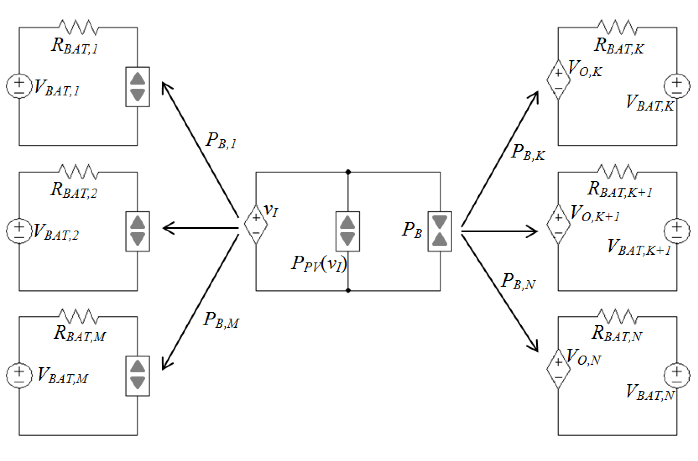
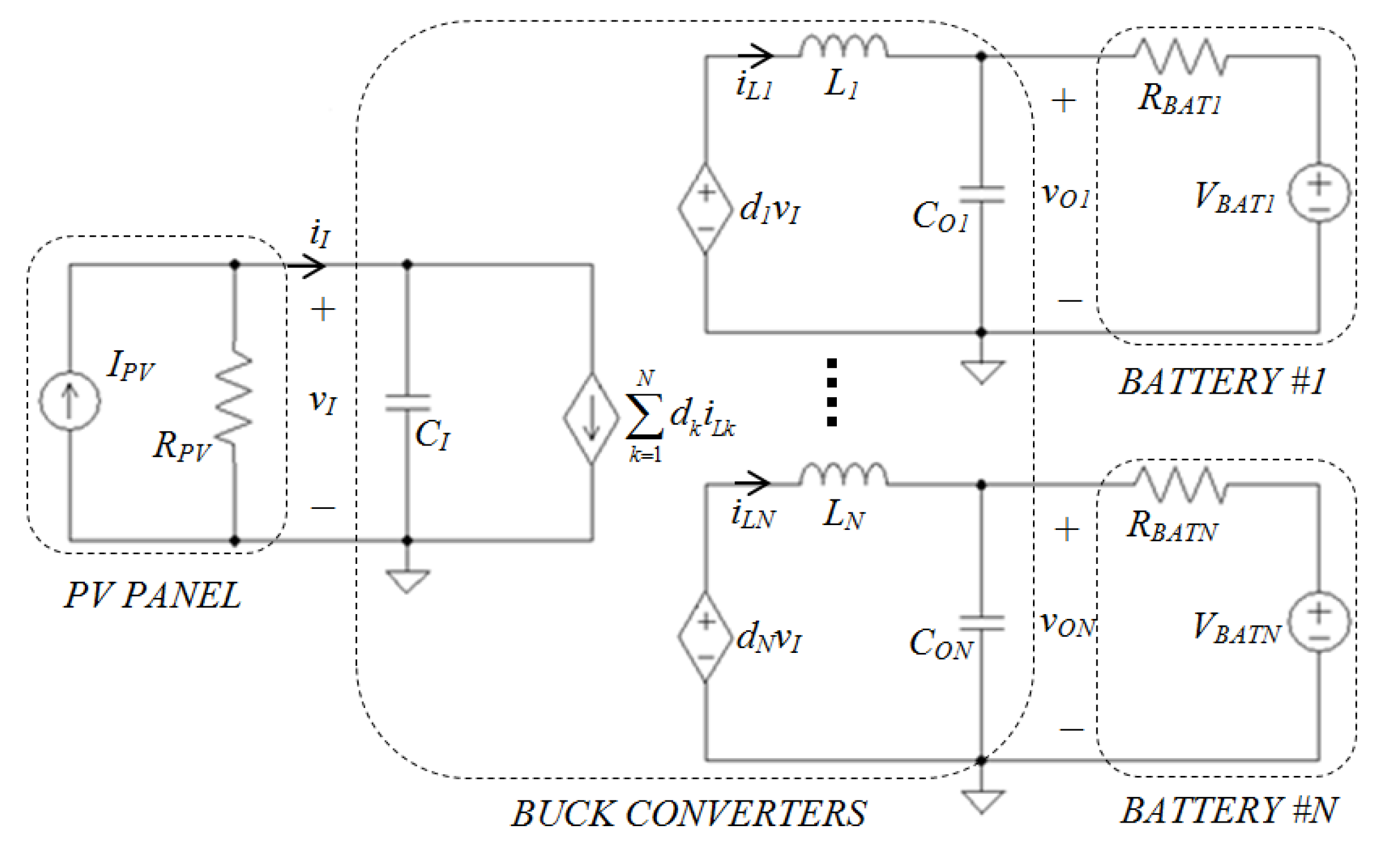
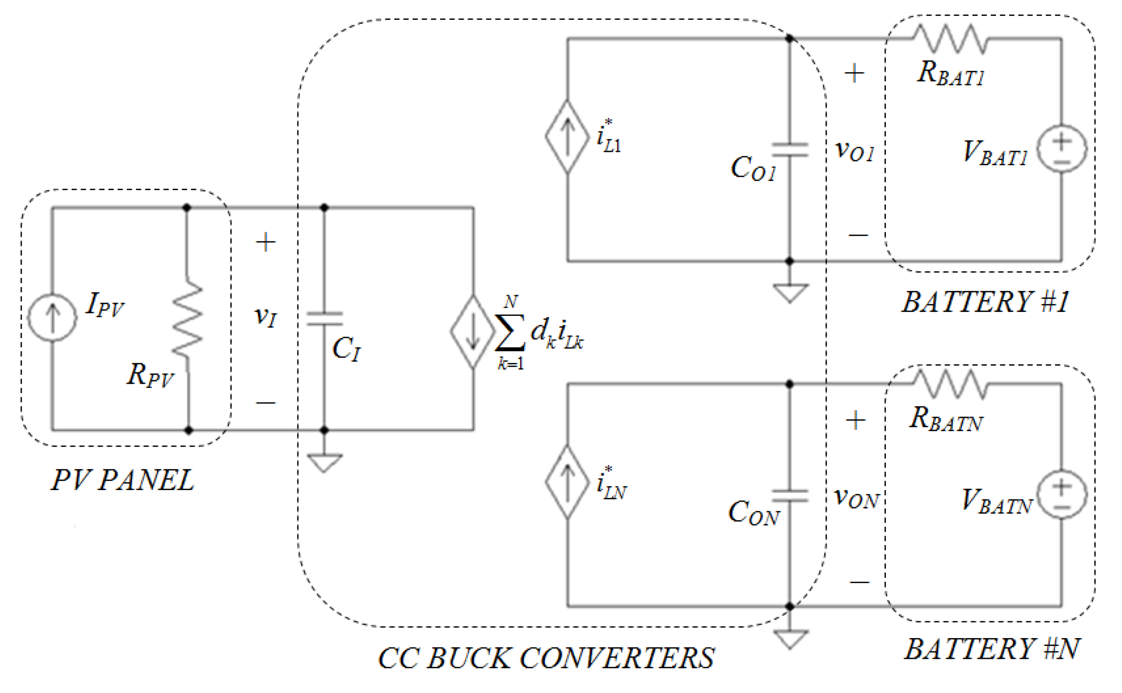
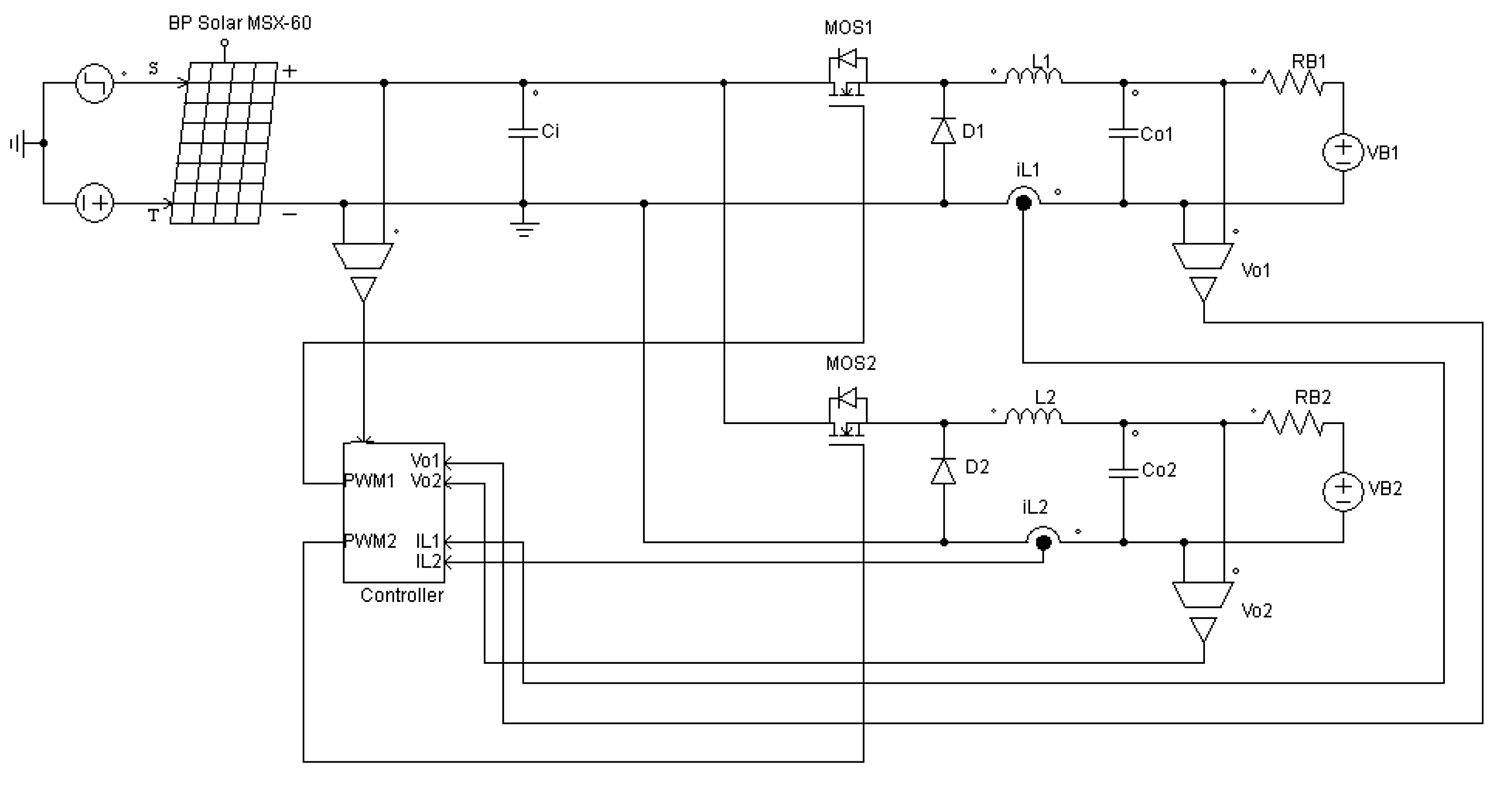
3. Extension to Multi-Battery Case

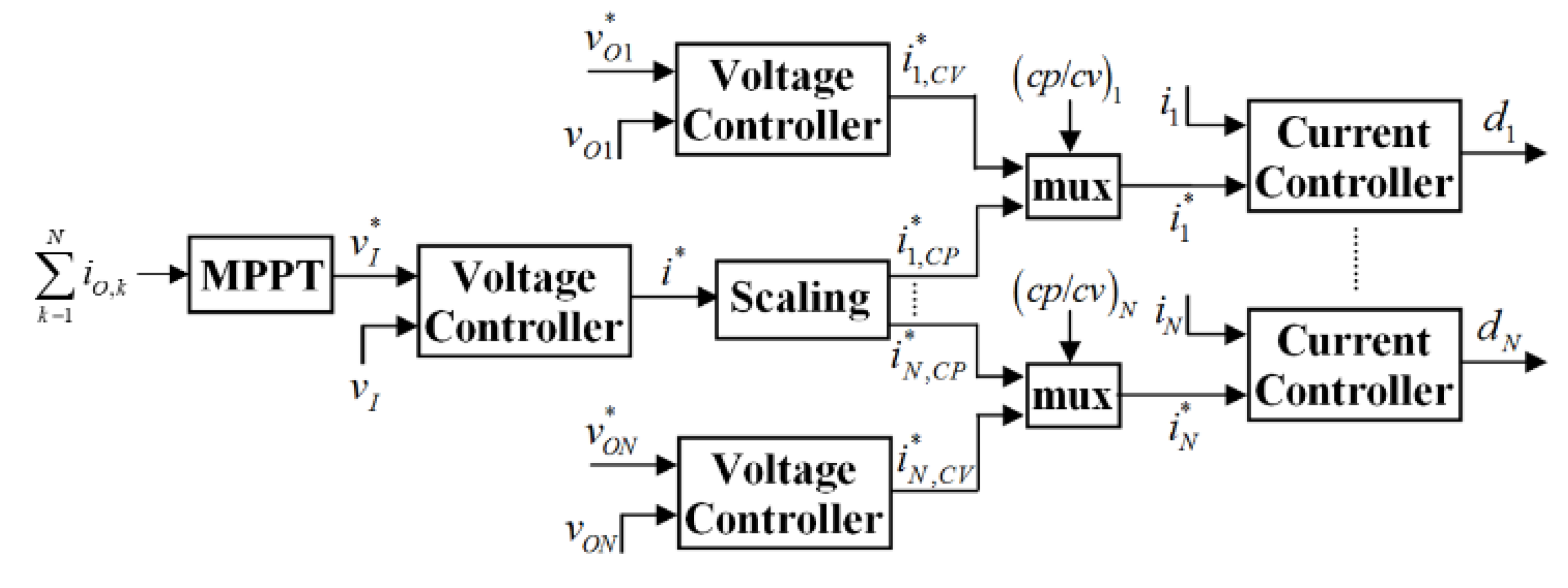


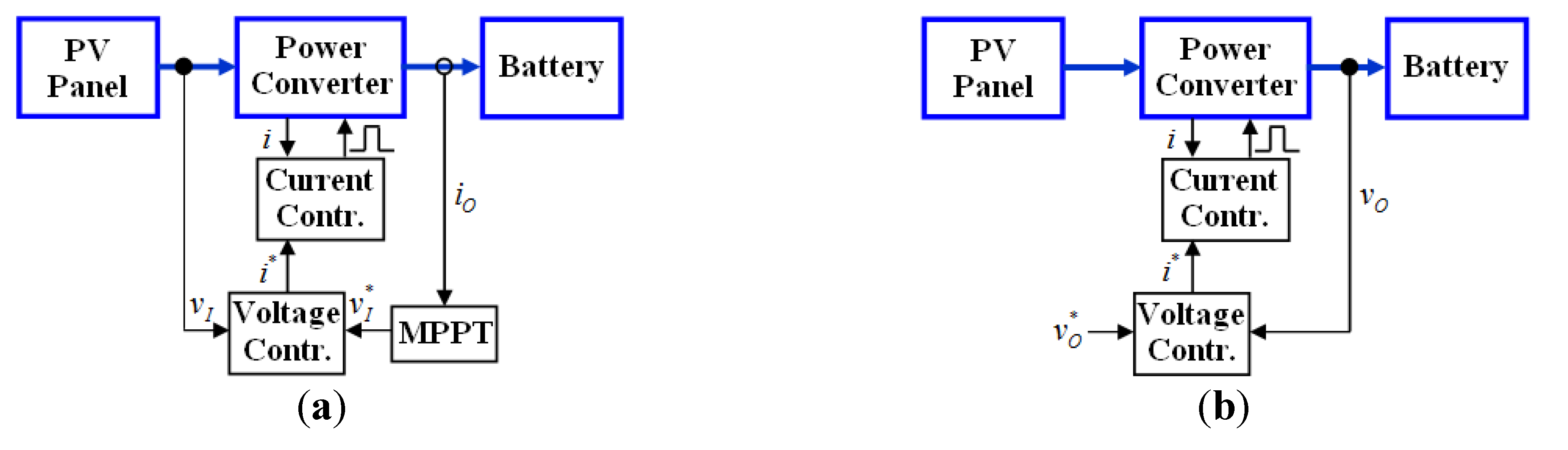
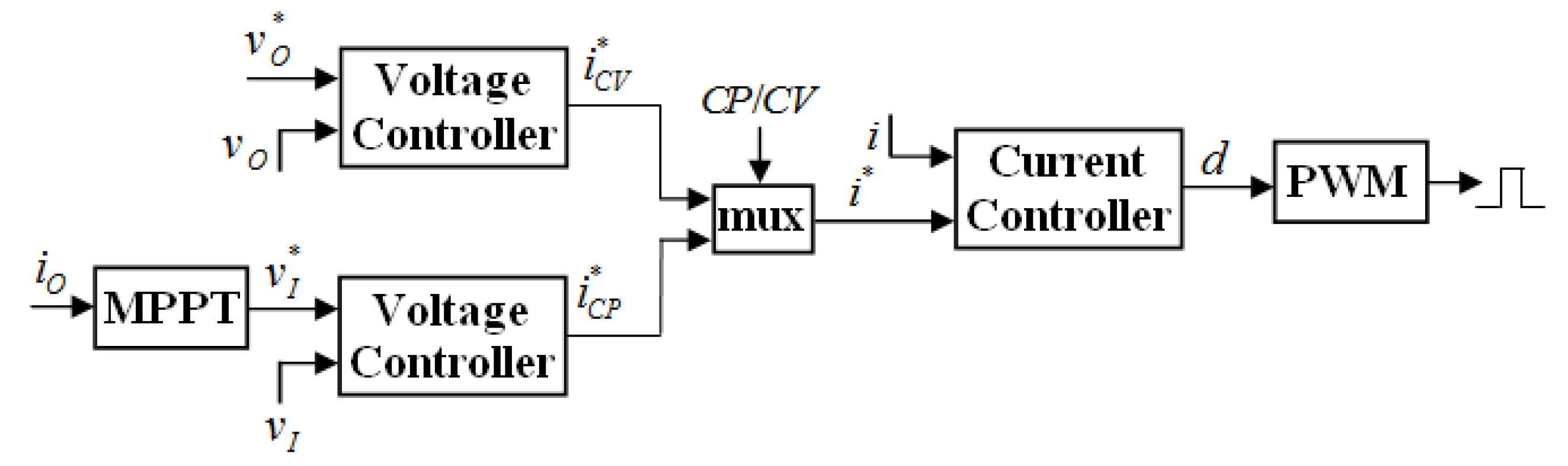
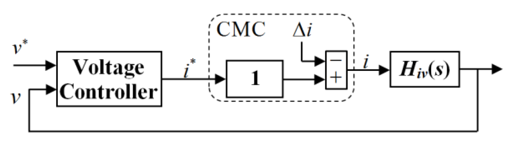
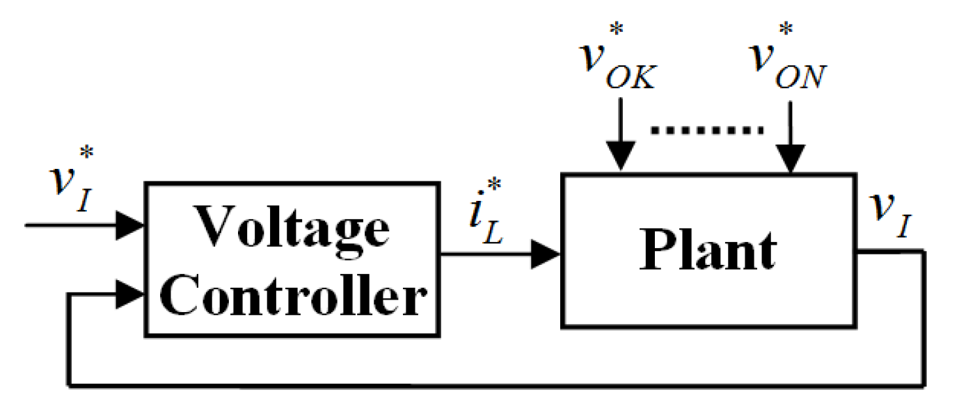
4. Control Design
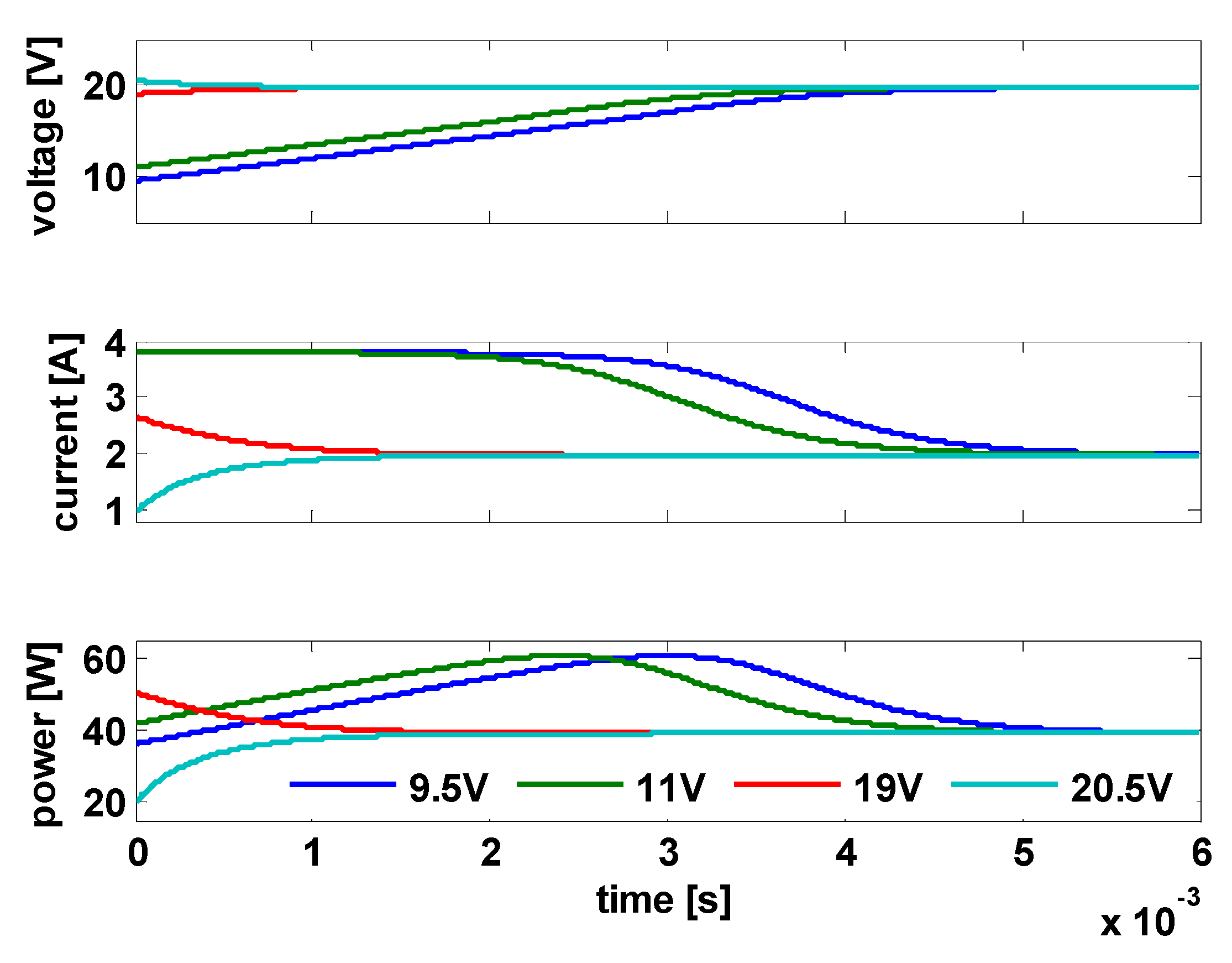
5. Demonstration

| Parameter | Value |
|---|---|
| Open circuit voltage | 21.1 V |
| Short circuit current | 3.8 A |
| Maximum power voltage | 17.1 V |
| Maximum power current | 3.5 A |
| Rated power | 60 W |
| Power temperature coefficient | −0.5%/°C |
| Voltage temperature coefficient | −80 mV/°C |
| Current temperature coefficient | 0.065%/°C |


6. Conclusions
Author Contributions
Conflicts of Interest
Abbreviations
| SA | Solar array |
| PWM | Pulse Width Modulation |
| IC | Integrated Circuit |
| MPP | Maximum Power Point |
| MPPT | Maximum Power Point Tracking |
| LPP | Limited Power Point |
| CP | Constant Power |
| CV | Constant Voltage |
| CMC | Current Mode Control |
| PI | Proportional Integrative |
Nomenclature
battery power | |
solar array power | |
converter input power | |
battery equivalent series resistance | |
battery electro-motive force | |
solar array photocurrent | |
solar array reverse saturation current | |
solar array thermal voltage | |
solar array ideality factor | |
solar array series resistance | |
solar array shunt resistance | |
converter output voltage | |
converter output current | |
converter input voltage | |
converter input current | |
converter inductor current | |
converter input capacitance | |
converter output capacitance | |
converter duty cycle | |
converter efficiency | |
| x* | reference value of variable x |
small-signal value of variable x | |
| X | steady-state value of variable x |
References
- Bragard, M.; Soltau, N.; Thomas, S.; De Doncker, R.W. The balance of renewable sources and user demands in grids: Power electronics for modular battery energy storage systems. IEEE Trans. Power Electron. 2010, 25, 3049–3056. [Google Scholar] [CrossRef]
- Zhou, H.; Bhattacharya, T.; Tran, D.; Siew, T.S.T.; Khambadkone, A.M. Composite energy storage system involving battery and ultracapacitor with dynamic energy management in microgrid applications. IEEE Trans. Power Electron. 2011, 26, 923–930. [Google Scholar] [CrossRef]
- Sun, K.; Zhang, L.; Xing, Y.; Guerrero, J. A distributed control strategy based on DC bus signaling for modular photovoltaic generation systems with battery energy storage. IEEE Trans. Power Electron. 2011, 26, 3032–3045. [Google Scholar] [CrossRef]
- Locment, F.; Sechilariu, M.; Houssamo, I. DC load and battery control limitations for photovoltaic systems. Experimental validation. IEEE Trans. Power Electron. 2012, 27, 4030–4038. [Google Scholar] [CrossRef]
- Dragicevic, T.; Guerrero, J.; Vasquez, J.; Skrlec, D. Supervisory control of an adaptive-droop regulated DC microgrid with battery management capability. IEEE Trans. Power Electron. 2013, 29, 695–706. [Google Scholar] [CrossRef]
- Fakham, H.; Lu, D.; Francois, B. Power control design of a battery charger in a hybrid active PV generator for load-following applications. IEEE Trans. Ind. Electron. 2011, 58, 85–94. [Google Scholar] [CrossRef]
- Indu Rani, B.; Sravana Ilango, G.; Nagami, C. Control strategy for power flow management in a PV system supplying DC loads. IEEE Trans. Ind. Electron. 2013, 60, 3185–3194. [Google Scholar] [CrossRef]
- Aharon, I.; Kuperman, A. Topological overview of battery powered vehicles with range extenders. IEEE Trans. Power Electron. 2011, 26, 868–876. [Google Scholar] [CrossRef]
- Gadelovits, S.; Kuperman, A.; Sitbon, M.; Aharon, I.; Singer, S. Interfacing renewable energy sources for maximum power transfer—Part I: Statics. Renew. Sustain. Energy Rev. 2014, 31, 501–508. [Google Scholar] [CrossRef]
- Urtasun, A.; Sanchis, P.; Marroyo, L. Adaptive voltage control of the DC/DC boost stage in PV converters with small input capacitor. IEEE Trans. Power Electron. 2013, 28, 5038–5048. [Google Scholar] [CrossRef]
- Lu, D.; Agelidis, V. Photovoltaic-battery-powered DC bus system for common portable electronic devices. IEEE Trans. Power Electron. 2009, 24, 849–855. [Google Scholar] [CrossRef]
- Ongaro, F.; Saggini, S.; Mattavelli, P. Li-Ion battery-supercapacitor hybrid storage system for a long lifetime, photovoltaic-based wireless sensor network. IEEE Trans. Power Electron. 2012, 27, 3944–3952. [Google Scholar] [CrossRef]
- Kim, H.; Parkhideh, B.; Bongers, T.; Gao, H. Reconfigurable solar converter: A single-stage power conversion PV-battery system. IEEE Trans. Power Electron. 2013, 28, 3788–3797. [Google Scholar] [CrossRef]
- Barreto, L.; Praca, P.; Oliveira, D.; Silva, R. High-voltage gain boost converter based on three-state commutation cell for battery charging using PV panels in a single conversion stage. IEEE Trans. Power Electron. 2014, 29, 150–158. [Google Scholar] [CrossRef]
- Harrington, S.; Dunlop, J. Battery charge controller characteristics in photovoltaic systems. IEEE Aerosp. Electron. Syst. Mag. 1992, 7, 15–21. [Google Scholar] [CrossRef]
- Boico, F.; Lehman, B.; Shujaee, K. Solar battery charger for NiMH batteries. IEEE Trans. Power Electron. 2007, 22, 1600–1609. [Google Scholar] [CrossRef]
- Carli, G.; Williamson, S. Technical considerations on power conversion for electric and plug-in hybrid electric vehicle battery charging in photovoltaic installations. IEEE Trans. Power Electron. 2013, 28, 5784–5792. [Google Scholar] [CrossRef]
- Siri, K. Study of system instability in solar-array-based power systems. IEEE Trans. Aerosp. Electron. Syst. 2000, 36, 957–964. [Google Scholar] [CrossRef]
- Leppaaho, J.; Suntio, T. Characterizing the dynamics of the peak-current-mode-controlled buck power stage converter in photovoltaic applications. IEEE Trans. Power Electron. 2014, 29, 3840–3847. [Google Scholar] [CrossRef]
- Vesti, S.; Suntio, T.; Oliver, J.; Prieto, R.; Cobos, J. Effect of control method on impedance-based interactions in a buck converter. IEEE Trans. Power Electron. 2013, 28, 5311–5322. [Google Scholar] [CrossRef]
- Anand, S.; Fernandes, B.; Guerrero, M. Distributed control to ensure proportional load-sharing and improve voltage regulation in low-voltage DC microgrids. IEEE Trans. Power Electron. 2013, 28, 1900–1913. [Google Scholar] [CrossRef]
- He, J.; Li, Y.-W. An enhanced microgrid load demand sharing strategy. IEEE Trans. Power Electron. 2012, 27, 3984–3995. [Google Scholar] [CrossRef]
- Urayai, C.; Amaratunga, G.A.J. Single-sensor maximum power point tracking algorithms. IET Renew. Power Gener. 2013, 7, 82–88. [Google Scholar] [CrossRef]
- Shmilovitz, D. On the control of photovoltaic maximum power point tracker via output parameters. IEE Proc. Electr. Power Appl. 2005, 152, 239–248. [Google Scholar] [CrossRef]
- Kuperman, A.; Levy, U.; Goren, J.; Zafransky, A.; Savernin, A. Battery charger for electric vehicle traction battery switch station. IEEE Trans. Ind. Electron. 2013, 12, 5391–5399. [Google Scholar] [CrossRef]
- Lineykin, S.; Averbukh, M.; Kuperman, A. An improved approach to extracting the single-diode equivalent circuit parameters of a photovoltaic cell/panel. Renew. Sustain. Energy Rev. 2014, 30, 282–289. [Google Scholar] [CrossRef]
- Lineykin, S.; Averbukh, M.; Kuperman, A. Issues in modeling amorphous silicon photovoltaic modules by single-diode equivalent circuit. IEEE Trans. Ind. Electron. 2014, 61, 6785–6793. [Google Scholar] [CrossRef]
- Nousiainen, L.; Puukko, J.; Maki, A.; Messo, T.; Huusari, J.; Jokipii, J.; Viinamaki, J.; Lobera, D.T.; Valkealahti, S.; Suntio, T. Photovoltaic generator as an input source for power electronic converters. IEEE Trans. Power Electron. 2013, 28, 3028–3038. [Google Scholar] [CrossRef]
- Pavlovic, T.; Bjazic, T.; Ban, Z. Simplified averaged models of DC-DC power converters suitable for controller design and microgrid simulation. IEEE Trans. Power Electron. 2013, 28, 3266–3275. [Google Scholar] [CrossRef]
- Kuperman, A. Comments on “An analytical solution for tracking photovoltaic module MPP”. IEEE J. Photovolt. 2014, 4, 734–735. [Google Scholar] [CrossRef]
- Messo, T.; Jokipii, J.; Puukko, J.; Suntio, T. Determining the value of DC-link capacitance to ensure stable operation of a three-phase photovoltaic inverter. IEEE Trans. Power Electron. 2014, 29, 665–673. [Google Scholar] [CrossRef]
- Gadelovits, S.; Sitbon, M.; Suntio, T.; Kuperman, A. Single-source multi-battery solar charger: Case study and implementation issues. Prog. Photovolt. Res. Appl. 2015. [Google Scholar] [CrossRef]
© 2015 by the authors; licensee MDPI, Basel, Switzerland. This article is an open access article distributed under the terms and conditions of the Creative Commons Attribution license (http://creativecommons.org/licenses/by/4.0/).
Share and Cite
Kuperman, A.; Sitbon, M.; Gadelovits, S.; Averbukh, M.; Suntio, T. Single-Source Multi-Battery Solar Charger: Analysis and Stability Issues. Energies 2015, 8, 6427-6450. https://doi.org/10.3390/en8076427
Kuperman A, Sitbon M, Gadelovits S, Averbukh M, Suntio T. Single-Source Multi-Battery Solar Charger: Analysis and Stability Issues. Energies. 2015; 8(7):6427-6450. https://doi.org/10.3390/en8076427
Chicago/Turabian StyleKuperman, Alon, Moshe Sitbon, Shlomo Gadelovits, Moshe Averbukh, and Teuvo Suntio. 2015. "Single-Source Multi-Battery Solar Charger: Analysis and Stability Issues" Energies 8, no. 7: 6427-6450. https://doi.org/10.3390/en8076427