Optimization and Analysis of a Hybrid Energy Storage System in a Small-Scale Standalone Microgrid for Remote Area Power Supply (RAPS)

Abstract

The analysis and application of hybrid energy storage systems (HESSs) in small-scale standalone microgrids for remote area power supply (RAPS) has received extensive attention. This application mode has its own characteristics which must be considered but have not been considered in the existing research. To reflect the common satisfaction of load demands and maximize the utilization of renewable energy in a standalone microgrid, a new index named effective rate of energy storage system (ESS) is proposed. To reflect the true work state of supercapacitor ESS (SC-ESS), the second-level data of field measurements is used in calculation and analysis. To further enhance the operational performance of the HESS, a coordinated control strategy based on state cooperation is adopted. To get a more reasonable and more credible HESS optimization model, the comparison of existing models and proposed model with different considerations on cost and life is provided. In addition, a comparative analysis of technical and economic characteristics improvements is presented for different ESS application schemes in practical projects.

1. Introduction

The utilization of renewable energy sources, such as wind-turbine power generation (WT), photovoltaic power generation (PV), etc., can effectively alleviate the increasingly serious problems of energy crisis and environmental pollution. However, there are still some remote areas not suitable for independently getting their power supply from large power grids or small conventional power generators due to economic, environmental and other factors. However, these areas are often rich in wind energy and solar energy which can be used as distributed generation and to constitute a small standalone RAPS system [1,2]. These small systems, called standalone microgrids, are an effective way of solving the problem of villages in remote areas without electricity. WT and PV can exist simultaneously or only partially in a standalone microgrid. Wind energy and solar energy themselves are both random and uncontrollable, so their output power can’t satisfy the time-varying load demands. ESSs can not only provide voltage and frequency support in the form of a main power supply to maintain system stability, but also have many advantages such as environmental-friendliness, bidirectional flow of energy, and continuously adjustable charge-discharge power features. Therefore, ESSs have become an important part of such standalone microgrids [3,4,5].

Energy storage technology can be divided into energy type and power type. The former has a large storage capacity and short life cycle, while the latter has a large power density, fast response and long life cycle. In recent years, energy-type energy storage devices have been commonly used in standalone microgrids including renewable energy generation [6,7,8,9,10], but the face the challenge of large fluctuation in charge-discharge power, and even the challenge of frequent switching between charge-discharge status. This will accelerate the life loss of energy-type energy storage systems which are sensitive to the charge-discharge process, and severely degrade their performance. If the two types of energy storage are used as a whole, namely HESS, complementarity of technical characteristics can be achieved. The typical HESS, which consists of lithium-ion battery ESS (LB-ESS) and SC-ESS, is commonly used in RASP systems [11,12,13,14,15,16,17].

The parameters such as power rating and storage capacity of each sub-ESS, which can directly affect the overall technical and economic characteristics of HESS, should be optimized. In [18], the supercapacitor was increased to meet the peak load and reduce the battery capacity configuration in a PV independent power supply system. In a stand-alone power system with single source HESS described in [19], the power rating and storage capacity configurations for two ESSs have been analyzed, and the comparison between a HESS and a single energy storage system (SESS) is given. A method for configuring HESS capacities for a WT/PV autonomous multi-microgrids cluster has been presented [20] based on the maximum off-grid time of allowable continuous running, and the expected stable system operation time under extreme conditions. Capacity optimization of battery arrays and supercapacitor arrays are proposed to minimize one-time investment and operation costs for a WT/PV standalone system in [21]. The optimization results of HESS based on the total cost is given in [22] for a PV off-grid power system. The sum of capital cost and balancing cost is the objective function of the total cost optimization in a WT independent system described in [23], and the results show that HESS is better than SESS.

Through analysis, research on HESS optimization of independent microgrids should be focused on HESS control strategy, data interval, cost consideration factors, energy storage life quantization and system constraints. In addition to [19] using a first-order filter to allocate load power, HESSs in the above studies are all controlled by a simple rule, i.e., batteries to meet the load energy demand and supercapacitors to meet the instantaneous pulse loads. The technological complementarities of HESS can’t be fully utilized because there is no coordination between the two types of ESSs. In a small-scale RAPS stand-alone microgrid, the storage capacity of SC-ESS can’t be too large based on the considerations of application requirements and economic cost. In general, the rated power discharge duration of a SC-ESS is no more than several hundred seconds. However, the data interval of WT, PV and load in these studies can be basically one hour, or even a month [21], and the true working states of SC-ESS are not reflected. The storage arrays are connected to the power supply system through a Power Convert System (PCS), so a HESS consists of several sub-ESSs storage array components and the corresponding PCSs. The optimization considering cost of storage arrays alone will affect the credibility of the study results.  At the same time, the battery life quantification is considered only in [19], and battery life is simply computed as an equivalent number of charge-discharge cycles. There is no consideration of life quantization for supercapacitors and PCSs. Further, Loss of Power Supply Probability (LPSP) or Loss of Load Probability (LOLP) [20,22,23] are taken as system constraints in the above HESS optimizations of independent microgrids. The indexes only reflect the satisfaction of load power, and can’t accurately reflect the system requirements when renewable generation is included.

Aiming at the insufficiencies of existing research, a new index is proposed in this paper to accurately reflect the satisfactory rate of net load in a standalone microgrid. In order to reflect the true work state of SC-ESS, field measurements data with small enough time intervals is used for calculation and analysis. Compared with considering only power allocation in HESS control, the necessity of using the coordinated control strategy based on state cooperation is analyzed. Optimization models are established to reflect the impact of HESS optimization without a comprehensive consideration of cost and life, and to analyze the merits of common ESS application schemes in practical projects.

2. A Small-Scale Standalone Microgrid and ESSs

2.1. System Structure of a Standalone Microgrid for RAPS

A RAPS system described above is a small-scale off-grid system consisting of loads, ESSs and distributed renewable energy generation. The system is a standalone microgrid taking ESSs as the main power supply for power balance and system stability. A system structure of the microgrid for AC applications considered in this paper is shown in Figure 1.

The load demands are the requirement of time-varying power from AC BUS to the load shown as P_LD in Figure 1. P_DG shown in Figure 1 is the sum of output powers of distributed generation sent to the AC BUS. The distributed generation consists of renewable energy generation sources, such as WT, PV and so on, which should be utilized as much as possible. The distributed generation sources can’t maintain the system stability and power balance because their output powers are random, intermittent and uncontrollable. The balance node is ESSs which can absorb and output power satisfying the system requirement within the allowable range. HESS or SESS consisting of energy-type ESS can be used here. P_{out_ESS} shown in Figure 1 is the total charge-discharge power of ESSs, i.e., the bi-directional power flow between ESSs and the AC BUS. At the same time, the sum of load demands and distributed generations can be regarded as the net load of this system P_{net_LD} shown in Figure 1. If the direction to AC BUS is defined as the positive direction, the values of P_LD and P_DG are negative and positive, respectively, and the values of P_{out_ESS} and P_{net_LD} both can be positive or negative.

Figure 1. Configuration diagram of a standalone microgrid.

Figure 1. Configuration diagram of a standalone microgrid.

2.2. The Proposed Index Named ESS Effective Rate

In the existing research on HESS optimization in standalone microgrids, the indexes LPSP or LOLP are used as system constraints [20,22,23]. As some of the most common reliability indices, LPSP and LOLP are both indexes that show the system performance under a particular load. LPSP or LOLP actually are the ratio of load energy shortage and total load energy demand as shown as Equation (1), which ranges from 0 to 100%. In the discrete calculation with the same time interval, this value is equal to the ratio of load power shortage and total load power demand. When LPSP or LOLP is equal to 100%, the load is never satisfied and the system should be redesigned. When LPSP or LOLP is equal to 0, the system is able to supply the power to the load all the time:

$$L_{pro}=100\%\times {\displaystyle \sum _{n=1}^{N_T}\left\{P_{loss\_LD(n)}\cdot \text{Δ}{T}_{com}\right\}}/{\displaystyle \sum _{n=1}^{N_T}\left\{P_{LD(n)}\cdot \text{Δ}{T}_{com}\right\}}$$

(1)

According to the positive direction as shown in Section 2.1, the value of load is negative because it absorbs energy from the AC bus, and the value of DG output is positive because it outputs energy to the AC bus. Therefore, the value of load energy shortage and total load energy demand are both negative. When P_LD + P_DG ≤ 0, the DG output is equal to or less than the load demand. In this case, the microgrid is under the state of power requirement, and this can be cumulatively calculated in LPSP or LOLP. When P_LD + P_DG > 0, the DG output is more than the load demand, and the power supply of microgrid is in an overabundance with respect to the load demand. Although this state often occurs in actual operation, it can’t be reflected in the calculation of LPSP or LOLP. In other words, the indexes LPSP or LOLP can only count the negative part of the net load which is the sum of load demand and DG output, as shown in Equation (2):

$$P_{loss\_LD(n)}=\min \left\{P_{LD(n)}+P_{DG(n)},0\right\}=-\left|P_{net\_LD(n)}\right|$$

(2)

However, in the standalone microgrid which is different from the traditional power grid, not only should the load demand be met, but also renewable energy generation sources should be utilized as much as possible. When all the renewable energy generation output power has been fully utilized, a new index is needed to show the system performance under the particular load and renewable energy generation situation. Therefore, the effective rate of ESS is proposed to reflect the degree to which the net load demand is satisfied. The effective rate R_ESS is computed using Equation (3). In order to get the power balance of a microgrid system, the sum of DG output, load power demand and ESS output should be equal to 0, so the reference value of ESS power output is calculated using Equation (4):

$$R_{ESS}=\begin{array}{c}(1-\frac{{\displaystyle \sum _{n=1}^{N_T}\left\{\left|P_{ref\_ESS(n)}-P_{out\_ESS(n)}\right|\cdot \text{Δ}{T}_{com}\right\}}}{{\displaystyle \sum _{n=1}^{N_T}\left\{\left|P_{ref\_ESS(n)}\right|\cdot \text{Δ}{T}_{com}\right\}}}\end{array})\times 100\%$$

(3)

$$P_{ref\_ESS(n)}=-(P_{LD(n)}+P_{DG(n)})=-P_{net\_LD(n)}$$

(4)

The subscript “_ESS” represents the current ESS, which can be SESS or HESS. The numerical range of R_ESS is [0, 100%]. In a standalone microgrid taking ESS as balance node, the smaller the difference between the actual output power of the ESS and the net load is, the bigger the value of R_ESS is, and the higher the requirements for ESS. Only when the two above are always exactly equal, R_ESS is 100%. Similar with the reliability requirement, the constraint of ESS effective rate R_set can be set for optimization analysis of ESS in a standalone microgrid. A penalty cost C_{pen_ESS} is needed because the requirement of effective rate must be satisfied in the optimization. In Equation (5), F is a fixed value which is much bigger than other costs:

$${\text{C}}_{pen\_ESS}=\{\begin{array}{l}0,\\ F,\end{array}\begin{array}{c}\\ \end{array}\begin{array}{c}{R}_{ESS}\ge R_{set}\\ R_{ESS}<R_{set}\end{array}$$

(5)

2.3. General Mathematical Model of ESSs

In order to perform an optimization study of HESS, suitable mathematical models must be established. Although LB and SC have different technical characteristics, they are both energy storage technologies which can be charged and discharged as required through corresponding PCS. A general mathematical model available for LB-ESS and SC-ESS is presented in [24,25,26,27,28,29,30]. As shown in Equations (6)–(8), this model includes the computation of power output limits and state of charge (SOC) for ESSs. Moreover, the effect of self-discharge rate and charge-discharge efficiency is considered making the model more credible and effective:

$$P_{clmt\_ESS\text{(n)}}\text{=}-\text{min{[}{S}_{\max \_ESS}-\text{(1}-{\sigma }_{ESS}\text{)}{S}_{ESS\text{(n-1)}}]\frac{E_{r\_ESS}}{{\eta }_{\text{c}\_ESS}\text{Δ}{T}_{com}}\text{,}\begin{array}{c}\end{array}\left|P_{c\max \_ESS}\right|\text{}}$$

(6)

$$P_{dlmt\_ESS\text{(n)}}\text{=min{[(1}-{\sigma }_{ESS}\text{)}{S}_{ESS\text{(n-1)}}-S_{\min \_ESS}]\frac{{\eta }_{d\_ESS}{E}_{r\_ESS}}{\text{Δ}{T}_{com}}\text{,}\begin{array}{c}\end{array}{P}_{d\max \_ESS}\text{}}$$

(7)

$$S_{ESS\text{(n)}}=\{\begin{array}{c}(1-{\sigma }_{ESS})S_{ESS(n-1)}-P_{out\_ESS}{\eta }_{c\_ESS}\text{Δ}{T}_{com}/E_{r\_ESS},\\ (1-{\sigma }_{ESS})S_{ESS(n-1)}-\frac{P_{out\_ESS}\text{Δ}{T}_{com}}{{\eta }_{d\_ESS}{E}_{r\_ESS}},\begin{array}{cc}& \end{array}\end{array}\begin{array}{c}\\ \end{array}\begin{array}{c}(P_{out\_ESS}\le 0)\\ \\ (P_{out\_ESS}>0)\end{array}$$

(8)

3. Control Strategy of HESS

3.1. The Basic Control Strategy Considering Power Allocation Only

The existing work of HESS control in the standalone microgrid merely focuses on power allocation, and the methods used in [18,19,20,21,22,23] are simple rule and first-order filter. In the simple rule method, SC-ESS is used to meet pulse loads. However, the charge-discharge power of LB-ESS may still be changing rapidly, which will adversely affect the LB life. Although there are some other methods applicable to power allocation in all the research on HESS control, the first-order filtering method is the most common and widely accepted one. Through this method, the high-frequency parts of power fluctuations are borne by SC-ESS, and LB-ESS satisfies the rest, which is relatively flat. This can make full use of the advantages of SC and be conducive to delayed LB life loss. The basic control strategy considering power allocation only is the first-order filtering method shown as Equations (9) and (10):

$$P_{out\_SC}(s)=P_{HESS}(s)\cdot \text{[}s{T}_f/(1+s{T}_f)]$$

(9)

$$P_{out\_LB}(s)=P_{HESS}(s)-P_{out\_SC}(s)=P_{HESS}(s)/(1+s{T}_f)$$

(10)

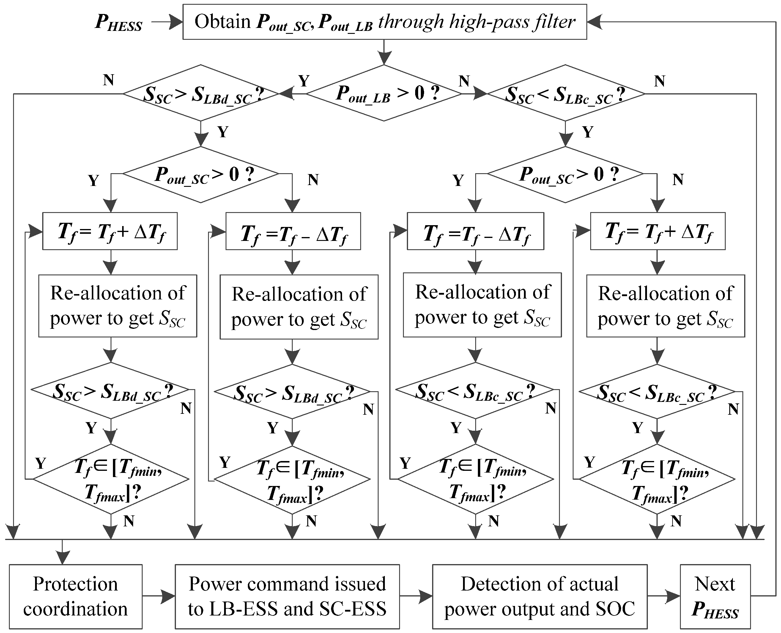
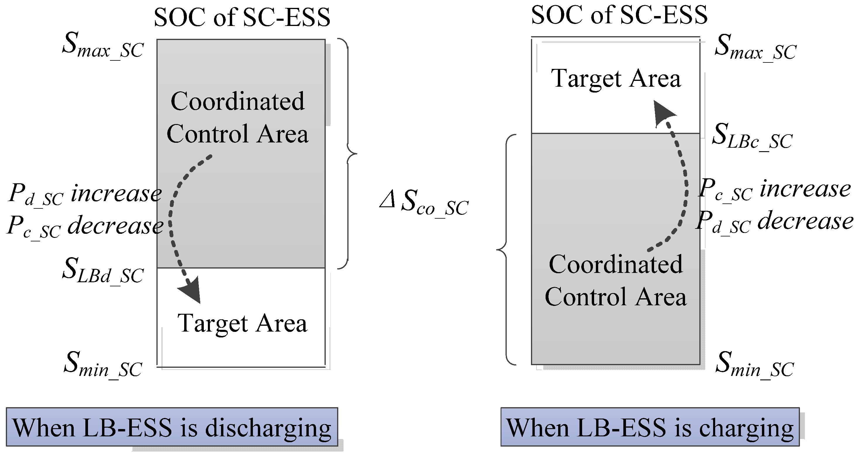
3.2. The Coordinated Control Strategy Based on State Cooperation

In order to optimize the overall adjustment ability and improve the overall performance, the coordination between two HESS ESSs should be considered. A control strategy proposed in [31] considers the state coordination between two ESSs and can improve the overall performance of HESS. The strategy mainly includes four parts: the primary allocation of power commands, status adjustment of SC-ESS, coordination of overcharge and over-discharge protection and coordination of maximum power limit protection. The control flow of this coordinated control strategy based on state cooperation is shown in Figure 2.

The computation of primary allocation is same as Equations (9) and (10), where T_f is the initial value T_f0. When optimizing the overall adjustment ability, T_f can be repeatedly adjusted within the permissible range [T_fmin, T_fmax] in steps of ΔT_f. Figure 3 illustrates the principle of overall adjustment ability optimization as the core part of the coordinated control strategy, where SOC of SC-ESS is dynamically adjusted according to charge-discharge status of LB-ESS [32]. It shows that charging margin is reserved in SC-ESS when LB-ESS is discharging, and discharging margin is reserved in SC-ESS when LB-ESS is charging. Then there will be an enhanced response capability for instantaneous power changes, an optimization of charge and discharge process for SC-ESS, and an improvement of overall performance for HESS. Hence, a new index named as SOC coordinated response margin of SC-ESS is denoted by ΔS_{co_SC}, which is numerically equal to (S_{max_SC} -S_{LBd_SC}) or (S_{LBc_SC} -S_{min_SC}).

Figure 2. Flow chart of the coordinated control strategy for HESS.

Figure 2. Flow chart of the coordinated control strategy for HESS.

Figure 3. Coordination control diagram of overall adjustment.

Figure 3. Coordination control diagram of overall adjustment.

4. Cost Calculation and Life Quantification of HESS

The costs of HESS primarily include the initial investment cost and the loss equivalent cost. The initial investment cost is the purchase and other expenses of HESS, which is a one-time investment cost. The loss equivalent cost is the depreciation expense of HESS within a certain time, which is a comprehensive cost, namely a form of life cycle cost. Owing to the different characteristics of different components, depreciation of HESS can’t simply to use the service life, and the life of different components should be quantified separately.

4.1. Initial Investment Cost of HESS

The HESS in this paper consists of the LB arrays, the SC arrays and the two corresponding PCSs. The energy storage arrays typically consist of energy storage modules with series-parallel connection, which largely determines the ESS storage capacity. The total initial investment cost of LB storage arrays and SC storage arrays is computed by Equation (11). In practical applications, PCS usually is a standard equipment package which largely determines the power limits of ESS. The initial investment cost of PCSs is a fixed value under the determined level of rated power of ESSs. The initial investment cost of LB-ESS, SC-ESS and the whole HESS are computed using Equations (12), (13) and (14):

$$C_{initial\_HESSarr}=C_{unit\_LB}{E}_{r\_LB}+C_{unit\_SC}{E}_{r\_SC}$$

(11)

$$C_{initial\_LB}=C_{unit\_LB}{E}_{r\_LB}+C_{PCS\_LB}$$

(12)

$$C_{initial\_SC}=C_{unit\_SC}{E}_{r\_SC}+C_{PCS\_SC}$$

(13)

$$C_{initial\_HESS}=C_{initial\_LB}+C_{initial\_SC}$$

(14)

4.2. Life Quantification and Loss Equivalent Cost of Storage Arrays in LB-ESS

The useful life of the LB has an important impact on the overall performance of HESS, because the service lifetime of LBs is much shorter than that of other HESS components. Therefore, the quantification life and loss equivalent cost of LB are important indexes measuring the technical and economic characteristics of HESS. The LB lifetime is typically defined as cycle life or calendar life corresponding with the degenerative process from the nominal energy capacity to its 80% level [33,34,35,36]. A LB capacity degradation algorithm suitable for practical applications and irregular charge-discharge applications in particular is proposed in [33], as a function of the equivalent throughput cycles, the average SOC, the normalized SOC deviation and the operating temperature. The algorithm shown in Equation (15) validated by experiments and actual operation has repeatedly been cited or applied directly in [34,35,36,37,38,39,40]:

$$\begin{array}{l}{L}_{array\_LB}={\displaystyle \sum _{m=1}^M\text{Δ}{D}_{LB}}(m)/D_{lmt\_LB}\\ \begin{array}{cc}& \\ & \end{array}\{\begin{array}{l}\text{Δ}{D}_{LB}(m)=D_2\cdot \exp [K_T(T_{LB}-T_{ref})\cdot \frac{T_{a\_ref}}{T_{a\_LI}}]\\ D_2=D_1\cdot \exp [4K_{SOC}(S_{avg\_LB}-0.5)]\cdot [1-D_{LB}(m-1)]\\ D_1=K_{co}{N}_{LB}\cdot \exp (\frac{S_{dev\_LB}-1}{K_{ex}}\cdot \frac{T_{a\_ref}}{T_{a\_LB}})+\frac{0.2\tau }{{\tau }_{life\_LB}}\end{array}\end{array}$$

(15)

where D_{lmt_LB} = 0.2, T_ref =25 °C, T_{a_ref} = T_ref +273, T_{a_LB} = T_LB + 273, K_T = 0.0693, K_co = 3.66e-5, K_ex = 0.717, K_SOC = 0.916 [33]. The coefficients K_T, K_co, K_ex, K_SOC are typical values used as empirical constants of a particular LB, and can be amended in accordance with the lifetime data for different LBs. The degradation of LB capacity changes from 0 (when LB is new) to 1 (when the capacity of LB degenerates to 0). D_{lmt_LB} = 0.2 means that the actual capacity of LB degenerates to 80% of its nominal capacity. The cycle uses number or usage time length from 0 to D_{lmt_LB}, namely cycle life or calendar life of LB.

The loss equivalent cost considering life quantification of storage arrays in LB-ESS is computed as follows:

$$C_{loss\_LBarr}=L_{array\_LB}{C}_{array\_LB}$$

(16)

4.3. Overall Life Quantification and Total Loss Equivalent Cost of HESS

In order to more accurately reflect the performance of HESS, the life of each component should be quantified. The number of SC charge-discharge cycles is more than one million times, which is more than LB as shown in [15,41], soan approximate calculation model is used for lifetime quantization of SC arrays. The lifetime loss coefficient of storage arrays in SC-ESS is approximately the ratio of used cycles and its total cycles, which is computed by Equation (17). The loss equivalent cost considering life quantification of storage arrays in SC-ESS is computed with Equation (18):

$$L_{array\_SC}=N_{cycle\_SC}/N_{total\_SC}$$

(17)

$$C_{loss\_SCarr}=L_{array\_SC}{C}_{array\_SC}$$

(18)

Various PCSs used in LB-ESS and SC-ESS usually work uninterruptedly, and their power electronic devices have a limited service lifetime. Without taking into account any failure, the lifetime loss coefficient of PCS is approximately the ratio of running time and corresponding service lifetime. The coefficient is computed by Equation (19):

$$L_{loss\_PCS}=T/T_{life\_PCS}$$

(19)

The total loss equivalent cost of each ESS and HESS are computed as follows:

$$C_{loss\_LB}=C_{loss\_LBarr}+L_{loss\_PCS}{C}_{PCS\_LB}$$

(20)

$$C_{loss\_SC}=C_{loss\_SCarr}+L_{loss\_PCS}{C}_{PCS\_SC}$$

(21)

$$C_{loss\_HESS}=C_{loss\_LB}+C_{loss\_SC}$$

(22)

4.4. Impact Analysis Models of Different Cost and Life Considerations

The consideration of cost and life in optimization of HESS is not comprehensive in the existing research [18,19,20,21,22,23], and the optimized results may not be the best overall. In this paper, an overall optimization model shown by Equation (26) is established considering the life quantification and cost conversion of each HESS component. For comparative analysis, three different optimization objective functions based on different cost and life considerations, shown as Equations (23), (24) and (25), are set to indicate the lack of existing research. The total initial investment cost and total loss equivalent cost of HESS in four different optimized results are compared to analyze the changes of overall technical and economic characteristics of HESS. The HESSs all use the coordinated control strategy based on state cooperation, and satisfy the net load demand of a standalone microgrid for RAPS.

Optimization Objective 1, to minimize the total initial investment cost of storage arrays in HESS:

$$\min (C_{opt1\_HESS})=\min (C_{initial\_HESSarr}+C_{pen\_ESS})$$

(23)

Optimization Objective 2, to minimize the initial investment cost of the whole HESS:

$$\min (C_{opt2\_HESS})=\min (C_{initial\_HESS}+C_{pen\_ESS})$$

(24)

Optimization Objective 3, to minimize the loss equivalent cost of storage arrays of LB-ESS:

$$\min (C_{opt3\_HESS})=\min (C_{loss\_LBarr}+C_{pen\_ESS})$$

(25)

Optimization Objective 4, to minimize the total loss equivalent cost of the HESS:

$$\min (C_{opt4\_HESS})=\min (C_{loss\_HESS}+C_{pen\_ESS})$$

(26)

In all these optimization models, the parameters to be optimized are power ratings and storage capacities of LB-ESS and SC-ESS, and control parameters of HESS, i.e., P_{r_LB}, E_{r_LB}, P_{r_SC}, E_{r_SC}, T_f0 and ΔS_{co_SC}. The thing to note is that, the storage capacity of ESS is mainly affected by energy storage arrays, and the output power limits of ESS are mainly affected by PCS. The increase or decrease of module number in energy storage arrays can make an approximately continuous change in storage capacity of ESS. PCSs generally use standard equipment packages in the engineering applications. Then the rated output power of ESSs is usually one of the few optional specification values, such as 50, 100, 200, 250, 300, 400, 500 kW, etc.

The constraints of four optimization models are the output power limits and SOC operation range of LB-ESS and SC-ESS, and the allow range of SOC coordinated response margin, as shown in Equations (27)~(31):

$$P_{clmt\_LB}\le P_{out\_LB}\le P_{dlmt\_LB}$$

(27)

$$S_{min\_LB}\le S_{LB}\le S_{\max \_LB}$$

(28)

$$P_{clmt\_SC}\le P_{out\_SC}\le P_{dlmt\_SC}$$

(29)

$$S_{\min \_SC}\le S_{SC}\le S_{\max \_SC}$$

(30)

$$0\le \text{Δ}{S}_{co\_SC}\le (S_{\max \_SC}-S_{\min \_SC})$$

(31)

The flowcharts of algorithm for impact analysis models of Different Considerations in Cost and Life are shown in Figure 4 as follows.

Figure 4. Flowcharts of algorithm for impact analysis models of Different Considerations in Cost and Life.

Figure 4. Flowcharts of algorithm for impact analysis models of Different Considerations in Cost and Life.

5. Comparative Analysis Models of ESSs under Different Application Schemes

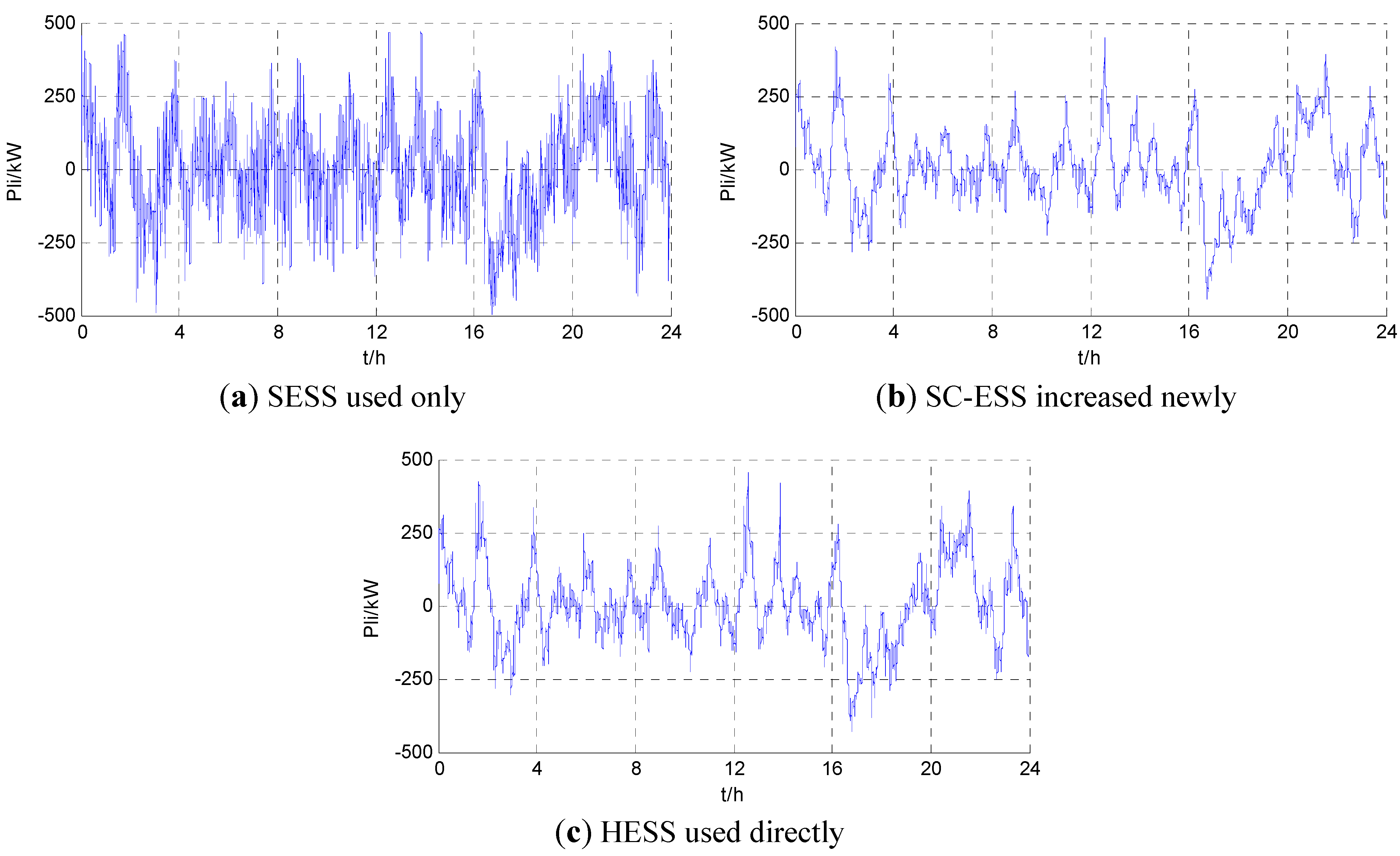
In the practical engineering applications of standalone microgrids for RAPS, ESSs may be configured in three ways. They are SESS used alone, SESS newly increased based on the existing SESS, and HESS used directly. Optimization models aiming at minimizing the total loss equivalent cost of the current ESS are established to comparatively analyze the three application schemes.

5.1. SESS Used Only

When SESS is used, ESS usually adopts an energy-type ESS such as LB-ESS which can be controlled by a Vf pattern. The optimization model of SESS used alone is shown as Equation (32). The parameters to be optimized are P_{r_LB} and E_{r_LB}. The constraint conditions are shown by Equations (27) and (28):

$$\min (C_{opt\_SESS})=\min (C_{loss\_LB}+C_{pen\_ESS})$$

(32)

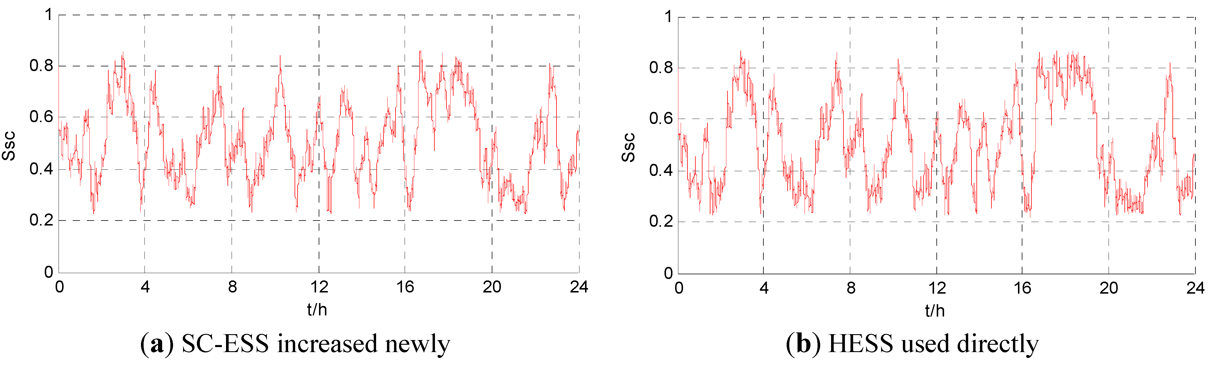
5.2. SC-ESS Increased Newly Based on the Existing SESS

The optimization model of Supercapacitor-Added ESS (SAESS) based on SESS of the existing project is shown by Equation (33). The power rating and storage capacity of LB-ESS are the same as when SESS alone is used, and will not be changed. The parameters to be optimized are P_{r_SC}, E_{r_SC}, T_f0 and ΔS_{co_SC}. The constraint conditions are shown by Equations (27)~(31):

$$\min (C_{opt\_S\text{A}ESS})=\min (C_{loss\_LB}+C_{loss\_SC}+C_{pen\_ESS})$$

(33)

5.3. HESS Used Directly

The optimization model of HESS used directly is shown by Equation (34). The parameters to be optimized are P_{r_LB}, E_{r_LB}, P_{r_SC}, E_{r_SC}, T_f0 and ΔS_{co_SC}. The constraint conditions are shown in Equations (27)~(31):

$$\min (C_{opt\_HESS})=\min (C_{loss\_LB}+C_{loss\_SC}+C_{pen\_ESS})$$

(34)

In addition, as an auxiliary index for analysis, the total initial investment cost of ESSs under the three application schemes is computed using Equations (35), (36) and (37), respectively:

$$C_{total\_SESS}=C_{initial\_LB}$$

(35)

$$C_{total\_SAESS}=C_{total\_SESS}+C_{initial\_SC}$$

(36)

$$C_{total\_HESS}=C_{initial\_LB}+C_{initial\_SC}$$

(37)

6. Case Studies

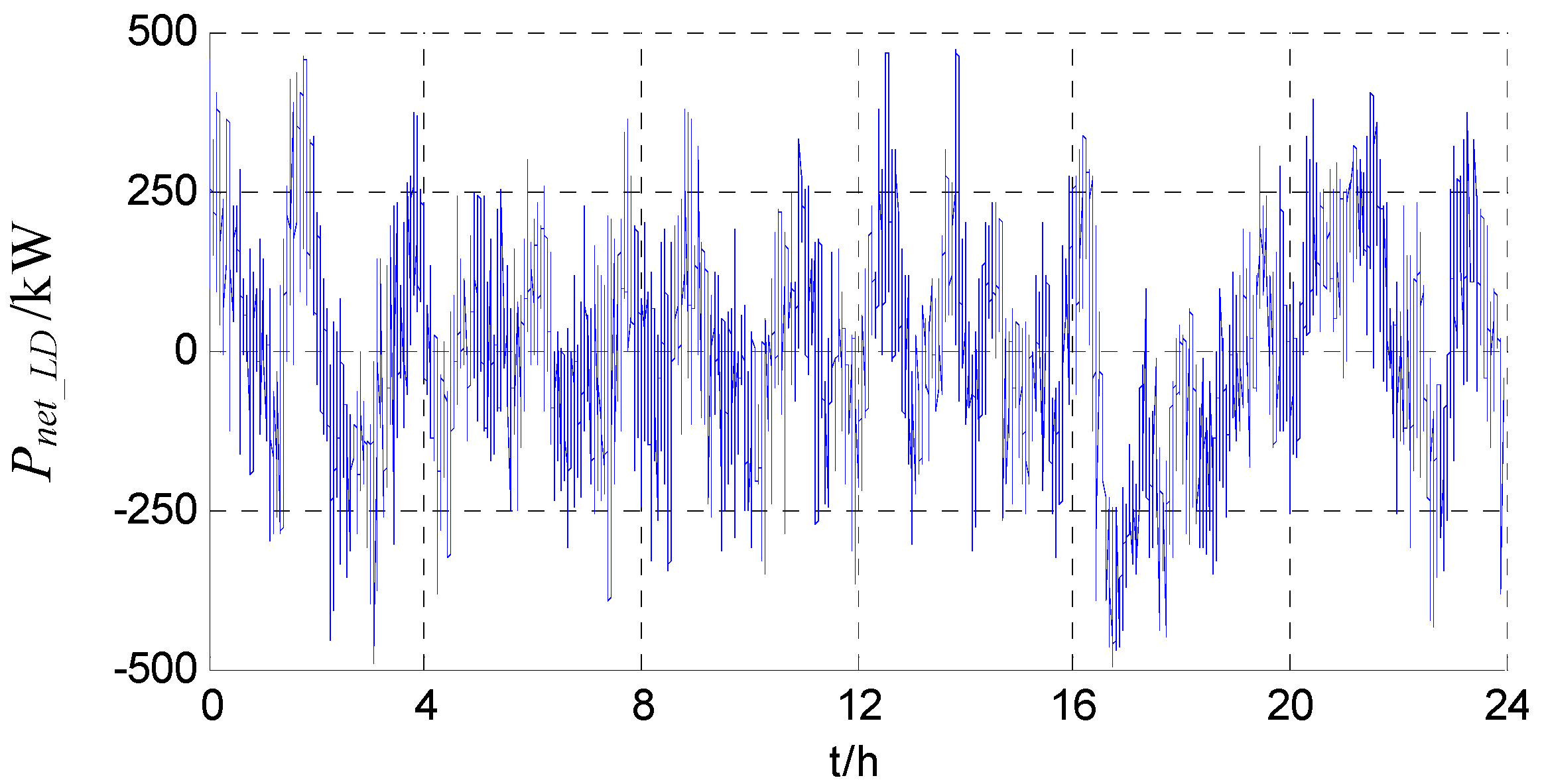
6.1. System Demand and ESS Parameters

The net load curve of one day shown as Figure 5 is the second-level data of field measurements in a standalone microgrid project. The parameters are set as R_set = 99.9%, ΔT_f = 1, F = 10,000$. The main parameters of LB-ESS and SC-ESS are provided in Table 1, where the matching PCSs typically have a lifetime of 10 years, and their initial investment costs are shown in Table 2. A single-stage PCS is used for LB-ESS, and a dual-stage PCS is used for SC-ESS.

Table 1. Main parameters setting of two ESSs.

Parameter type	LB-ESS	SC-ESS
Operating range of SOC	0.25~0.95	0.2~0.9
SOC threshold of over-charge protection	0.9	0.85
SOC threshold of over-discharge protection	0.3	0.25
Initial value of SOC	0.8	0.8
Charge and discharge efficiency	90%	95%
Self-discharge rate (%·s−1)	0	0.00017
Unit capacity cost ($·kWh−1)	655.7	157,377.0

Table 1. Main parameters setting of two ESSs.

Parameter type	LB-ESS	SC-ESS
Operating range of SOC	0.25~0.95	0.2~0.9
SOC threshold of over-charge protection	0.9	0.85
SOC threshold of over-discharge protection	0.3	0.25
Initial value of SOC	0.8	0.8
Charge and discharge efficiency	90%	95%
Self-discharge rate (%·s−1)	0	0.00017
Unit capacity cost ($·kWh−1)	655.7	157,377.0

Table 2. Initial investment cost of the matching PCS for LB-ESS and SC-ESS.

Pr_PCS (kW)	50	100	200	250	300	400	500
CPCS_LB (104·$)	1.00	1.97	3.77	4.61	5.41	6.89	8.20
CPCS_SC (104·$)	1.21	2.36	4.52	5.54	6.49	8.26	9.84

Table 2. Initial investment cost of the matching PCS for LB-ESS and SC-ESS.

Pr_PCS (kW)	50	100	200	250	300	400	500
CPCS_LB (104·$)	1.00	1.97	3.77	4.61	5.41	6.89	8.20
CPCS_SC (104·$)	1.21	2.36	4.52	5.54	6.49	8.26	9.84

Figure 5. Net load curve of the standalone microgrid in one day.

Figure 5. Net load curve of the standalone microgrid in one day.

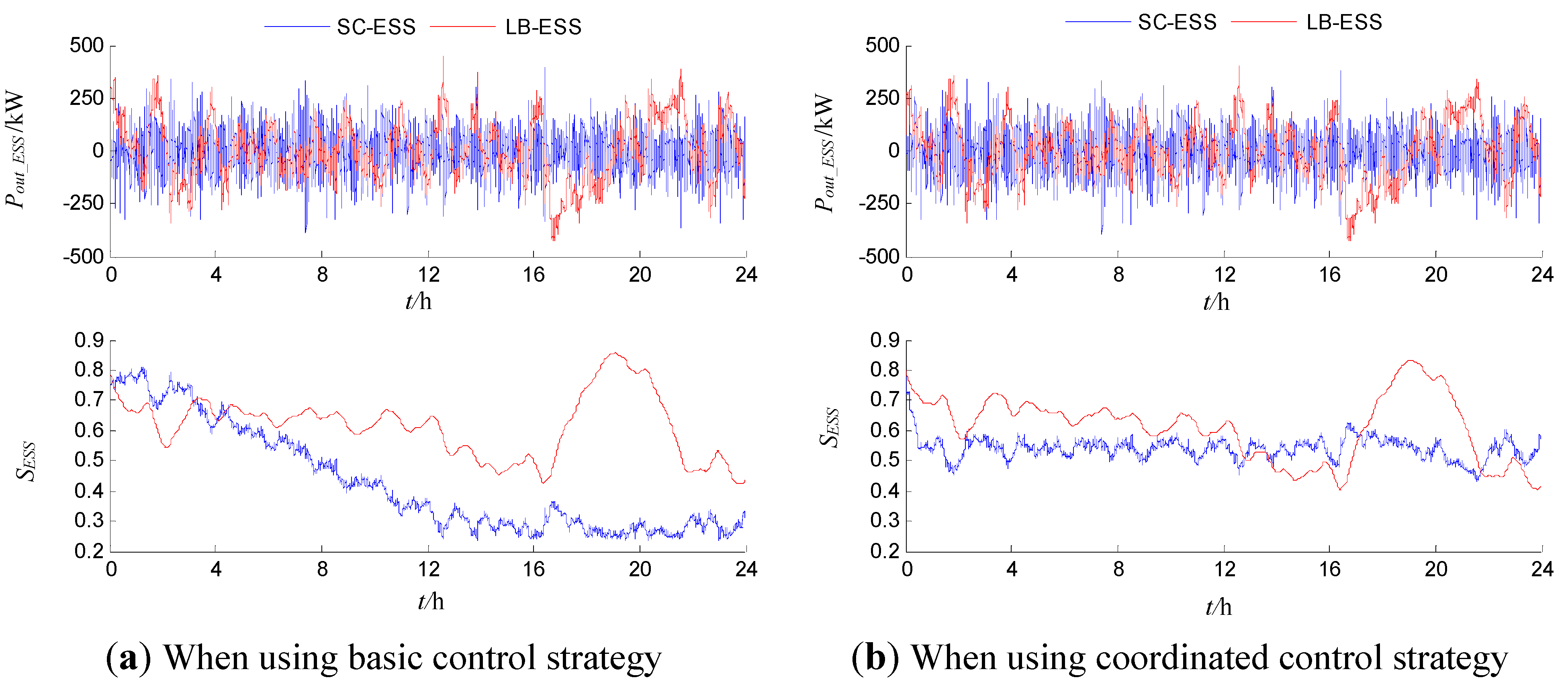
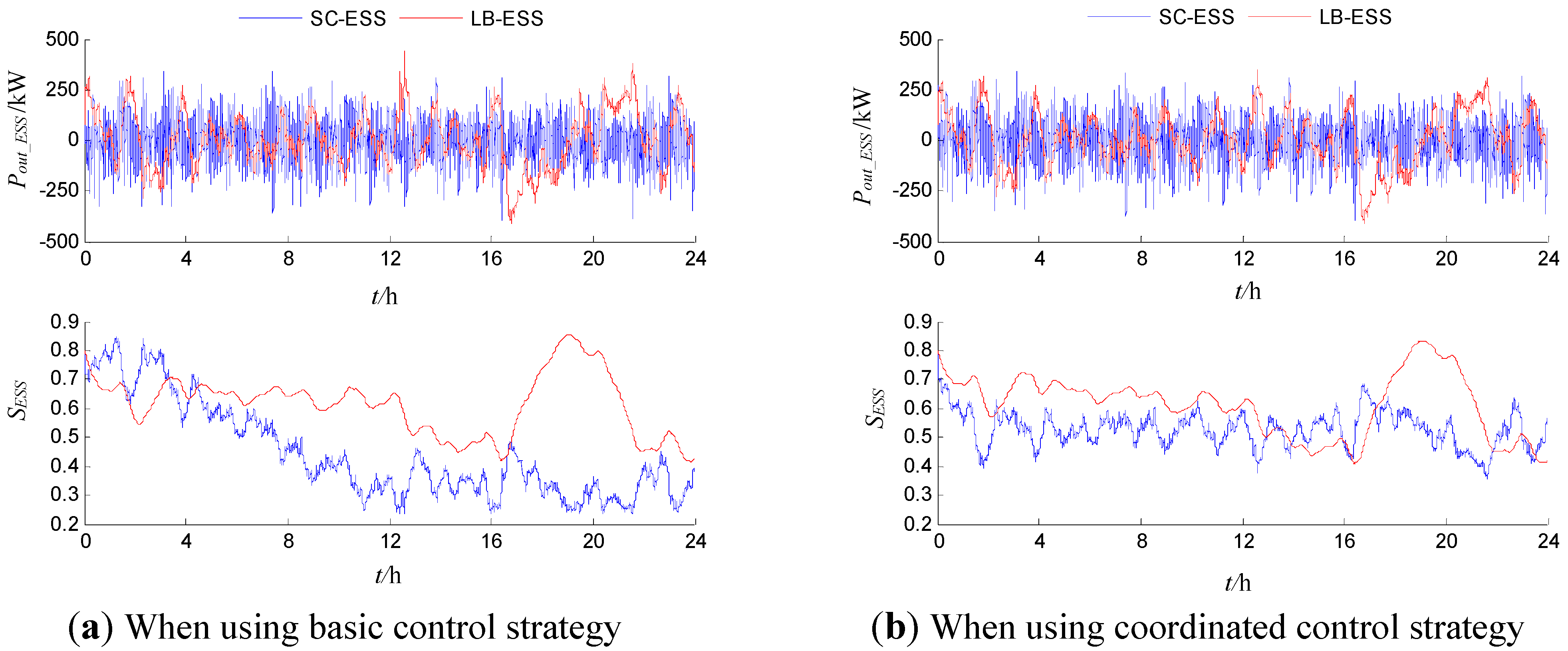
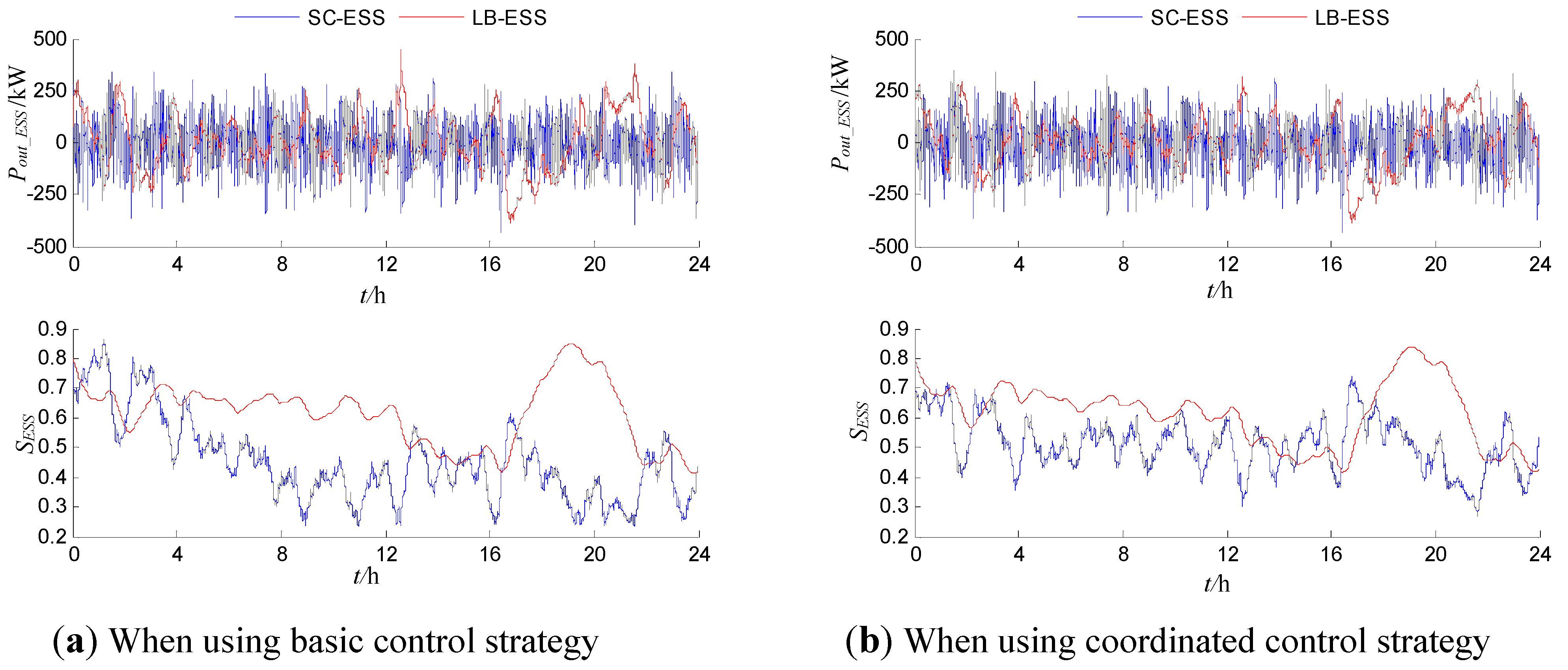
6.2. Comparison of HESS Operation under Different Control Strategies

A case is presented to analyze the difference between the basic control strategy and the coordinated control strategy. Through the comparison of HESS operation under different control strategies, the strategy which will be used for further research can be determined. The operation of HESS using two strategies to satisfy the net load shown in Figure 4 should be compared through the case study. In order to maintain comparability, i.e., the effectiveness of comparative analysis results for different control strategies, the constraint of ESS effective rate should always be fully met. Therefore, HESS should have a redundant configuration based on net load demand. Combined with analysis of Figure 4, the rated output power and rated storage capacity of LB-ESS and SC-ESS are set as 500 kW/1,000 kWh and 500 kW/10 kWh, respectively.

Figure 6. Output power and SOC of two ESSs using two strategies when T_f = 15.

Figure 6. Output power and SOC of two ESSs using two strategies when T_f = 15.

Figure 7. Output power and SOC of two ESSs using two strategies when T_f = 30.

Figure 7. Output power and SOC of two ESSs using two strategies when T_f = 30.

Figure 8. Output power and SOC of two ESSs using two strategies when T_f = 45.

Figure 8. Output power and SOC of two ESSs using two strategies when T_f = 45.

The main control parameters of HESS using the two strategies are T_f0 and ΔS_{co_SC}. The value of ΔS_{co_SC} is set as 0.35 the median of the margin indictor and remains unchanged, because it exists only in the coordinated control strategy. The changes of T_f0 may result in changes of HESS operation under both control strategies. It is necessary to exclude the impact of comparative analysis results of different control strategies by the filter time constant. So the HESS operation curves using different control strategies are given as Figure 6, Figure 7 and Figure 8 when T_f0 is 15, 30 and 45, respectively.

The comparative analysis of Figure 6, Figure 7 and Figure 8 shows that, although there are some differences in the details due to the variation in filter time constant, the variation trends of output power and SOC of LB-ESS and SC-ESS are the same. This conclusion is applicable to both when the basic control strategy is used and the coordinated control strategy is used. No matter which control strategy is used and how much the filter time constant is, the high-frequency parts of power fluctuations are borne by SC-ESS, and the LB-ESS satisfies the remaining non-high-frequency parts. The advantages of different types of ESSs are utilized reasonably.

At the same time, the SOC variation trends of SC-ESS are mainly related to control strategy. For all three cases where filter time constant changes, the SOC of SC-ESS when using the basic control strategy is close to its limit for a long time in the absence of an orderly control. This will result in a significant decrease in their ability to participate in the system power regulation. By contrast, state adjustment of SC-ESS using the coordinated control strategy keeps its SOC in a reasonable range all the time. Through the cooperation between two ESSs, a certain ability to regulate power is always maintained. Therefore, compared with the basic control strategy, the coordinated control strategy has a better performance for HESS operations.

6.3. Comparative Analysis Based on Different Cost and Life Considerations

After determining the HESS control strategy, the comparative analysis of the proposed optimization model and the existing optimization models can be undertaken. With regard to the four different cost and life considerations, the proposed optimization models are solved by a Particle Swarm Optimization (PSO) algorithm. The optimal results are given as Table 3, and the total initial investment cost and total loss equivalent cost of HESS based the corresponding optimal results are given in Table 4.

Table 3. Optimal results of four different considerations in cost and life.

Optimal results	Optimized parameters						Optimized objectives
	Pr_LB (kW)	Er_LB (kWh)	Pr_SC (kW)	Er_SC (kWh)	Tf0 (s)	ΔSco_SC	Cinitial_HESSarr ($)	Cinitial_HESS ($)	Closs_LBarr ($)	Closs_HESS ($)	Cpen_ESS ($)	Copt_HESS ($)
opt1	500	779.4	300	1.73	15	0.52	78.3 × 104	——	——	——	0	78.3 × 104
opt2	500	779.4	300	1.73	15	0.52	——	93.0 × 104	——	——	0	93.0 × 104
opt3	500	749.6	300	5.92	43	0.68	——	——	406.3	——	0	406.3
opt4	500	756.8	300	3.17	24	0.63	——	——	——	467.9	0	467.9

Table 3. Optimal results of four different considerations in cost and life.

Optimal results	Optimized parameters						Optimized objectives
	Pr_LB (kW)	Er_LB (kWh)	Pr_SC (kW)	Er_SC (kWh)	Tf0 (s)	ΔSco_SC	Cinitial_HESSarr ($)	Cinitial_HESS ($)	Closs_LBarr ($)	Closs_HESS ($)	Cpen_ESS ($)	Copt_HESS ($)
opt1	500	779.4	300	1.73	15	0.52	78.3 × 104	——	——	——	0	78.3 × 104
opt2	500	779.4	300	1.73	15	0.52	——	93.0 × 104	——	——	0	93.0 × 104
opt3	500	749.6	300	5.92	43	0.68	——	——	406.3	——	0	406.3
opt4	500	756.8	300	3.17	24	0.63	——	——	——	467.9	0	467.9

Table 4. Comparison of initial investment cost and loss equivalent cost based on optimal results.

Optimalresults	Initial investment cost					Loss equivalent cost
	Carray_LB (104·$)	CPCS_LB (104·$)	Carray_SC (104·$)	CPCS_SC (104·$)	Cinitial_HESS (104·$)	Closs_LBarr ($)	Closs_LB ($)	Closs_SCarr ($)	Closs_SC ($)	Closs_HESS ($)
opt1	51.1	8.2	27.2	6.5	93.0	443.2	465.7	25.2	27.0	492.7
opt2	51.1	8.2	27.2	6.5	93.0	443.2	465.7	25.2	27.0	492.7
opt3	49.2	8.2	93.2	6.5	157.0	406.3	428.7	44.8	46.6	475.3
opt4	49.6	8.2	49.9	6.5	114.2	415.9	438.3	27.8	29.6	467.9

Table 4. Comparison of initial investment cost and loss equivalent cost based on optimal results.

Optimalresults	Initial investment cost					Loss equivalent cost
	Carray_LB (104·$)	CPCS_LB (104·$)	Carray_SC (104·$)	CPCS_SC (104·$)	Cinitial_HESS (104·$)	Closs_LBarr ($)	Closs_LB ($)	Closs_SCarr ($)	Closs_SC ($)	Closs_HESS ($)
opt1	51.1	8.2	27.2	6.5	93.0	443.2	465.7	25.2	27.0	492.7
opt2	51.1	8.2	27.2	6.5	93.0	443.2	465.7	25.2	27.0	492.7
opt3	49.2	8.2	93.2	6.5	157.0	406.3	428.7	44.8	46.6	475.3
opt4	49.6	8.2	49.9	6.5	114.2	415.9	438.3	27.8	29.6	467.9

The analysis combined with the optimization results in Table 3 and Table 4 shows that:

• The initial investment cost of HESS is optimized in both Objective 1 and Objective 2, and the difference is whether to consider the cost of matched PCS. The optimized results are the same for both objectives, because PCSs in practical engineering applications are usually standard equipment packages. The rated output power of PCS has only a few optional specification values. This characteristic of non-continuous changes makes the initial investment cost of matched PCS relatively fixed. However, if this part of the cost has not counted in the project budget, a poor decision will be made. For example, an additional expense of 0.147 million dollars will be produced in this case study. Therefore, to minimize the amount of capital in initial investment of HESS, optimization using Objective 2 is more reasonable.
• The data comparing optimization when using Objective 2, Objective 3 and Objective 4 is analyzed to obtain the differences between minimizing the initial investment cost and minimizing the loss equivalent cost. The initial investment cost of whole HESS when using Objective 2 is 0.930 million dollars, which is 0.640 million dollars lower than using Objective 3 with a decline of 40.75%, and 0.212 million dollars lower than using Objective 4 with a decline of 18.55%. At the same time, the total loss equivalent cost of HESS when using Objective 2 is 492.7 dollars, which is 17.4 dollars more than using Objective 3 with an increase of 3.67%, and 24.8 dollars more than using Objective 4 with an increase of 5.29%. Compared with the cost when optimizing the loss equivalent cost, although the initial investment cost of whole HESS when optimizing the initial investment cost is lower, the total loss equivalent cost of HESS per unit time is significantly higher. As a result, from the point of life cycle cost, the overall performance of HESS is better when optimizing the loss equivalent cost.
• The life loss and cost conversion of storage arrays in LB-ESS are considered in Objective 3, and the life loss and cost conversion of whole HESS are considered in Objective 4. The life of storage arrays in LB-ESS is much less than the life of other components in HESS, so it is the main factor in HESS performance. As shown in Table 4, the minimum total loss equivalent cost of HESS is 467.9 dollars, i.e., the result when using Objective 4. When using Objective 3, the total loss equivalent cost of HESS is 475.3 dollars, which is only 7.3 dollars more than the optimal value with a difference of 1.57%. That is to say that, an approximately optimal value is obtained when using Objective 3. Meanwhile, the loss equivalent cost of storage arrays in LB-ESS is lowest when using Objective 3, which is 9.6 dollars lower than when using Objective 4 with a decline of 2.32%. The initial investment cost of whole HESS when using Objective 3 is 0.428 million dollars more than when using Objective 4 with an increase of 37.48%. Hence, the economic cost when using Objective 3 is difficult to accept, although the loss equivalent cost of storage arrays in LB-ESS can be lowest and an approximate minimum of total loss equivalent cost of HESS can be obtained.

In summary, taking the total loss equivalent cost of HESS as optimization objective is best. The technical and economic characteristics of HESS will be optimal only when the life quantification and cost conversion of all storage arrays and matched PCSs are taken into account. When considering storage arrays only, there will be a poor decision of initial investment in the project budget and an approximate optimal result of HESS overall performance. Although the optimization of HESS overall technical and economic characteristics is very important, the optimization of HESS initial investment is also important especially when considering capital as a decision-making factor in the project.

6.4. Comparative Analysis Based on Different ESS Application Schemes

Through the analysis for the same scheme of ESS application in Section 6.3, the overall optimization can be achieved only when the technical and economic impact of all devices in HESS are considered. In the practical engineering, there are some different ESS application schemes. The comparative analysis based on the different application schemes of ESSs are discussed in this section. For the three schemes of SESS used alone, SC-ESS newly increased and HESS used directly, the proposed optimization models are solved by the PSO algorithm, and the optimal results are given as follows.

Table 5. Optimization results of ESSs in three schemes.

Optimal results	Optimized parameters						Loss equivalent cost			Initial investment cost
	Pr_LB (kW)	Er_LB (kWh)	Pr_SC (kW)	Er_SC (kWh)	Tf0 (s)	ΔSco_SC	Closs_LB ($)	Closs_SC ($)	Closs_HESS ($)	Cinitial_LB (104·$)	Cinitial_SC (104·$)	Cinitial_HESS (104·$)
SESS used only	500	781.5	——	——	——	——	577.7	——	577.7	59.4	——	59.4
SC-ESS increased newly	——	——	300	3.58	28	0.54	456.7	30.6	487.4	——	62.8	122.3
HESS used directly	500	756.8	300	3.17	24	0.63	438.3	29.6	467.9	57.8	56.4	114.2

Table 5. Optimization results of ESSs in three schemes.

Optimal results	Optimized parameters						Loss equivalent cost			Initial investment cost
	Pr_LB (kW)	Er_LB (kWh)	Pr_SC (kW)	Er_SC (kWh)	Tf0 (s)	ΔSco_SC	Closs_LB ($)	Closs_SC ($)	Closs_HESS ($)	Cinitial_LB (104·$)	Cinitial_SC (104·$)	Cinitial_HESS (104·$)
SESS used only	500	781.5	——	——	——	——	577.7	——	577.7	59.4	——	59.4
SC-ESS increased newly	——	——	300	3.58	28	0.54	456.7	30.6	487.4	——	62.8	122.3
HESS used directly	500	756.8	300	3.17	24	0.63	438.3	29.6	467.9	57.8	56.4	114.2

The analysis based on the sheet data above shows that:

• As shown in the optimal results of the three schemes, the loss equivalent cost of LB-ESS is 577.7, 456.7 and 438.3 dollars, respectively. Compared with the loss equivalent cost of LB-ESS when SESS is used alone, this cost is decreased by 20.9% when SC-ESS is newly increased, and decreased by 24.1% when HESS is used directly. The data analysis above shows that, compared with SESS used alone, the utilization of SC-ESS can effectively reduce the life loss equivalent cost of LB-ESS.
• Compared with SESS used alone, an additional initial investment cost of 0.628 million dollars is needed after SC-ESS is newly increased. However, the total loss equivalent cost of HESS in the simulation time is reduced from 577.7 dollars to 487.4 dollars, which is decreased by 15.6% based on the cost of SESS. This indicates that the initial investment cost is increased because of a newly increased SC-ESS, but the total loss of ESSs demanded by a standalone microgrid is effectively reduced in unit time, so the technical and economic characteristics are much better than SESS.
• After overall optimization of HESS used directly, the total loss equivalent cost has been decreased to 467.9 dollars, which represents a significant decreased amplitude of 19.0% compared with SESS used alone. In addition, compared with optimization of SC-ESS increased newly, the overall optimization of HESS used results in a decrease of the total initial investment cost from 1.223 to 1.142 million dollars, i.e., a savings 80.7 thousand dollars in the initial investment cost. Therefore, the technical and economic characteristics have a further enhance after overall optimization of HESS used directly.

Meanwhile, combined with the optimal results in Table 3, output power curves and SOC curves of various ESSs in three schemes are shown as follows.

Figure 9. The output power curves of LB-ESS in the three schemes.

Figure 9. The output power curves of LB-ESS in the three schemes.

Figure 10. The SOC curves of LB-ESS in the three schemes.

Figure 10. The SOC curves of LB-ESS in the three schemes.

Figure 11. The output power curves of SC-ESS in the latter two schemes.

Figure 11. The output power curves of SC-ESS in the latter two schemes.

Figure 12. The SOC curves of SC-ESS in the latter two schemes.

Figure 12. The SOC curves of SC-ESS in the latter two schemes.

As shown in Figure 9, Figure 10, Figure 11 and Figure 12, the output power and SOC of each ESS in the three schemes are all close to the permitted upper and lower limits of normal operation. By contrast, the output power and SOC of ESSs given in Figure 6, Figure 7 and Figure 8 above can’t do it, especially the SOC curves of SC-ESS. In other words, the required performances of this application mode have been achieved by minimum power rating and minimum storage capacity of the ESSs after optimization of the three schemes. The advantages of technical complementary characteristics between energy-type energy storage and power-type energy storage are given full play in the latter two schemes, and optimal configuration and operation of the whole ESSs is achieved. Therefore, the scheme parameter combinations of this day as shown in Table 3 can be accepted as optimal in a more intuitive expression.

7. Conclusions

A new index named ESS efficiency rate is proposed in this paper considering the characteristics of a small-scale standalone microgrid for RAPS. The index reflects the common satisfaction of load demands and maximized utilization of renewable energy. Compared with LOLP or LPSP, ESS efficiency rate is more suitable as the constraint condition of ESS optimization analysis model in the microgrid. At the same time, the second-level data of field measurement is used in optimization instead of hour-level data making the analysis results more credible. Because the real time curves of output power and SOC of SC-ESS can be obtained, although the duration of SC-ESS continuous discharge at rate power is very short.

With regard to the operating control of HESS, the coordinated control strategy based on state cooperation is based on the basic control strategy considering power allocation only. The increased measures in coordinated control strategy are status adjustment of SC-ESS, coordination of overcharge and over-discharge protection, and coordination of maximum power limit protection. A numerical example shows that, for different filter time constants, the power adjustment abilities of SC-ESS when using coordinated control strategy are all significantly better than when using the basic control strategy.

Three different optimization objective functions are established in the optimization of HESS. The impact of incomplete consideration of cost and life on overall performance of HESS is comparatively analyzed. A numerical example shows that the cost of matched PCSs must be taken in account in the optimization. Although the initial investment cost of HESS can be reduced when taking one-time investment cost as optimization objective, the usage cost per unit time is unacceptable and the optimized results when taking the loss equivalent cost of LB storage arrays as optimization objective are approximately optimal. Only when considering the life quantification and cost equivalent of the whole HESS, the optimized results can get the best technical and economic characteristics of HESS.

The different application schemes of ESS in practical projects are contrastively analyzed. The analysis results show that, although the initial investment cost of SC-ESS increased newly based on SESS increases, the total loss equivalent cost of ESSs in unit time decreases significantly. If HESS is used directly, the total loss equivalent cost of ESSs can be further reduced. The ESS characteristics of practical projects are considered, such as self-discharge of ESSs, PCSs to be standard equipment packages, and so on. The analysis results have guiding significance and provide reference values for ESS applications in existing and new projects.

References

1. Mendis, N.; Muttaqi, K.M.; Perera, S. Management of low- and high-frequency power components in demand-generation fluctuations of a DFIG-based wind-dominated RAPS system using hybrid energy storage. IEEE Trans. Ind. Appl. 2014, 50, 2258–2268. [Google Scholar] [CrossRef]
2. Moseley, P.T. Energy storage in remote area power supply (RAPS) systems. J. Power Sources 2006, 155, 83–87. [Google Scholar] [CrossRef]
3. Dragicevic, T.; Guerrero, J.M.; Vasquez, J.C. A distributed control strategy for coordination of an autonomous LVDC microgrid based on power-line signalling. IEEE Trans. Ind. Electron. 2014, 61, 3313–3326. [Google Scholar] [CrossRef]
4. Wu, D.; Tang, F.; Dragicevic, T.; Vasquez, J.C.; Guerrero, J.M. Autonomous active power control for islanded AC microgrids with photovoltaic generation and energy storage system. IEEE Trans. Energy Convers. 2014, 29, 882–892. [Google Scholar] [CrossRef]
5. Dragicevic, T.; Pandzic, H.; Skrlec, D.; Kuzle, I.; Guerrero, J.M.; Kirschen, D.S. Capacity optimization of renewable energy sources and battery storage in an autonomous telecommunication facility. IEEE Trans. Sustain. Energy 2014, 5, 1367–1378. [Google Scholar] [CrossRef]
6. Kim, J.Y.; Kim, H.M.; Kim, S.K.; Jeon, J.H.; Choi, H.K. Designing an energy storage system fuzzy PID controller for microgrid islanded operation. Energies 2011, 4, 1443–1460. [Google Scholar] [CrossRef]
7. Li, J.; Wei, W.; Xiang, J. A simple sizing algorithm for stand-alone PV/Wind/Battery hybrid microgrids. Energies 2012, 5, 5307–5323. [Google Scholar] [CrossRef]
8. Marzband, M.; Sumper, A.; Ruiz-Alvarez, A.; Dominguez-Garcia, J.L.; Tomoiaga, B. Experimental evaluation of a real time energy management system for stand-alone microgrids in day-ahead markets. Appl. Energy 2013, 106, 365–376. [Google Scholar] [CrossRef]
9. Marzband, M.; Sumper, A.; Dominguez-Garcia, J.L.; Gumara-Ferret, R. Experimental Validation of a Real Time Energy Management System for Microgrids in Islanded Mode Using a Local Day-Ahead Electricity Market and MINLP. Energy Convers. Manag. 2013, 76, 314–322. [Google Scholar] [CrossRef]
10. Marzband, M.; Ghadimi, M.; Sumper, A.; Dominguez-Garcia, J.L. Experimental validation of a real-time energy management system using multi-period gravitational search algorithm for microgrids in islanded mode. Appl. Energy 2014, 128, 164–174. [Google Scholar] [CrossRef] [Green Version]
11. Gao, L.; Dougal, R.A.; Liu, S. Power enhancement of an actively controlled battery/ultracapacitor hybrid. IEEE Trans. Power Electron. 2005, 20, 236–243. [Google Scholar] [CrossRef]
12. Dougal, R.A.; Liu, S.; White, R.E. Power and life extension of battery ultracapacitor hybrids. IEEE Trans. Components Packag. Technol. 2002, 25, 120–131. [Google Scholar] [CrossRef]
13. Li, W.; Joos, G.; Belanger, J. Real-time simulation of a wind turbine generator coupled with a battery supercapacitor energy storage system. IEEE Trans. Ind. Electron. 2010, 57, 1137–1145. [Google Scholar] [CrossRef]
14. Thounthong, P.; Rael, S.; Davat, B. Control strategy of fuel cell and supercapacitors association for a distributed generation system. IEEE Trans. Ind. Electron. 2007, 54, 3225–3233. [Google Scholar] [CrossRef]
15. Gee, A.M.; Roninson, F.V.P.; Dunn, R.W. Analysis of battery lifetime extension in a small-scale wind-energy system using supercapacitors. IEEE Trans. Energy Convers. 2013, 28, 24–33. [Google Scholar] [CrossRef]
16. Mendis, N.; Muttaqi, K.M.; Perera, S. Management of battery-supercapacitor hybrid energy storage and synchronous condenser for isolated operation of PMSM based variable-speed wind turbine generating systems. IEEE Trans. Smart Grid 2014, 5, 944–953. [Google Scholar] [CrossRef]
17. Xue, F.; Gooi, H.B.; Chen, S. Hybrid energy storage with multimode fuzzy power allocator for PV systems. IEEE Trans. Sustain. Energy 2014, 5, 389–397. [Google Scholar] [CrossRef]
18. Singo, T.A.; Martinez, A.; Saadate, S. Design and implementation of a photovoltaic system using hybrid energy storage. In Proceedings of the IEEE 11th International Conference on Optimization of Electrical and Electronic Equipment, Brasov, Romania, 22–24 May 2008.
19. Li, C.; Yang, X.; Zhang, M.; Wang, H.; Ye, J.; Chen, J. Optimal configuration scheme for hybrid energy storage system of super-capacitors and batteries based on cost analysis. Autom. Electr. Power Syst. 2013, 37, 1–5. [Google Scholar]
20. Tian, P.; Xiao, X.; Ding, R.; Huang, X. A capacity configuring method of composite energy storage system in autonomous multi-microgrid. Autom. Electr. Power Syst. 2013, 37, 168–173. [Google Scholar]
21. Zhou, T.; Sun, W. Optimization of battery-supercapacitor hybrid energy storage station in wind/solar generation system. IEEE Trans. Sustain. Energy 2014, 5, 408–415. [Google Scholar] [CrossRef]
22. Glavin, M.E.; Chan, P.K.W.; Hurley, W.G. Optimization of autonomous hybrid energy storage system for photovoltaic application. In Proceedings of the Energy Conversion Congress and Exposition, San Jose, CA, USA, 20–24 September 2009.
23. Etinski, M.; Schulke, A. Optimal hybrid energy storage for wind energy integration. In Proceedings of the IEEE International Conference on Industrial Technology (ICIT), Cape Town, South Africa, 25–28 February 2013.
24. Yu, W.; Liu, D.; Huang, Y. Operation optimization based on the power supply and storage capacity of an active distribution network. Energies 2013, 6, 6423–6438. [Google Scholar] [CrossRef]
25. Wee, K.W.; Choi, S.S.; Vilathgamuwa, D.M. Design of a least-cost battery-supercapacitor energy storage system for realizing dispatchable wind power. IEEE Tans. Sustain. Energy 2013, 4, 786–796. [Google Scholar] [CrossRef]
26. Sen, C.; Usama, Y.; Carciumaru, T.; Lu, X.; Kar, N.C. Design of a novel wavelet based transient detection unit for in-vehicle fault determination and hybrid energy storage utilization. IEEE Trans. Smart Grid 2012, 3, 422–433. [Google Scholar] [CrossRef]
27. Jiang, Q.; Hong, H. Wavelet-based capacity configuration and coordinated control of hybrid energy storage system for smoothing out wind power fluctuations. IEEE Trans. Power Syst. 2013, 28, 1363–1372. [Google Scholar] [CrossRef]
28. Kazempour, S.J.; Moghaddam, M.P.; Haghifam, M.R.; Yousefi, G.R. Electric energy storage systems in a market-based economy: Comparison of emerging and traditional technologies. Renew. Energy 2009, 34, 2630–2639. [Google Scholar] [CrossRef]
29. Nguyen, M.Y.; Nguyen, D.H.; Yoon, Y.T. A new battery energy storage charging/discharging scheme for wind power producers in real-time markets. Energies 2012, 5, 5439–5452. [Google Scholar] [CrossRef]
30. Yang, W.; Wang, X.; Li, X.; Liu, Z. An active power sharing method among distributed energy sources in an islanded series micro-grid. Energies 2014, 7, 7878–7892. [Google Scholar] [CrossRef]
31. Li, F.; Xie, K.; Zhang, X.; Wang, K.; Zhou, D.; Zhao, B. Design of control strategy for hybrid energy storage system based on charge-discharge state of lithium battery. Autom. Electr. Power Syst. 2013, 37, 70–75. [Google Scholar]
32. Li, F.; Xie, K.; Zhang, X.; Zhao, B.; Chen, J. Optimization of coordinated control parameters for hybrid energy storage system based on life quantization. Autom. Electr. Power Syst. 2014, 38, 1–5. [Google Scholar]
33. Millner, A. Modeling lithium ion battery degradation in electric vehicles. In Proceedings of the IEEE Conference on Innovative Technologies for an Efficient and Reliable Electricity Supply (CITRES), Waltham, MA, USA, 27–29 September 2010.
34. Xie, Q.; Lin, X.; Wang, Y.; Pedram, M.; Shin, D.; Chang, N. State of health aware charge management in hybrid electrical energy storage systems. In Proceedings of the Design, Automation & Test in Europe Conference & Exhibition (DATE), Dresden, Germany, 12–16 March 2012.
35. Xie, Q.; Yue, S.; Pedram, M.; Shin, D.; Chang, N. Adaptive thermal management for portable system batteries by forced convection cooling. In Proceedings of the Design, Automation & Test in Europe Conference & Exhibition (DATE), 18–22 March 2013.
36. Lam, L.; Bauer, P. Practical capacity fading model for Li-ion battery cells in electric vehicles. IEEE Trans. Power Electron. 2013, 28, 5910–5918. [Google Scholar] [CrossRef]
37. Vergara, C.R. Parametric interface for battery energy storage systems providing ancillary services. In Proceedings of the 3rd IEEE PES International Conference and Exhibition on Innovative Smart Grid Technologies (ISGT Europe), 14–17 October 2012.
38. Traube, J.; Lu, F.; Maksimovic, D.; Mossoba, J.; Kromer, M.; Faill, P.; Katz, S.; Borowy, B.; Nichols, S.; Casey, L. Mitigation of solar irradiance intermittency in photovoltaic power systems with integrated electric-vehicle charging functionality. IEEE Trans. Power Electron. 2013, 28, 3058–3067. [Google Scholar] [CrossRef]
39. Grahn, P.; Munkhammar, J.; Widen, J.; Alvehag, K.; Soder, L. PHEV home-charging model based on residential activity patterns. IEEE Trans. Power Syst. 2013, 28, 2507–2515. [Google Scholar] [CrossRef]
40. Xie, Q.; Wang, Y.; Kim, Y.; Pedram, M.; Chang, N. Charge allocation in hybrid electrical energy storage systems. IEEE Trans. Comput. Aided Des. Integr. Circuits Syst. 2013, 32, 1003–1016. [Google Scholar] [CrossRef]
41. Onar, O.C.; Khaligh, A. A novel integrated magnetic structure based DC/DC converter for hybrid battery/ultracapacitor energy storage systems. IEEE Trans. Smart Grid 2012, 3, 296–307. [Google Scholar] [CrossRef]