Application of a Central Composite Design for the Study of NO_x Emission Performance of a Low NO_x Burner

Abstract

In this study, the influence of various factors on nitrogen oxides (NO_x) emissions of a low NO_x burner is investigated using a central composite design (CCD) approach to an experimental matrix in order to show the applicability of design of experiments methodology to the combustion field. Four factors have been analyzed in terms of their impact on NO_x formation: hydrogen fraction in the fuel (0%–15% mass fraction in hydrogen-enriched methane), amount of excess air (5%–30%), burner head position (20–25 mm from the burner throat) and secondary fuel fraction provided to the burner (0%–6%). The measurements were performed at a constant thermal load equal to 25 kW (calculated based on lower heating value). Response surface methodology and CCD were used to develop a second-degree polynomial regression model of the burner NO_x emissions. The significance of the tested factors over their respective ranges has been evaluated using the analysis of variance and by the consideration of the coefficients of the model equation. Results show that hydrogen addition to methane leads to increased NO_x emissions in comparison to emissions from pure methane combustion. Hydrogen content in a fuel is the strongest factor affecting NO_x emissions among all the factors tested. Lower NO_x formation because of increased excess air was observed when the burner was fuelled by pure methane, but this effect diminished for hydrogen-rich fuel mixtures. NO_x emissions were slightly reduced when the burner head was shifted closer to the burner outer tube, whereas a secondary fuel stream provided to the burner was found to have no impact on NO_x emissions over the investigated range of factors.

1. Introduction

The latest trends in environmental legislation associated with carbon dioxide (CO₂) emission reductions are a great challenge for the industrial sector. It can be assumed that a competitive position for businesses utilizing fossil fuels will be strongly conditioned on the ability to meet strict environmental regulations. Therefore, the necessity of reducing CO₂ emissions has led to the development of various technological solutions, called carbon capture and storage technologies. One of these technologies is associated with hydrogen or hydrogen-enriched fuel combustion. The pre-combustion CO₂ capture technology can be applied to power plants, but also to industrial processes as in refineries [1,2,3]. In this case, the fossil fuel is processed by gasification or reforming and water-gas shift reaction to generate a fuel composed mainly of hydrogen and CO₂. CO₂ is then captured leaving a hydrogen-rich fuel, what allows for CO₂ emission reduction. However, the use of such fuels in engineering applications is associated with corresponding changes in nitrogen oxides (NO_x) emissions, which in turn are affected by many factors.

In both science and engineering, determining which factors of a complex system are significant and how they affect the response of the system is often difficult. In such cases, usually full factorial design of the experiment is used to test all possible combinations of various factors. Full factorial design is often the only choice when one is interested in accurate measurement results under various operating conditions or when the response is expected to change in unforeseen ways. Note that this approach often requires a large number of experimental trials, because the number of trials increases geometrically with the number of factors to be tested. Furthermore, the interpretation of a large set of measurement data is difficult and may be unnecessary, because especially in engineering and practical applications, focus on only trends in how factors affect system response can be sufficient. Therefore, response surface methodology combined with central composite design (CCD) [4] is an efficient technique for experimentally exploring relationships between investigated factors and system response.

Most practical industrial burner designs are much more sophisticated combustion systems than those used in the scientific investigations of combustion processes. Many factors may affect pollutant emissions from these burners, while in cases of high-burner thermal power, conducting measurements in such industrial facilities is often difficult and expensive [5]. Statistically cognizant design of experiment facilitates an understanding of the influence of the factors tested and the interactions between these factors on system response by using a minimum number of experimental trials. Such an approach applied to testing of burners might be also helpful in reducing the costs of large industrial scale experiments.

The purpose of this paper is to present the use of the high performance and predictive strength of CCD to study NO_x emissions from a Partially Premixed Bluff Body (PPBB) burner. The PPBB burner was chosen because it allows testing several factors including fuel composition, excess air, fuel distribution method and the factor that determines burner geometry. Understanding the influence of these factors on NO_x emissions is considerably important for burner development.

2. PPBB Burner

Bluff body stabilized flames have been an important research topic for a long time, mainly because of the fact that some form of flame stabilization is often required in industrial applications. When bluff body is used as a flame holder, the incoming fuel and oxidizer mixture is ignited by the hot combustion products recirculating in a wake structure formed behind the bluff body. This stabilization mechanism has been investigated extensively by many researchers [6,7,8,9,10,11,12]. Many studies associated with bluff body stabilization mechanism focus on premixed combustion systems, where premixed fuel and oxidizer are provided to the combustion zone and thus complex physics that controls mixing process can be neglected. However, it is worth noting that premixed combustion systems may suffer from flashback phenomena, what in turn can lead to burner damage and it may have potentially dangerous consequences, especially in industrial applications. Risk of flashback can be eliminated by using partially premixed flames.

The PPBB burner described in Figure 1 functions by partially mixing the fuel with air rapidly and stabilizing the flame by a bluff body. The air flow is suddenly accelerated when approaching the burner exit section, also called burner throat, because of the progressively reduced cross section formed between the diverging burner head and the outer tube. Gaseous fuel is distributed from the burner head, i.e., fuel lance, in the accelerating air flow and is partially mixed with air before stabilization. A flame stabilization zone is created at the front of the lance by recirculation initiated by the shape of the lance, as shown in Figure 2.

Figure 1. Schematic representation of the test rig and the PPBB burner used in the experiments (dimensions in mm).

Figure 1. Schematic representation of the test rig and the PPBB burner used in the experiments (dimensions in mm).

Figure 2. Photography of hydrogen-enriched methane flame stabilized behind the lance of the PPBB burner.

Figure 2. Photography of hydrogen-enriched methane flame stabilized behind the lance of the PPBB burner.

The PPBB burner design allows for controlling the combustion process using two design parameters for a given fuel composition. The first parameter is the distance between the lance and the burner exit section (labelled X3 in Figure 1). The distance can be changed by moving the fuel lance relative to the burner throat section. The lance position determines the point of fuel injection into the accelerated air, relative to the outer tube, and affects the fuel and air mixing process. The fuel distribution method is the second parameter affecting burner operation. Fuel provided to the burner is divided into a primary fuel stream selectively distributed from ports at the bottom of the lance and a secondary fuel stream from ports arranged around at the top of the lance. The fuel distribution method affects gas composition in the reaction zone. Consequently, it can be stated that the design parameters control mixing process in the burner, which involves changes of flow pattern behind the lance, fuel jets-air stream interaction and primary fuel jet-secondary fuel jet interactions. These phenomena may have significant impact on NO_x emissions and flame stability [13,14].

3. Central Composite Design of the Experiment

CCD enables estimation of the regression parameters to fit a second-degree polynomial regression model to a given response. A polynomial, as given by Equation (1), quantifies relationships among the measured response y and a number of experimental variables X₁…X_k, where k is the number of factors considered, β are regressors and ε is an error associated with the model:

$$\begin{array}{l}y={\mathrm{\beta }}_0+{\mathrm{\beta }}_1{X}_1+{\mathrm{\beta }}_2{X}_2+\dots +{\mathrm{\beta }}_k{X}_k\\ +{\mathrm{\beta }}_{11}{X}_1^2+{\mathrm{\beta }}_{22}{X}_2^2+\dots +{\mathrm{\beta }}_{kk}{X}_k^2\\ +{\mathrm{\beta }}_{12}{X}_1{X}_2+\dots +{\mathrm{\beta }}_{k-1,k}{X}_{k-1}{X}_k+\mathrm{\epsilon }\end{array}$$

(1)

The regressors (β₁, β₂, β₃…) in the various terms of Equation (1) provide a quantitative measure of the significance of linear effects, curvilinear effects of factors and interactions between factors. It is worth noting that the model presented by Equation (1) is not a model in purely physical sense, but rather it should be understood as a statistical model, i.e., a correlation developed based on regression analysis. However, this nomenclature is widely used in the field of design of experiments and statistics, and therefore it is used hereafter.

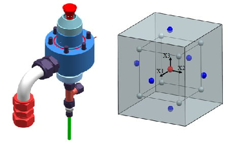
CCD requires three types of trials, i.e., 2^k factorial trials, 2k axial trials and n_c center point trials, where k is number of factors studied in the experiment [15]. As an example, this is illustrated in Figure 3, where each point defines a unique set of values of experimental trials for the three factors (k = 3) tested in an experiment.

Figure 3. Visualization of original type rotatable CCD for three factors: X1, X2 and X3.

Figure 3. Visualization of original type rotatable CCD for three factors: X1, X2 and X3.

Values at the center point (red point with coordinates 0, 0, 0) that is located in the center of the cube are used to detect curvature in the response, i.e., they contribute to the estimation of the coefficients of quadratic terms. Axial points (six blue points located at a distance α from the center point) are also used to estimate the coefficients of quadratic terms, while factorial points (eight grey points located at corners of the cube with a side length equal to 2) are used mainly to estimate the coefficients of linear terms and two-way interactions. For testing four or more factors in an experiment, Figure 3 should be extended to the fourth or more dimensions.

In CCD, factors are tested at a minimum of three levels: minimum, middle and maximum, equivalent to levels −1, 0 and 1, which are called coded units. If X_min and X_max are respectively minimum and maximum absolute, i.e., uncoded, values of a factor, the absolute values X corresponding the respective coded values can be obtained by a simple linear transformation of the original measurement scale, namely:

$$X=b\cdot codedvalue+a$$

(2)

where:

$$a=\frac{X_{\max }+X_{\min }}{2},b=\frac{X_{\max }-X_{\min }}{2}$$

(3)

To obtain the rotatability of a design, each experimental factor must be represented at the five levels of coded units: −α, −1, 0, 1, α. This property ensures constant variance at points that are equidistant from the center point, and therefore provides equal precision of response estimation in any direction of the design. For a full factorial CCD, it can be shown [16] that a design is rotatable if:

$$\mathrm{\alpha }={\left(2^k\right)}^{0.25}$$

(4)

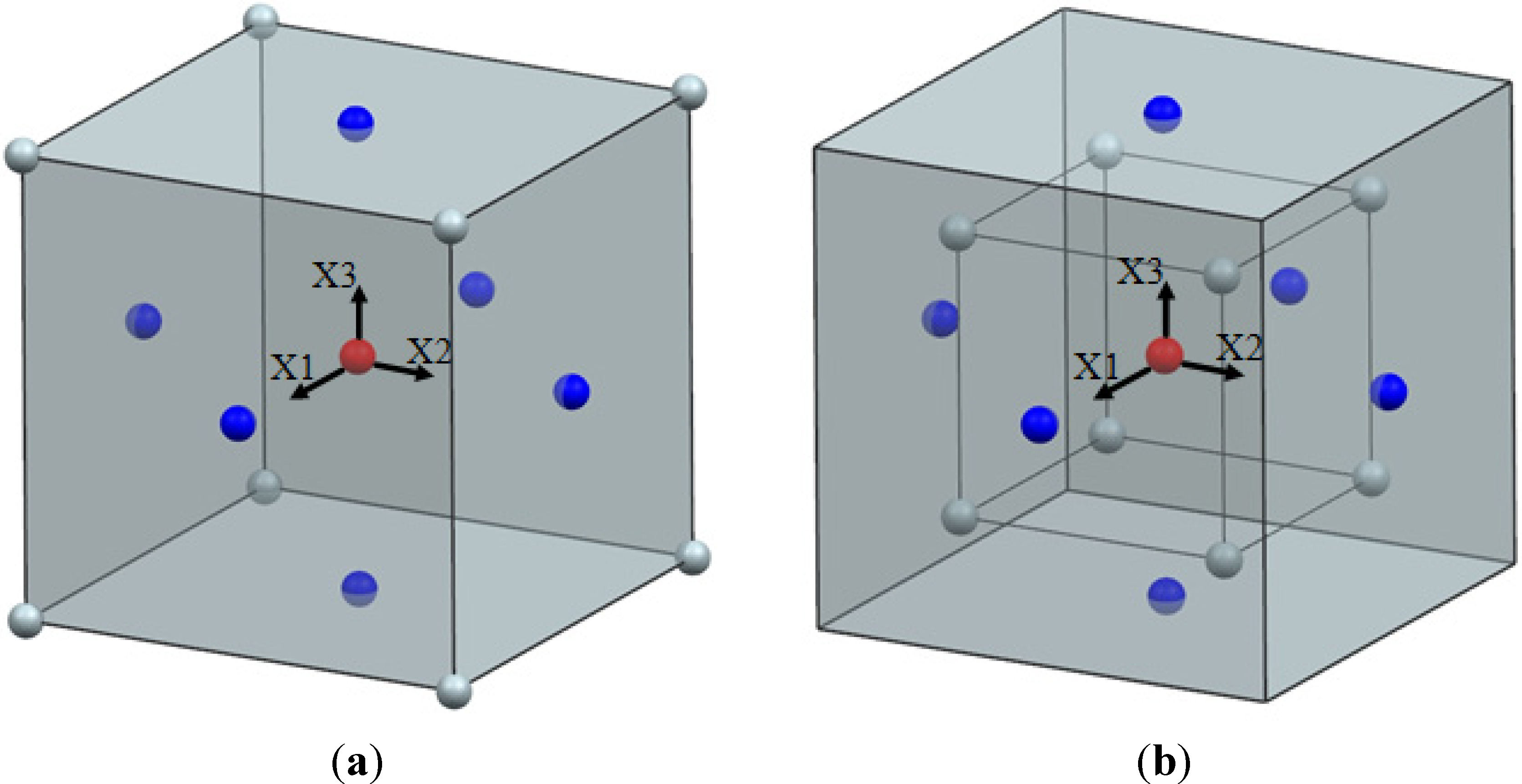
A geometric region restricted by levels −1 and 1 on factor setting is defined as a region of interest to the experimenter. Therefore, based on the positions of factorial and axial points in the design one can distinguish the following main varieties of CCD: circumscribed CCD, face-centered CCD and inscribed CCD. Circumscribed CCD, shown in Figure 3, is the original type of CCD, where axial points are located at distance α, defined by Equation (4), from the center point. In face-centered CCD that is presented in Figure 4, axial points are located at a distance 1 from the center point, i.e., at the face of the design cube, if the design involves three experimental factors. In turn, inscribed CCD is characterized by that axial points are located at factor levels −1 and 1, while factorial points are brought into the interior of the design space and located at distance 1/α from the center point, as illustrated in Figure 4. Geometrically, inscribed CCD reminds of circumscribed CCD. This is because factorial points are set at a distance from the center point so that these distances between the factorial points, the axial points and the center point are in the same proportion as in circumscribed CCD.

Figure 4. Visualization of face-centered CCD (a) and inscribed CCD (b) for three factors: X1, X2 and X3.

Figure 4. Visualization of face-centered CCD (a) and inscribed CCD (b) for three factors: X1, X2 and X3.

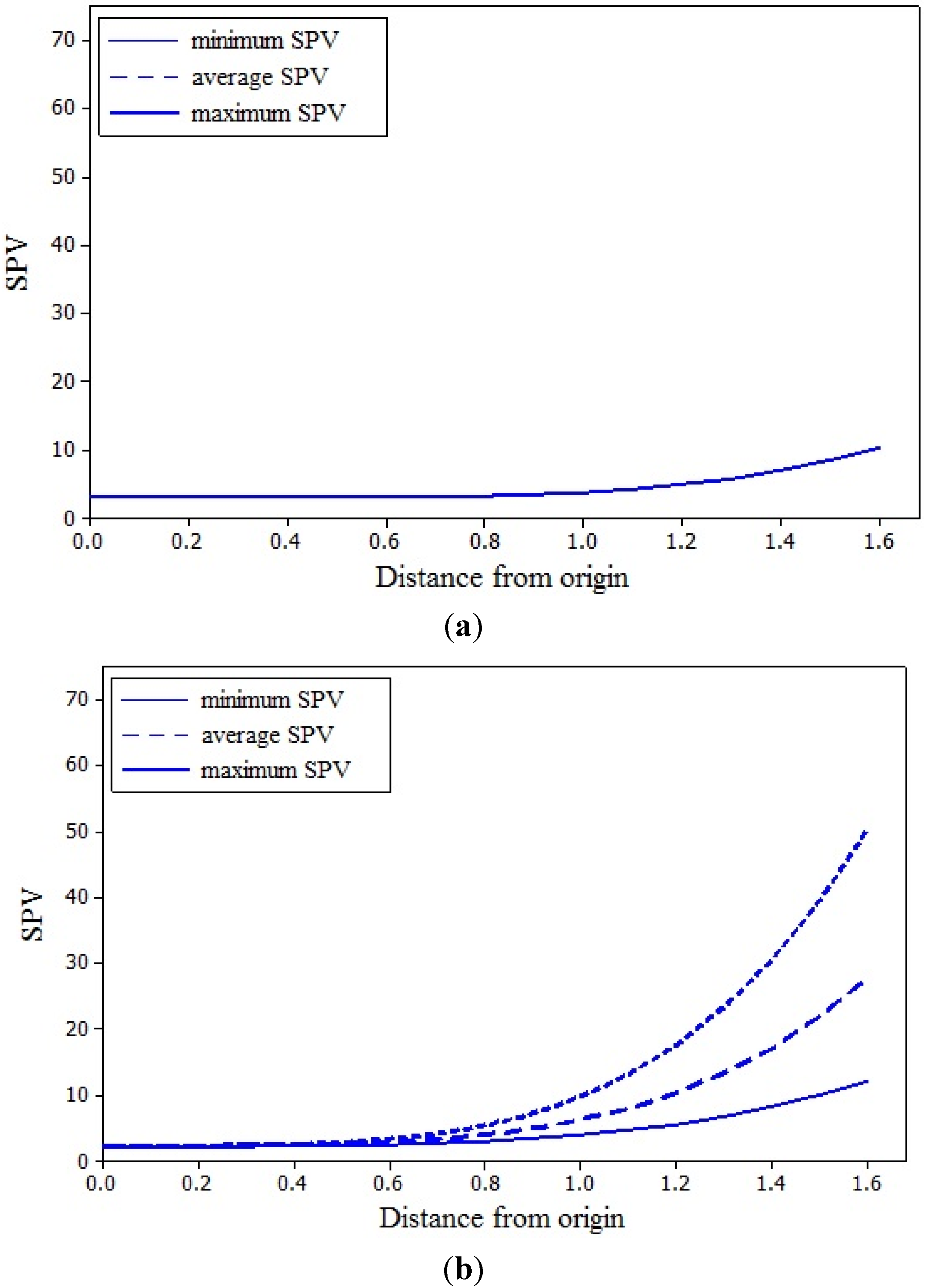
All the varieties of CCD enable the experimenter to study the same region of interest, but they differ in respect of combinations of factor level settings to be tested. However, this affects properties of the prediction variance of a design. Design performance can be evaluated using variance dispersion graph (VDG) [17].

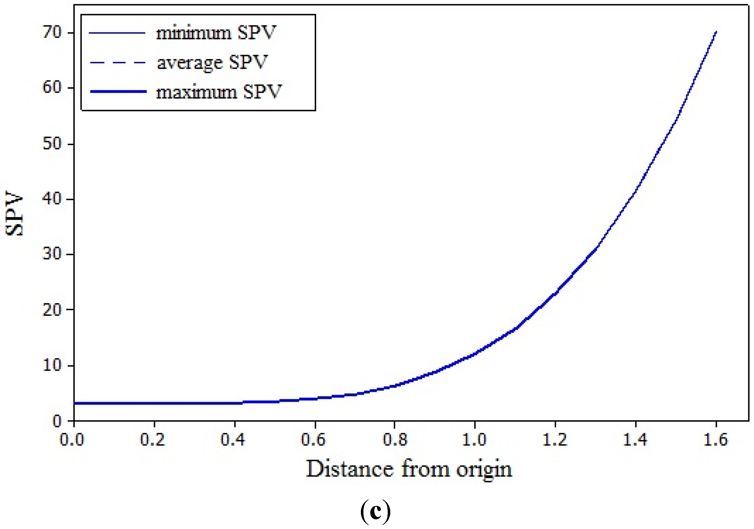
VDG displays the maximum, the minimum and the averaged scaled prediction variance (SPV) against the radius of the spherical space with the center at the center point of the design. SPV can be estimated with the Equation (5):

$$v(x)=\frac{N\cdot Var[y(x)]}{{\mathrm{\sigma }}^2}=\frac{N{\mathrm{\sigma }}^2\cdot x^T{(X^{T}X)}^{-1}x}{{\mathrm{\sigma }}^2}=N\cdot x^T{(X^{T}X)}^{-1}x$$

(5)

where N is the number of points in the experimental design; Var[y(x)] is the variance of a predicted value at a point x; ${\mathrm{\sigma }}^2$ is the variance of the experimental error; X is the design matrix; and x is a vector valued function of the coordinates whose elements correspond to the columns of the design matrix X. According to Equation (5), SPV is independent of the response data and quality of a design can be assessed a priori.

The main varieties of CCD were compared using VDGs, assuming that three factors are tested in the experiment and second-order polynomial model will be developed based on the design. VDGs for the CCDs are shown in Figure 5. SPV for the circumscribed CCD is relatively constant over the distance 1 from the center point of the design. The minimum, the maximum and the averaged SPV are equal at the same distance from the origin and it is evidence that the design is rotatable.

Figure 5. VDGs for: (a) circumscribed CCD; (b) face-centered CCD; (c) inscribed CCD. SPVs plotted in the graphs have been calculated assuming that full quadratic model for 3 factors is tested when running the experiment and each of the designs consists of 20 experimental trials, including 6 center point trials.

Figure 5. VDGs for: (a) circumscribed CCD; (b) face-centered CCD; (c) inscribed CCD. SPVs plotted in the graphs have been calculated assuming that full quadratic model for 3 factors is tested when running the experiment and each of the designs consists of 20 experimental trials, including 6 center point trials.

The face-centered CCD ensures lower SPV near the center point compared to the circumscribed CCD, however, at a certain point of the design SPV increases to a level higher than for circumscribed CCD. Furthermore, the maximum and the minimum SPV at the same distance from the origin are not equal to each other, hence the design is not rotatable. VDG for the inscribed CCD shows the same trend as for the circumscribed CCD, but SPV value is higher. This design is also rotatable, similarly to the circumscribed CCD. Despite the fact inscribed CCD does not require testing factors at as extreme levels as the remaining types of CCD, the penalty for this is seen in the variance, because the further is the distance from the center point, the higher is the variance. It is worth noting that each type of CCD strictly defines design points. Therefore, selection of type of CCD should be made taking into account region of experiment operability. If a design point cannot be tested due to various experiment constraints, the experimenter should reduce factor ranges, what affects the region of interest, or generate face-centered CCD or inscribed CCD.

In practice, no model can be fit perfectly to measured values because of measurement errors or relationships between factors and response that cannot be described by a second-order polynomial. This results in residual values at the design points, i.e., deviations from the measured values. The quality of the model is assessed by the coefficients of determination: R², adjusted R² and predicted R².

R² represents a pure correlation between measured and predicted values and is indicative of the response variation explained by a model [18]. However, every term added to the model equation will improve the model fit to the measured data. Therefore, adjusted R² is used to compare the explanatory power of models, and its value increases only when an added term improves the model more than by chance [18]. Both these coefficients are calculated using data that were themselves used for model development. A model’s predictive capability for new observations is assessed using predicted R². This coefficient is calculated by systematically removing each observation from the data set, estimating the regression equation and determining the model’s capability in predicting the removed observations [19]. Predicted residual sums of squares statistic [20] is used to calculate the value of predicted R².

The statistical significance of the terms of the model defined by Equation (1) can be evaluated using the analysis of variance (ANOVA) [21]. ANOVA is based on partitioning the variation in the data into components. For all the terms of the model equation, values characteristic of a so-called ANOVA table are calculated individually. These values will be important in subsequent discussions and are thus defined here.

The adjusted sum of squares (Adj SS) for a specific term calculates reduction in the residual sum of squares resulting from the inclusion of this term to the model. Adjusted mean squares (Adj MS) are calculated by dividing Adj SS by the number of degrees of freedom (DF) for the respective term.

Variation in the data unexplained by the model is represented by the Residual Error (RE), for which Adj SS is calculated as the residual sum of squares and Adj MS value of the RE is calculated as explained above.

Ratios of the Adj MS for all terms of the model equation and Adj MS of the RE are calculated. Because the ratios of variances follow an F-distribution [16], a statistical F-test [18] is employed to identify statistically significant terms of the model. One can obtain p-values from this test for each term of the model, which are a measure of the probability of obtaining data at least as extreme as the data from the model, assuming that the null hypothesis is true, i.e., in this case, a particular term does not provide an effect on the results from the model [22]. Therefore, the lower the p-values for the analyzed terms, the greater effect these terms have on the response predicted by the model.

Pure error lack-of-fit test [18] is used to assess whether the model is adequate to describe the functional relationships between the experimental factors and the response. The test is based on partitioning the RE sum of squares into two components: lack-of-fit sum of squares, which is associated with variation due to factors other than measurement error, and pure error sum of squares, resulting from random variation caused by measurement error. The ratio of mean squares for lack-of-fit and pure error follows F-statistic, and similar to the aforementioned description, low p-value for lack-of-fit in ANOVA table means that the analyzed model does not fit to the experimental data.

4. Experimental Apparatus and Approach

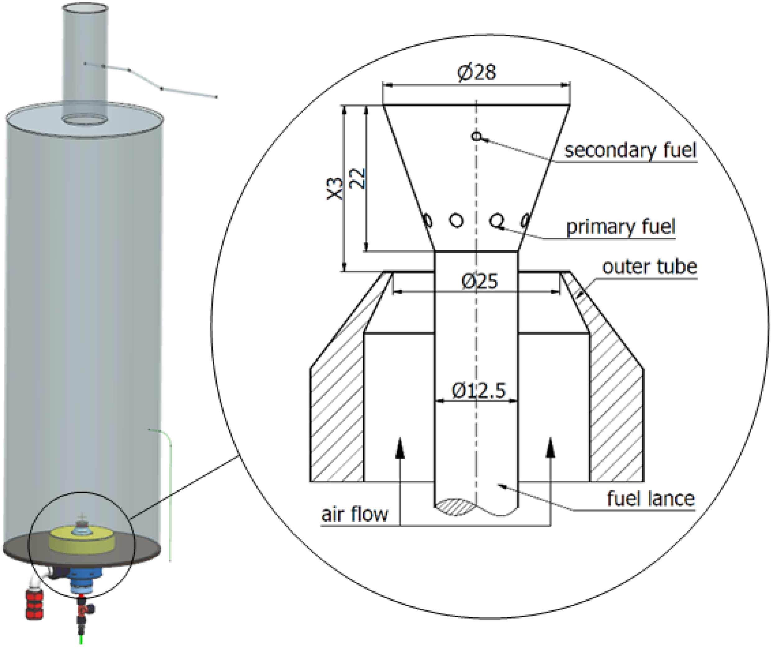
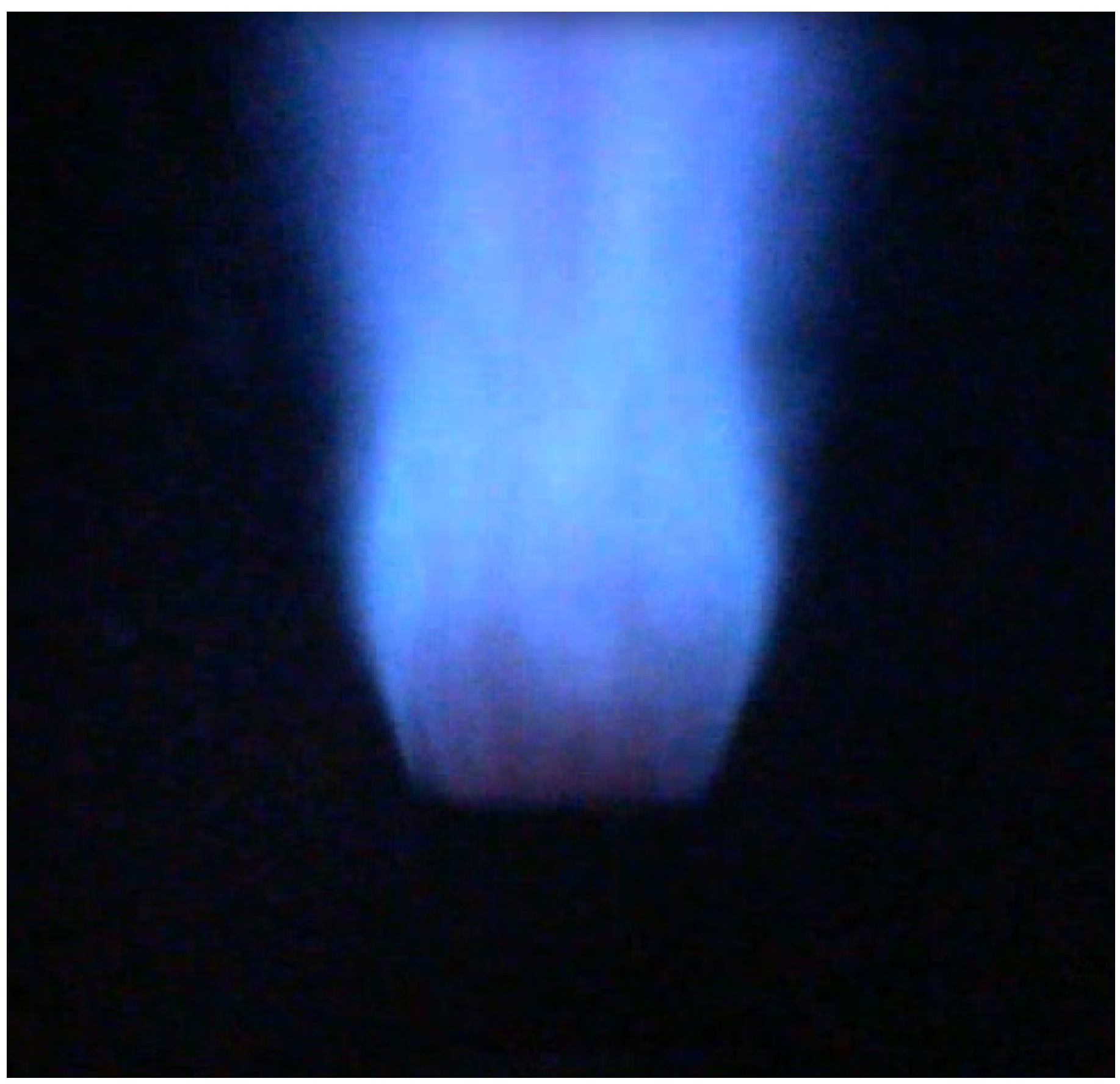
The experimental campaign involved NO_x emission measurements from the PPBB burner, shown in Figure 1, fuelled by pure methane and hydrogen-enriched methane mixtures. All the measurements were conducted at a constant thermal load equal to 25 kW (calculated based on lower heating value, LHV). The fuel mixture was supplied to the burner using two separate fuel supply lines for primary and secondary fuel ports. Mass flow controllers were used to obtain accurate mass flow rates of methane, hydrogen and air to the burner. Maximum measurement error of the mass flow controllers for the investigated burner settings was ±1 nL/min for each fuel supply line and ±10 nL/min for air.

The combustion process took place in a stainless steel combustion chamber at atmospheric pressure. The height of the combustion chamber was 1000 mm with an outer diameter of 360 mm; while the wall thickness was 5 mm. The chamber was cooled only by natural convection and radiation to ambient conditions. The wall temperature was measured on the side of the chamber at a height 300 mm from the bottom to be 390 °C–400 °C. The exhaust gas composition was determined by probing a sample of exhaust gases at the combustion chamber outlet section. The sample was transported through a heated hose to the cooler to avoid uncontrolled water condensation in the gas sampling line and dissolving of nitrogen dioxide (NO₂) in water droplets formed in the hose. NO_x; CO; CO₂ and O₂ were measured with a pre-calibrated Horiba PG-250 gas analyzer. The NO_x concentration in the dry exhaust gas (cooled to 5 °C) was measured by chemiluminescence at a precision of 1 ppmv (part per million by volume); and concentrations of CO₂ and CO were measured using non-dispersive infrared technique. In addition; a Fourier transform infrared gas analyzer was used to measure methane and water concentration in the wet exhaust gas to ensure that all fuel provided to the chamber was burned. The influence of the following four factors on NO_x emissions from the PPBB burner was experimentally investigated:

• hydrogen addition to methane
• amount of excess air
• lance position
• secondary fuel fraction

Levels for the investigated factors were specified as follows: hydrogen content in the fuel was measured by hydrogen mass fraction (X1), excess air was measured using the global air/fuel equivalence ratio (X2), lance position was defined as the distance between the top of the lance and the burner throat (X3) and the amount of secondary fuel was determined as the ratio of the secondary fuel flow rate to the total fuel flow rate (X4).

All the tested factors affect the flow field in the burner and may change the mixing process, flow pattern or flame stability because of complex fluid dynamics. Furthermore, hydrogen addition to methane influences chemical processes occurring in the reaction zone. Interactions between the tested parameters obscure the impact of individual parameters on NO_x emissions from the burner, and the influence of these factors on the emissions cannot be easily described or predicted based on theoretical analyses alone.

Thus, response surface methodology and CCD were employed to identify the significance of each of these factors and develop a second-degree polynomial correlation for NO_x emission prediction. A rotatable CCD was used as the experimental design. Because four factors were studied in the experiment, the number of factorial runs was equal to 2⁴ = 16, and to maintain rotatability in accordance with Equation (4), α was set to 2.

The operating ranges for all the factors were chosen by a series of preliminary measurements to ensure complete fuel combustion and to avoid flame instability, extinction phenomena and combustion chamber acoustic issues at the measurement points. The experimental variables and the levels at which they were tested are shown in Table 1.

Table 1. Tested levels of experimental factors X1, X2, X3 and X4.

Factor	Short Name	Unit	Coded Levels and Corresponding Absolute Levels
			−1	−1/α	0	1/α	1
X1	Hydrogen fraction	%	0	3.75	7.5	11.25	15
X2	Air/fuel equivalence ratio	-	1.05	1.1125	1.175	1.2375	1.3
X3	Lance position	mm	20	21.25	22.5	23.75	25
X4	Secondary fuel fraction	%	0	1.5	3	4.5	6

Table 1. Tested levels of experimental factors X1, X2, X3 and X4.

Factor	Short Name	Unit	Coded Levels and Corresponding Absolute Levels
			−1	−1/α	0	1/α	1
X1	Hydrogen fraction	%	0	3.75	7.5	11.25	15
X2	Air/fuel equivalence ratio	-	1.05	1.1125	1.175	1.2375	1.3
X3	Lance position	mm	20	21.25	22.5	23.75	25
X4	Secondary fuel fraction	%	0	1.5	3	4.5	6

Emission measurement at the center point, i.e., at level zero in coded units for each factor, was replicated four times at various stages of the experiment to obtain an estimate of experimental error. Therefore, the total number of experimental trials, based on the number of design factors k = 4, was equal to N = 2^k + 2k + n_c = 28. Full factorial design represents a possible alternative approach, but it would require a minimum of 3⁴ = 81 experimental trials, while measurement error could not be evaluated and the model would be unnecessarily made far more complicated.

The entire experiment was conducted in random order without replication. The approach enabled the identification of important parameters for NO_x emission reduction and trends in NO_x emissions from the PPBB burner.

5. Results and Discussion

Statistical analysis of the experimental results was performed using the Minitab^® 16 software (Minitab, Inc., State College, PA, USA) [19]. A least squares method was used to derive a mathematical correlation by fitting a response surface to the measured values of NO_x emissions at specific points of the experimental design matrix presented in Table 2. NO_x emissions from the burner have been analyzed for all fuel mixtures investigated, various air/fuel equivalence ratios and burner design parameters.

Table 2. Experimental matrix.

Factor	X1	X2	X3	X4	NOx	CO	NOx	Predicted NOx	Residual
	%	–	mm	%	ppmvd	ppmvd	mg/kWh	mg/kWh	mg/kWh
1	3.75	1.1125	21.25	1.5	17.9	0	35.2	35.2	−0.04
2	3.75	1.2375	21.25	1.5	15.5	5.5	34.3	34.1	0.18
3	11.25	1.1125	21.25	1.5	20.1	0	37.9	37.6	0.35
4	11.25	1.2375	21.25	1.5	17.7	0	37.7	37.7	0.00
5	3.75	1.1125	21.25	4.5	17.9	0	35.3	35.2	0.03
6	3.75	1.2375	21.25	4.5	15.5	7.9	34.2	34.1	0.15
7	11.25	1.1125	21.25	4.5	20.0	0	37.7	37.6	0.13
8	11.25	1.2375	21.25	4.5	18.0	0	38.2	37.7	0.54
9	3.75	1.1125	23.75	1.5	18.5	0	36.3	35.7	0.59
10	3.75	1.2375	23.75	1.5	15.6	4.5	34.6	34.6	0.00
11	11.25	1.1125	23.75	1.5	20.2	0	38.2	38.1	0.13
12	11.25	1.2375	23.75	1.5	17.8	0.1	37.8	38.2	−0.37
13	3.75	1.1125	23.75	4.5	18.0	0	35.4	35.7	−0.29
14	3.75	1.2375	23.75	4.5	15.5	4.7	34.2	34.6	−0.32
15	11.25	1.1125	23.75	4.5	19.9	0	37.5	38.1	−0.53
16	11.25	1.2375	23.75	4.5	17.8	0.1	37.8	38.2	−0.37
17	7.5	1.05	22.5	3	20.2	0	36.4	36.6	−0.17
18	7.5	1.3	22.5	3	15.6	10.0	35.7	35.6	0.12
19	0	1.175	22.5	3	15.4	3.3	32.8	32.9	−0.13
20	15	1.175	22.5	3	19.7	0	38.9	38.8	0.09
21	7.5	1.175	22.5	0	17.8	0	36.4	36.8	−0.44
22	7.5	1.175	22.5	6	17.8	0	36.3	36.8	−0.48
23	7.5	1.175	20	3	17.6	0	36.0	36.3	−0.29
24	7.5	1.175	25	3	18.7	0	38.3	37.3	0.96
25	7.5	1.175	22.5	3	18.0	0	36.8	36.8	−0.02
26	7.5	1.175	22.5	3	18.1	0	37.1	36.8	0.28
27	7.5	1.175	22.5	3	17.7	2.3	36.2	36.8	−0.61
28	7.5	1.175	22.5	3	18.2	0	37.3	36.8	0.51

Table 2. Experimental matrix.

Factor	X1	X2	X3	X4	NOx	CO	NOx	Predicted NOx	Residual
	%	–	mm	%	ppmvd	ppmvd	mg/kWh	mg/kWh	mg/kWh
1	3.75	1.1125	21.25	1.5	17.9	0	35.2	35.2	−0.04
2	3.75	1.2375	21.25	1.5	15.5	5.5	34.3	34.1	0.18
3	11.25	1.1125	21.25	1.5	20.1	0	37.9	37.6	0.35
4	11.25	1.2375	21.25	1.5	17.7	0	37.7	37.7	0.00
5	3.75	1.1125	21.25	4.5	17.9	0	35.3	35.2	0.03
6	3.75	1.2375	21.25	4.5	15.5	7.9	34.2	34.1	0.15
7	11.25	1.1125	21.25	4.5	20.0	0	37.7	37.6	0.13
8	11.25	1.2375	21.25	4.5	18.0	0	38.2	37.7	0.54
9	3.75	1.1125	23.75	1.5	18.5	0	36.3	35.7	0.59
10	3.75	1.2375	23.75	1.5	15.6	4.5	34.6	34.6	0.00
11	11.25	1.1125	23.75	1.5	20.2	0	38.2	38.1	0.13
12	11.25	1.2375	23.75	1.5	17.8	0.1	37.8	38.2	−0.37
13	3.75	1.1125	23.75	4.5	18.0	0	35.4	35.7	−0.29
14	3.75	1.2375	23.75	4.5	15.5	4.7	34.2	34.6	−0.32
15	11.25	1.1125	23.75	4.5	19.9	0	37.5	38.1	−0.53
16	11.25	1.2375	23.75	4.5	17.8	0.1	37.8	38.2	−0.37
17	7.5	1.05	22.5	3	20.2	0	36.4	36.6	−0.17
18	7.5	1.3	22.5	3	15.6	10.0	35.7	35.6	0.12
19	0	1.175	22.5	3	15.4	3.3	32.8	32.9	−0.13
20	15	1.175	22.5	3	19.7	0	38.9	38.8	0.09
21	7.5	1.175	22.5	0	17.8	0	36.4	36.8	−0.44
22	7.5	1.175	22.5	6	17.8	0	36.3	36.8	−0.48
23	7.5	1.175	20	3	17.6	0	36.0	36.3	−0.29
24	7.5	1.175	25	3	18.7	0	38.3	37.3	0.96
25	7.5	1.175	22.5	3	18.0	0	36.8	36.8	−0.02
26	7.5	1.175	22.5	3	18.1	0	37.1	36.8	0.28
27	7.5	1.175	22.5	3	17.7	2.3	36.2	36.8	−0.61
28	7.5	1.175	22.5	3	18.2	0	37.3	36.8	0.51

5.1. Statistical Analysis of the Model

Due to the fact that mixtures of methane and hydrogen were tested during the experiment, it was found that it is useful to express NO_x emissions measured in parts per million by volume on dry basis (ppmvd) as mass of emitted NO_x per unit of heat released during the combustion process. Such definition is independent of O₂ concentration in flue gas, amount of water present in flue gas that is different for methane and hydrogen combustion, and also takes into account various lower heating values of fuels used in the experimental campaign. Therefore, the formula defined by Equation (6) was used to recalculate NO_x emissions to mg/kWh:

$$N{O}_x[\mathrm{mg}/\mathrm{k}\mathrm{W}\mathrm{h}]=\frac{r_{N{O}_x}{V}_{drygas}{\mathrm{\rho }}_{N{O}_x}}{LH{V}_{fuel}}3.6\cdot {10}^6$$

(6)

In Equation (6) r_NOx is measured NO_x emissions expressed in ppmvd; V_{dry gas} is volume of dry flue gas at standard conditions produced from combustion of 1 kg of fuel in Nm³/kg, assuming that the flue gas consists of CO₂, N₂ and O₂; ${\mathrm{\rho }}_{N{O}_x}$ is density of NO₂ at standard conditions equal to 2.05 kg/m³ and LHV_fuel is the lower heating value of fuel mixture used during the burner test in J/kg.

Based on the experimental results of NO_x emissions expressed in mg/kWh and regression analysis for CCD, the full quadratic model is given by Equation (7):

$$\begin{array}{ll}NOx& =-30.011\\ & \hspace{0.17em}-0.418X_1+122.783X_2-0.494X_3+0.400X_4\\ & \hspace{0.17em}-0.017X_1^2-49.402X_2^2+0.053X_3^2-0.052X_4^2\\ & \hspace{0.17em}+1.357X_1{X}_2-0.024X_1{X}_3+0.009X_1{X}_4\\ & \hspace{0.17em}-1.097X_2{X}_3+1.247X_2{X}_4-0.074X_3{X}_4\end{array}$$

(7)

This model takes into account linear effects, quadratic effects and two-way interactions between the studied factors. The empirical correlation represented in Equation (7) must use factors expressed in uncoded units, i.e., actual values of these factors. NO_x emissions obtained using this correlation are given in mg/kWh.

The coefficient of determination R², presented in Table 3, indicates that the model approximates the data at the design points. The predictive power of the developed model for new observations may be 85%, based on the predicted R² value. The calculated p-value for lack-of-fit is greater than 0.05; therefore, there is no statistically significant evidence that the model does not represent the data at a 95% confidence level.

Table 3. Model fitting test results.

Model Parameter	Full Quadratic Model	Enhanced Model
R2	96.63%	94.06%
Adjusted R2	93.01%	92.36%
Predicted R2	84.99%	90.19%
p-value for lack-of-fit	0.75	0.195

Table 3. Model fitting test results.

Model Parameter	Full Quadratic Model	Enhanced Model
R2	96.63%	94.06%
Adjusted R2	93.01%	92.36%
Predicted R2	84.99%	90.19%
p-value for lack-of-fit	0.75	0.195

Based on the results of ANOVA, shown in Table 4, the model was improved by removing terms (one-by-one) with p-values greater than 0.05, considered as statistically insignificant at a 95% confidence level. The removed terms were not taken into account in the regression analysis.

Table 4. ANOVA table for the full quadratic model.

Source of Variation	DF	Adj SS	Adj MS	F-Ratio	p-Value
X1	1	53.2362	53.2362	322.24	<0.001
X2	1	1.5645	1.5645	9.47	0.009
X3	1	1.4741	1.4741	8.92	0.010
X4	1	0.1050	0.1050	0.64	0.440
X1·X1	1	1.4259	1.4259	8.63	0.012
X2·X2	1	0.8937	0.8937	5.41	0.037
X3·X3	1	0.1648	0.1648	1.00	0.336
X4·X4	1	0.3233	0.3233	1.96	0.185
X1·X2	1	1.6182	1.6182	9.80	0.008
X1·X3	1	0.2071	0.2071	1.25	0.283
X1·X4	1	0.0410	0.0410	0.25	0.627
X2·X3	1	0.1176	0.1176	0.71	0.414
X2·X4	1	0.2187	0.2187	1.32	0.271
X3·X4	1	0.3088	0.3088	1.87	0.195
Residual Error	13	2.1477	0.1652
Lack-of-fit	10	1.4444	1.4444	0.62	0.754
Pure error	3	0.7033	0.2344
Total	27

Table 4. ANOVA table for the full quadratic model.

Source of Variation	DF	Adj SS	Adj MS	F-Ratio	p-Value
X1	1	53.2362	53.2362	322.24	<0.001
X2	1	1.5645	1.5645	9.47	0.009
X3	1	1.4741	1.4741	8.92	0.010
X4	1	0.1050	0.1050	0.64	0.440
X1·X1	1	1.4259	1.4259	8.63	0.012
X2·X2	1	0.8937	0.8937	5.41	0.037
X3·X3	1	0.1648	0.1648	1.00	0.336
X4·X4	1	0.3233	0.3233	1.96	0.185
X1·X2	1	1.6182	1.6182	9.80	0.008
X1·X3	1	0.2071	0.2071	1.25	0.283
X1·X4	1	0.0410	0.0410	0.25	0.627
X2·X3	1	0.1176	0.1176	0.71	0.414
X2·X4	1	0.2187	0.2187	1.32	0.271
X3·X4	1	0.3088	0.3088	1.87	0.195
Residual Error	13	2.1477	0.1652
Lack-of-fit	10	1.4444	1.4444	0.62	0.754
Pure error	3	0.7033	0.2344
Total	27

The enhanced model is defined by Equation (8):

$$\begin{array}{ll}NOx& =-20.678\\ & \hspace{0.17em}-0.944X_1+97.837X_2+0.198X_3\\ & \hspace{0.17em}-0.017X_1^2-47.701X_2^2\\ & \hspace{0.17em}+1.357X_1{X}_2\end{array}$$

(8)

This model predicts NO_x emissions in mg/kWh based on three linear effects, two quadratic effects and one two-way interaction. Secondary fuel fraction (X4) has been found to be negligible. Again, the empirical correlation given in Equation (8) must be used with the actual, uncoded factor values.

Although R² and adjusted R², shown in Table 3, decreased compared with those of the full quadratic model given by Equation (7), the enhanced model offers a higher prediction capability of 90.19% for new observations. Simultaneously, with a p-value for lack-of-fit greater than 0.05, it can be assumed that the model adequately represents the experimental results.

A summary of ANOVA applied to the enhanced model is presented in Table 5. The estimated standard deviation of the error in the model is 0.42 mg/kWh. Since all the terms are statistically significant and the model gives reasonable response estimation, it was used to analyze the NO_x emissions from the PPBB burner.

Table 5. ANOVA table for the enhanced model.

Source of Variation	DF	Adj SS	Adj MS	F-Ratio	p-Value
X1	1	53.2362	53.2362	295.01	<0.001
X2	1	1.5645	1.5645	8.67	0.008
X3	1	1.4741	1.4741	8.17	0.009
X1·X1	1	1.4992	1.4992	8.31	0.009
X2·X2	1	0.9259	0.9259	5.13	0.034
X1·X2	1	1.6182	1.6182	8.97	0.007
Residual Error	21	3.7895	0.1805
Lack-of-fit	8	1.9270	0.2409	1.68	0.195
Pure error	13	1.8625	0.1433
Total	27

Table 5. ANOVA table for the enhanced model.

Source of Variation	DF	Adj SS	Adj MS	F-Ratio	p-Value
X1	1	53.2362	53.2362	295.01	<0.001
X2	1	1.5645	1.5645	8.67	0.008
X3	1	1.4741	1.4741	8.17	0.009
X1·X1	1	1.4992	1.4992	8.31	0.009
X2·X2	1	0.9259	0.9259	5.13	0.034
X1·X2	1	1.6182	1.6182	8.97	0.007
Residual Error	21	3.7895	0.1805
Lack-of-fit	8	1.9270	0.2409	1.68	0.195
Pure error	13	1.8625	0.1433
Total	27

5.2. Effects of the Factors

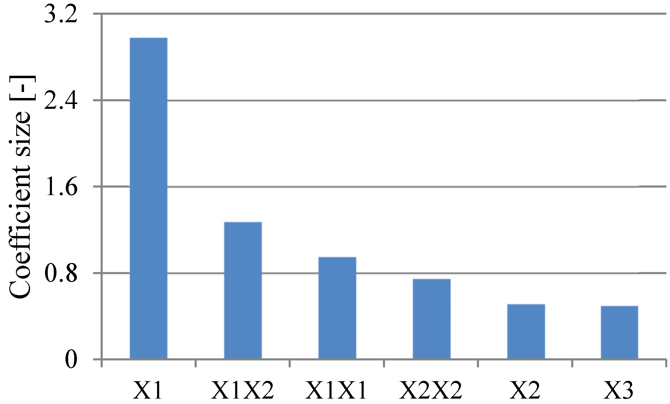
Figure 6 shows the sorted absolute values of the coefficients for each term of the second-degree polynomial based on factors expressed in coded units. Coding of factors removes any pseudo effects due to the use of different measurement scales. Therefore, coefficients in the model equation developed on the basis of coded units are a measure of the magnitude of the response resulting from one unit change in a factor in one specific term, with all other terms held constant. It should be stressed that this interpretation applies over the entire investigated range of factors to linear effects only. Because the model includes an interaction involving two factors (X1 and X2), the effect of a change in one factor associated with the interaction term varies depending on the value chosen for the other factor. In the case of quadratic terms, the response to a change in the value of a factor depends on the value of the factor itself.

Figure 6. Comparison of the absolute values of the coefficients for each term of the enhanced model, which is expressed in coded units.

Figure 6. Comparison of the absolute values of the coefficients for each term of the enhanced model, which is expressed in coded units.

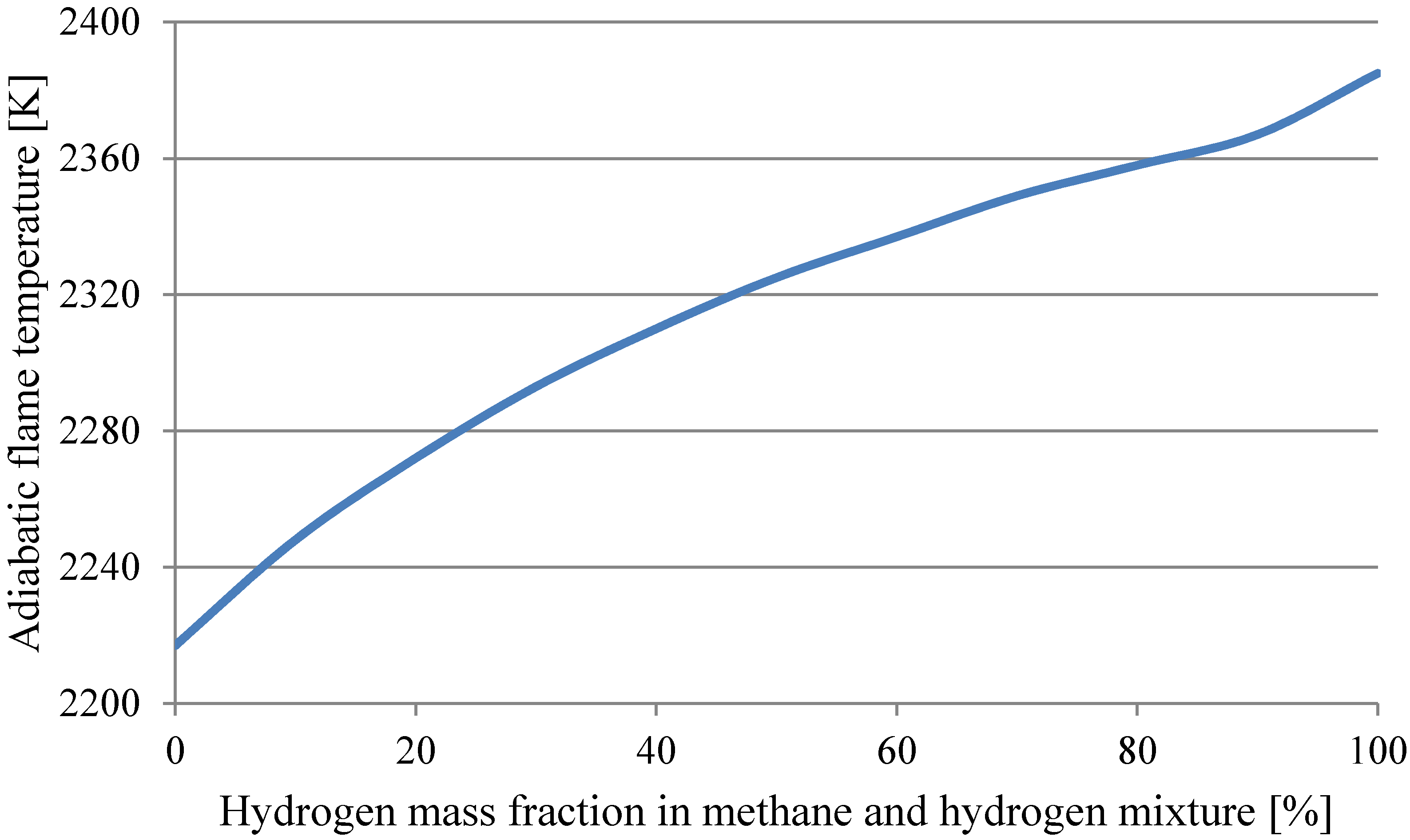
The most significant factor for NO_x emissions is clearly hydrogen fraction in the fuel (X1). The coefficient of the linear term determining fuel composition causes this term to dominate the other terms. Adiabatic flame temperatures, assuming chemical equilibrium of products, for various stoichiometric mixtures of methane and hydrogen and air as oxidizer are presented in Figure 7. Significance of the factor X1for the NO_x emission prediction can as expected be attributed to the increased flame temperature that results from the added hydrogen and thus enhanced thermal NO_x formation.

However, it is worth noting that the above brief explanation does not show the overall picture of the problem and the complexity of NO_x chemistry. When firing hydrocarbon fuels, NO_x are largely formed via thermal or prompt mechanism and, for simplicity, it can be assumed that total NO_x emissions are a combination of these two mechanisms.

Figure 7. Adiabatic flame temperature for various mixtures of methane and hydrogen and air as oxidizer at stoichiometric conditions at pressure equal to 1 atm and temperature of reactants equal to 293 K, calculated assuming chemical equilibrium of products.

Figure 7. Adiabatic flame temperature for various mixtures of methane and hydrogen and air as oxidizer at stoichiometric conditions at pressure equal to 1 atm and temperature of reactants equal to 293 K, calculated assuming chemical equilibrium of products.

The NNH mechanism [23] plays a role in NO_x formation in hydrogen-enriched flames, but it is not discussed here. As it is well-known that hydrogen addition to methane increases flame temperature, it is also known that prompt NO_x formation mechanism requires carbon-containing radicals in the reaction zone. Concentration of these radicals decreases when hydrogen is added to methane and then prompt NO_x formation is inhibited. In the light of the above and despite the fact that NO_x increase is explained here by the higher adiabatic flame temperature of hydrogen-enriched flames, if a low NO_x burner that effectively reduces peak flame temperature is used, the situation when total NO_x emissions from hydrogen combustion are lower than NO_x emissions from pure methane combustion cannot be ruled out [24].

Linear terms related to excess air (X2) and the lance position (X3) are considerably less significant than the hydrogen fraction in the fuel. The effect of the interaction between fuel composition and excess air (X1X2) varies depending on the values of these factors, but for all values of excess air, the interaction affects the response less than hydrogen enrichment of methane. Comparable values for the coefficients of quadratic terms of hydrogen fraction and excess air are evidence that there is a curvature in the response surface describing NO_x emissions. These terms may significantly change the response of the model over the investigated range of factors, depending on the values of the respective factors, but never more than the linear term determining fuel composition. Because the fuel composition is the most important factor, the value of X1 was always taken into account while evaluating the influence of the other experimental variables on NO_x emissions.

5.3. Excess Air Effect

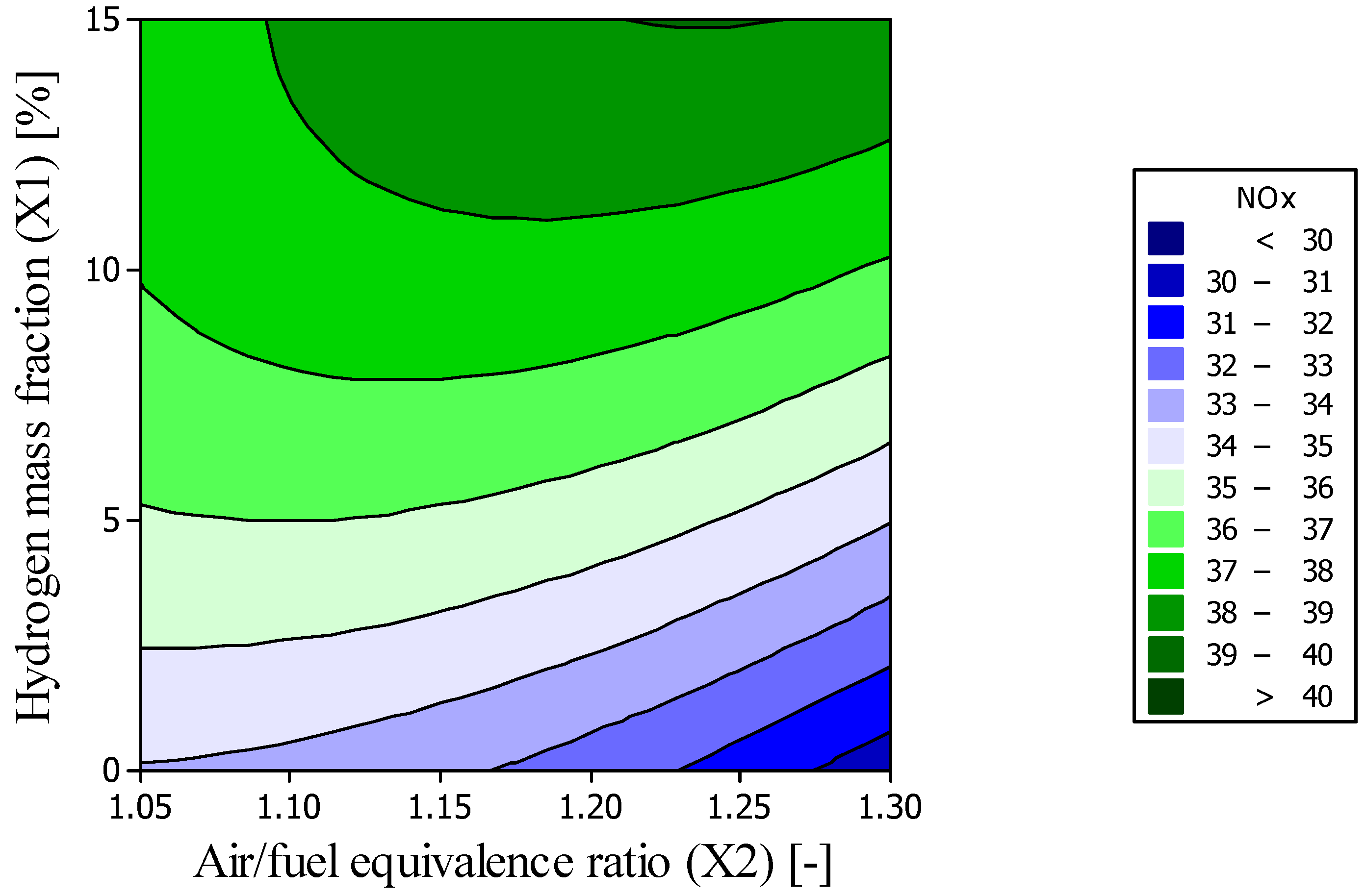
Significant change in NO_x emissions was observed with increasing air flow to the burner in comparison with stoichiometric air consumption in the combustion process. However, this relationship is visible only for pure methane and fuel mixtures containing hydrogen of a few percent mass fraction. As illustrated in Figure 8, with increasing hydrogen content, NO_x emissions approach a state independent of excess air, or even slightly increase with increasing excess air for hydrogen content approaching 15% mass fraction. The lowest NO_x emissions are approximately 30 and 38 mg/kWh for pure methane and hydrogen-rich fuel, respectively. Calculated 95% confidence intervals for these values are between 29.0 and 31.7 mg/kWh, and 37.5 and 40.2 mg/kWh.

Figure 8. NO_x emissions in mg/kWh versus X1 and X2 for the fuel lance positioned at 22.5 mm.

Figure 8. NO_x emissions in mg/kWh versus X1 and X2 for the fuel lance positioned at 22.5 mm.

The relationship shown in Figure 8 can be explained by that additional air plays the role of an inert gas and suppresses NO_x formation via the thermal mechanism. However, for methane enriched with 15% mass fraction hydrogen, this suppressing effect is diminished. Despite the fact that the fuel mixture is partially mixed with air before combustion and the flame is stabilized behind the lance, NO_x emissions are not reduced. It can be assumed that the higher adiabatic flame temperature of hydrogen-enriched methane entails increased thermal NO_x formation, and this mechanism cannot be inhibited by partially premixed air, even at global excess air values approaching 30%. Simultaneously, this effect can be caused by the fact that hydrogen-rich methane-hydrogen-air flame is short and it is stabilized just behind the trailing edge of the lance, while in case of hydrogen-lean methane-hydrogen-air flame or pure methane-air flame, the reaction zone extends over a certain distance further downstream the lance to a better mixed region, for example, due to turbulence. Therefore, in the latter case, higher amount of excess air enables effective reduction of peak flame temperature, what in turn results in lower NO_x emissions.

Note that because the density of hydrogen is approximately eightfold lower than that of methane, hydrogen addition results in increased fuel mixture velocity at the fuel ports. Consequently, air and fuel mixing occurs differently for different fuel mixtures due to different both physical properties such as diffusivity and flow pattern. The amount of excess air provided to the combustion zone behind the lance is probably not linearly dependent on the global excess air value. Therefore, it should be kept in mind when comparing the results that the measured emissions are affected by the different flow fields created by both different fuel composition and excess air. Thus, the extent of NO_x formation may result from either a modified chemical kinetic mechanism, when hydrogen is added, or altered fluid dynamics.

5.4. PPBB Burner Design Parameters Effect

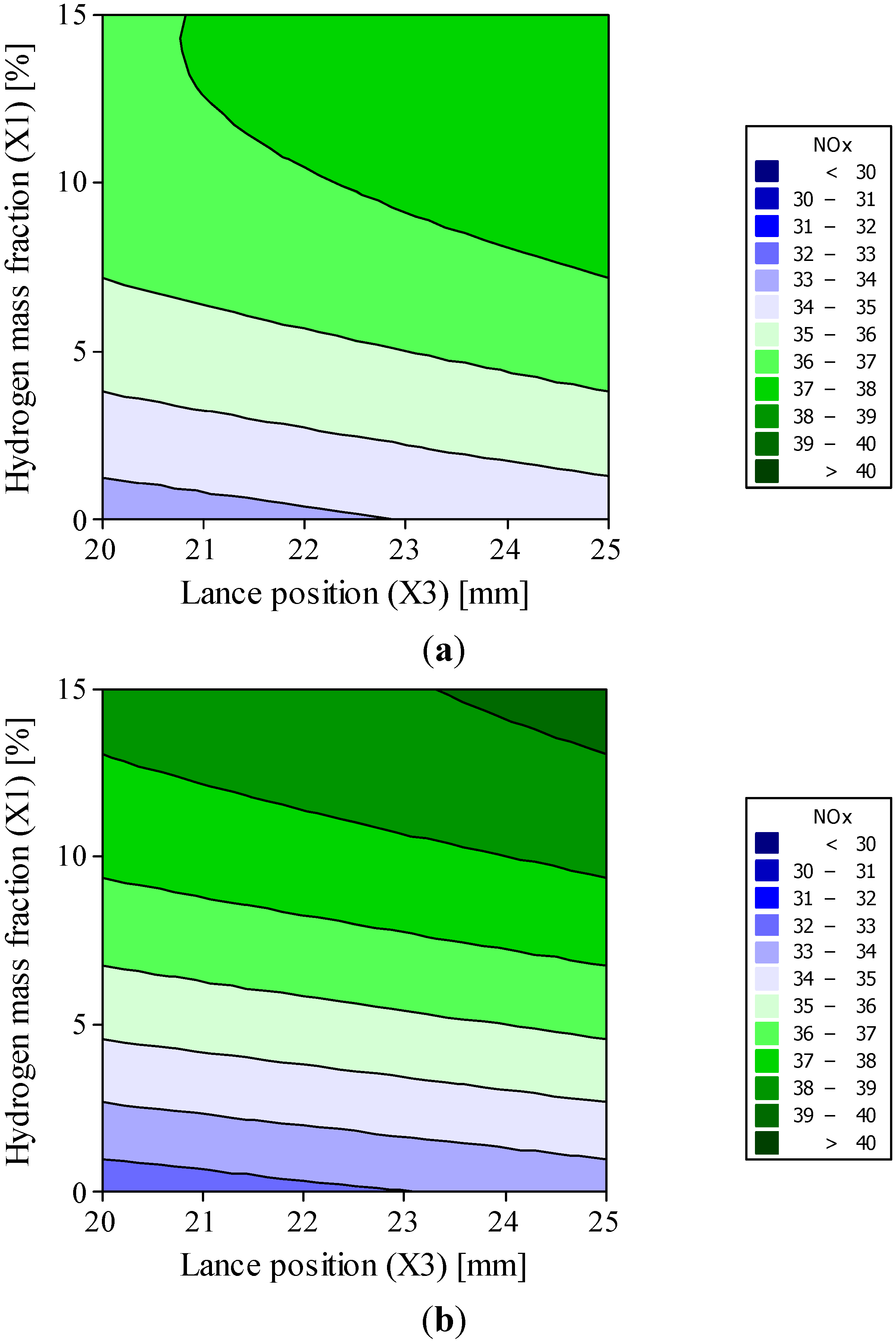
Modifications of the distance between the lance and the burner exit section create variations in air velocity in the air/fuel mixing region. The location of the fuel distribution ports is different for various lance positions. According to Figure 9, for all the investigated fuel compositions, NO_x emissions are reduced with the lance shifted upstream relative to air flow. Minimum NO_x emissions estimated based on 95% confidence interval are between 28.5 mg/kWh and 31.2 mg/kWh, and are observed at a lance position of 20 mm when the burner is fuelled by pure methane. This trend is confirmed for hydrogen-enriched methane as well. However, measurements were conducted with lance positions from 20 to 25 mm because the further shifting of the lance upstream results in incomplete combustion of pure methane. For the investigated settings, primary fuel ports are always located above the top edge of the air outlet, and the lance shape does not substantially affect air velocity at the burner throat, i.e., air outlet section. Therefore, the effect of lance position on NO_x emissions is not strong.

All the terms associated with secondary fuel provided to the burner (X4) were determined to be statistically insignificant over the range of burner settings investigated and have therefore not been included in the enhanced model. The influence of this factor was investigated over rather low mass flow rates ranging from 0% to 6% of total fuel stream. The reason for this was flame extinction, which occurs when a higher amount of secondary fuel is provided to the burner and the burner is fuelled by pure methane. The low settings resulted in the unstable operation of mass flow controllers, and as a result, the influence of this factor may have been underestimated. ANOVA results of the full quadratic model indicated that these terms contributed to the response of the model, with a magnitude lower than the inaccuracy of the model. Quantitatively, the full quadratic model would give approximately the same value for NO_x emissions as the enhanced model. However, the quality of the enhanced model has been improved in that the model facilitates an understanding of the impact of the tested factors on NO_x emissions and has a better predictive capability.

Figure 9. NO_x emissions in mg/kWh versus X1 and X3 for (a) X2 = 1.05; (b) X2 = 1.3.

Figure 9. NO_x emissions in mg/kWh versus X1 and X3 for (a) X2 = 1.05; (b) X2 = 1.3.

5.5. Limitations of the CCD Approach

CCD is perhaps the most popular class of experimental designs, which allow for efficient estimation of second-order response surfaces. Nevertheless, some important limitations have been identified when it comes to application of CCD in the field of combustion.

Second-order polynomial model is unable to describe real behavior of the explanatory variable as a function of the investigated factors, if significant non-linearities or multimodal distribution are present within the tested range of factors. Expert knowledge or additional measurements are necessary in order to ensure that the explanatory variable can be estimated with second-order response surface and higher-order effects do not occur. In contrast to NO_x emissions that can be described by the model developed based on CCD, it was found during preliminary measurements that CCD approach could not be used for CO emission prediction. CO emission trends often exhibit exponential dependence on various factors, e.g., due to so-called CO breakthrough at low amounts of excess air, and thus the predicted values of CO emission do not fit to the experimental data. One possible solution to this problem is to conduct burner tests at a firebox temperature high enough to completely oxidize CO formed in the reaction zone, and focus only on NO_x emissions, as it was done in the experiment described above. Reasonableness of this approach is, however, conditioned by the target application of the tested burner, i.e., whether it will be used in high-temperature furnaces or low-temperature furnaces [25]. It is worth noting that NO_x emissions are dependent on a firebox temperature [26], but as soon as combustion process is complete, means all CO is reburned to CO₂, optimal burner design parameters determined at a certain firebox temperature are still optimal in terms of emissions at a higher firebox temperature.

Another important limitation of the CCD is the fact that this approach requires symmetrical design space. In other words minimum and maximum values of tested factors must be equidistant from the respective values of these factors at a center point. It may be a significant disadvantage when CCD is used for burner development, because conducting measurements at certain points of the design may not be possible due to operational reasons. At certain combinations of factors tested within the design, burner operation may not be stable or even possible due to difficulties such as: unacceptably high CO emission, flame instability or extinction, chamber acoustic issues, and flame stabilization at surfaces, which are not designed for this purpose. These issues naturally affect region of experiment operability and they may cause that it can be highly asymmetrical. An easy way to deal with these difficulties is to resign from testing the most limiting factor or narrow ranges of the factors tested in an experiment. However, one may be also interested in NO_x emissions beyond the symmetrical design space of the reduced CCD, which is fitted into a wider region of operability. If it is the case, an alternative approach to experimental design is D-optimal or I-optimal design. The former aims to minimize the variance of the factor-effect estimates, while the latter minimizes the average variance of prediction over the region of experimentation and it makes I-optimal design more appropriate for prediction than D-optimal design [27]. These methods offer a great deal of flexibility to reach a viable compromise between number of experimental trials, design choices, constraints, and usable results. On the other hand, the disadvantage of the optimal designs is that they are model-dependent. It means that they require knowledge about form of a model, i.e., knowledge of terms of the second-order polynomial which should be used for a proper description of the relationship between the response and the factors. This information is necessary to generate optimal design and the form of the model must be specified by the experimenter a priori. Testing of all the unique combinations of factors overcomes all the aforementioned difficulties, but reasonableness of this approach is, of course, dependent on its intended purpose and available resources.

6. Conclusions

NO_x emissions from a laboratory-scale PPBB burner were investigated using a CCD of the experiment. Experimental measurements were conducted at a constant thermal load equal to 25 kW (calculated based on LHV). The influence of hydrogen enrichment of methane, excess air and burner design parameters on NO_x emissions was analyzed. The developed model allowed for an evaluation of linear and quadratic effects of analyzed factors, as well as significant interactions between these factors. The significance of the model terms was assessed by ANOVA. The values predicted by the second-order polynomial model are well-aligned with the measured NO_x emissions. Limitations of the used approach to experimental design have been identified and discussed.

Based on the developed model, it was found that addition of hydrogen to methane is accompanied by an increase of NO_x emissions. While this effect is very strong and cannot be avoided, it can be reduced by properly selecting burner operation settings. Increase in excess air results in significant NO_x emissions reduction, but only when the burner is fuelled by pure methane or fuel mixtures containing small amounts of hydrogen. However, NO_x formation is largely insensitive to changes in global excess air when the burner is fuelled by methane enriched with about 15% mass fraction hydrogen. This can be attributed to the location of hydrogen-enriched reaction zone close to the lance in a poorly mixed region and a higher adiabatic flame temperature, resulting in an enhanced thermal NO_x formation mechanism. A proper fuel lance position enables slight reduction of NO_x emissions. Secondary fuel fraction was found to have no significant effect on NO_x emissions over the investigated range of burner operation settings.

The developed correlation demonstrates that response surface methodology combined with a CCD of the experiment can be used as an effective method for investigating the influence of various factors on NO_x emissions and finding optimal burner operation settings, if such exist. The technique is also useful in a context where numerous factors affecting the results are involved, and factors warranting deeper insight can be highlighted.