Application of Satellite-Based Spectrally-Resolved Solar Radiation Data to PV Performance Studies

Abstract

In recent years, satellite-based solar radiation data resolved in spectral bands have become available. This has for the first time made it possible to produce maps of the geographical variation in the solar spectrum. It also makes it possible to estimate the influence of these variations on the performance of photovoltaic (PV) modules. Here, we present a study showing the magnitude of the spectral influence on PV performance over Europe and Africa. The method has been validated using measurements of a CdTe module in Ispra, Italy, showing that the method predicts the spectral influence to within ±2% on a monthly basis and 0.1% over a 19-month period. Application of the method to measured spectral responses of crystalline silicon, CdTe and single-junction amorphous silicon (a-Si) modules shows that the spectral effect is smallest over desert areas for all module types, higher in temperate Europe and highest in tropical Africa, where CdTe modules would be expected to yield +6% and single- junction a-Si modules up to +10% more energy due to spectral effects. In contrast, the effect for crystalline silicon modules is less than ±1% in nearly all of Africa and Southern Europe, rising to +1% or +2% in Northern Europe.

1. Introduction

It is well known that the energy conversion efficiency of photovoltaic (PV) cells depends on the wavelength of the incoming light [1–4]. This so-called spectral response of the cell depends on the PV technology used. Since the spectrum of sunlight varies over time, the power output of PV cells and modules will depend not only on the total in-plane irradiance, but also on the instantaneous spectrum of the sunlight. As a result, the different spectral responses of PV technologies will cause PV modules to have different instantaneous power output, even if they have the same nominal power [5–8]. If the solar spectrum differs significantly between geographical locations, this may lead to a difference in the overall energy output from PV installations. Knowing the effect of the spectral variations at any point would therefore be useful for PV system planners and investors in order to choose the PV modules best suited for a given location.

Measuring the spectrum of sunlight is much more difficult and expensive than measuring the broadband radiation using pyranometers. Mainly for this reason, the number of sites where the spectrum has been measured consistently is relatively small. This, in turn, means that assessing the influence of the spectral variations on PV energy output at a given site is very difficult.

Even when the task of collecting spectrally resolved data is discounted, the analysis of the collected information still poses difficulties. Adequately characterizing a solar spectrum typically involves obtaining measurements at a resolution of 2 nm over the wavelength range of 300–1700 nm. Instead of one data point per measurement, as would be obtained with a pyranometer, several hundred data points are acquired. Since the variation of any one of these data points alone is not enough to influence the measurable output of a photovoltaic system, it becomes necessary to find some average value or values that will indicate a general shift in the distribution of light over the spectrum.

One such metric that has gained popularity within the photovoltaic community is the “average photon energy” (APE) proposed by Jardine et al. in [9]. Similar to an average photon wavelength [10], it represents the average energy of all of the photons impinging upon a target surface and is typically expressed in units of electron-volts. Unlike a spectral mismatch value or the “Z parameter” [11], it is a technology-independent parameter that describes only the spectral quality of solar irradiation. Some authors have argued that an APE value will describe a single spectral distribution of irradiance to within a level of certainty sufficient for PV analyses [12]. Other researchers have presented evidence that this is not the case [8]. With the present results, we hope to add to this discussion.

Recently, methods have been developed to estimate the spectral content of sunlight using data from geostationary satellites [13,14]. These data have uniform coverage over large geographical areas; for instance, the Meteosat class of satellites cover Europe, Africa and nearly all of Asia. The spatial resolution is generally a few kilometers. The satellite data record covers up to 30 years in some regions, and the time resolution is typically hourly or better.

It should therefore be possible to use such satellite retrieved data together with information about the spectral response of PV modules in order to estimate the overall influence of spectral variations on the PV energy output. However, this will of course only be possible if the spectrally-resolved radiation data are sufficiently accurate, so as to give meaningful estimates of the spectral variations in the PV output.

The aim of this paper is to investigate the possibility of using the satellite-based spectral irradiance data to estimate the effect of spectral variations on PV energy output and to quantify the magnitude of this effect over large geographical areas. The structure of the paper is as follows: Section 2 briefly describes the satellite-based spectral irradiance data. We then present the mathematical models used to estimate the PV performance in Section 3. Section 4 contains the validation of the spectrally-resolved irradiance data, both for global horizontal and direct normal irradiance. This section also describes the validation of the model for calculating the influence of spectral variations, using outdoor measured PV performance data. The application of the models to calculate the spectral effect over large geographical regions is then given in Section 5.

2. Satellite-Based Estimates of Spectrally-Resolved Solar Radiation Data

2.1. Retrieval of Spectrally-Resolved Solar Radiation Data from Satellite Images

The SPECMAGIC algorithm calculates spectrally-resolved solar irradiance using the effective cloud albedo [15] retrieved from geostationary meteorological satellites combined with data on the atmospheric content of aerosols, water vapor and ozone. Aerosol information is taken from the Monitoring Atmospheric Composition & Climate (MACC) project. The MACC aerosol data result from a data assimilation system for global reactive gases, aerosols and greenhouse gases. It consists of a forward model for aerosol composition and dynamics [16] and the data assimilation procedure described in detail in [17]. The data are generated by the European Centre for Medium Range Weather Forecast on a Gaussian T159, which is transformed to a 0.5 × 0.5° regular latitude longitude grid. The water vapor profile results from the reanalysis of the European Centre for Medium-Range Weather Forecasts [18,19]. Monthly values have been used at a 0.25 × 0.25° grid. For ozone, climatological standard profiles provided within the radiative transfer model “libRadtran” are used [20].

The algorithm, which is described in Müller et al. [13], calculates both global horizontal (GHI) and direct normal irradiance (DNI) in 30 spectral bands in the range from 300 nm–4,600 nm. The spatial resolution of the radiation data is three arc-minutes. Irradiance has been calculated using the Meteosat satellites covering Europe, Africa and nearly all of Asia [21]. The spectral bands used in the algorithm are identical to the 32 bands used by Kato et al. [22], except for the first two bands in the ultraviolet. The lower and upper limits of the 32 Kato bands are provided in

Table A1. Lower and upper limits in nm of the 32 Kato bands.

Kato Band	Lower Limit (nm)	Upper Limit (nm)
1	240.1	272.5
2	272.5	283.4
3	283.4	306.8
4	306.8	327.8
5	327.8	362.5
6	362.5	407.5
7	407.5	452.0
8	452.0	517.7
9	517.7	540.0
10	540.0	549.5
11	549.5	566.6
12	566.6	605.0
13	605.0	625.0
14	625.0	666.7
15	666.7	684.2
16	684.2	704.4
17	704.4	742.6
18	742.6	791.5
19	791.5	844.5
20	844.5	889.0
21	889.0	974.9
22	974.9	1,045.7
23	1,045.7	1,194.2
24	1,194.2	1,515.9
25	1,515.9	1,613.5
26	1,613.5	1,964.8
27	1,964.8	2,153.5
28	2,153.5	2,275.2
29	2,275.2	3,001.9
30	3,001.9	3,635.4
31	3,635.4	3,991.0
32	3,991.0	4,605.7

of the Appendix.

The uncertainty of the retrieval algorithm is typically below 1%–2%, which has been estimated by comparison with radiative transfer model based methods; please see [13] for further details. This uncertainty is significantly lower than the experimental error of about 5% of spectro-radiometric measurements [23], but does not include the errors induced by the used atmospheric input, which is likely the main error source for the estimation of solar surface irradiance. The accuracy of the retrieved spectrally-resolved irradiance depends on the specific sites and spectral region and is further discussed in Section 4.1 of this manuscript, as well as in [13]. Typically, the error is close to the measurement error of the ground-based spectro-radiometric measurements.

2.2. Calculation of Inclined-Plane Radiation

Given the global horizontal and direct normal (or horizontal) irradiance, the direct irradiance can be calculated on any arbitrary plane [24]. There exists a number of models for estimating the diffuse irradiance on an inclined plane [25,26]. In this work, we use a modified version of the model developed by Muneer [25]. The modification was necessary because the model uses the clearness index k_c (Equation (1)) as an input parameter:

$$k_c=\frac{G}{G_{\mathrm{e}xt}}$$

(1)

where G and G_ext are, respectively, the horizontal irradiance at the Earth’s surface and at the top of the atmosphere. When using this model for spectrally-resolved irradiance, it becomes necessary to substitute both G and G_ext by the corresponding irradiances in each spectral band in order to calculate k_c for that band.

3. Models and Data for PV Performance Studies

The power output of a PV module or array depends on a number of different environmental influences. In this study, we will consider some of these in order to estimate how the output power varies with:

• Increased reflectivity at a shallow angle of incidence;
• The effect of the spectrum of the sunlight;
• The effects of module temperature and irradiance.

Some other effects will not be considered here, such as aging of the modules, local shadows or deposition of dust, dirt or snow on the modules. For some of these effects, the geospatial variation is poorly known, while other effects, such as shadowing, are likely to be extremely local and not suited for studies over large geographical regions.

3.1. Influence of Angle of Incidence on the Transmitted Irradiance

When light strikes the surface of a PV module at a sharp angle of incidence (light rays are nearly parallel to the module surface), there is increased reflection of the light, and the output is correspondingly lower. In the calculations described here, we use the model of Martin and Ruiz [27] to account for this effect. This model assumes that the angular dependence of reflectivity is the same for all wavelengths.

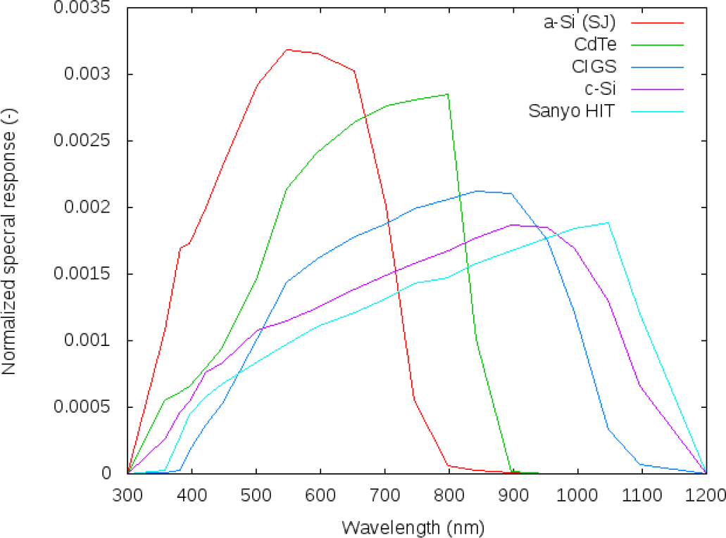
3.2. Effects of Changes in the Light Spectrum

The efficiency with which the energy of the photons in sunlight is converted into electrical energy in the PV cell depends on the photons’ wavelength. Some photons have insufficient energy to excite an electron in the PV material, while others have excess energy that cannot be transferred to the electrons. The sensitivity of a given PV cell to different light wavelength is called the spectral response or spectral response curve, denoted S_r(λ). The spectral response is a function of wavelength and at each wavelength is proportional to the conversion efficiency of the cell/module when illuminated with monochromatic light of that wavelength. This is not the case for multijunction PV cells, so this description does not apply to these PV technologies.

Some spectral response curves are shown in Figure 1. These spectral response curves were measured at the ESTI Laboratory of the European Commission Joint Research Centre. The methods used to measure the spectral response curves are described in [4,28].

The short-circuit current I_sc is very nearly proportional to the number of electrons that are excited in the PV material per second. As shown in Equation (2), for a given wavelength λ, the contribution to I_sc is proportional to the spectral response multiplied by the intensity of the light at that wavelength. I_sc can then be found by integrating this over the wavelength range where S_r(λ) > 0:

$$I_{sc}=k{\displaystyle \int S_r(\lambda )R(\lambda )d\lambda }$$

(2)

Here, R(λ) is the spectral light intensity and k a proportionality constant specific to the given cell/module and the measured spectral response curve.

The power of a PV module is not proportional to I_sc, since it also depends on the module voltage. However, for small changes in the power, the variation in the voltage is small, and the power will be approximately proportional to I_sc:

$$\mathrm{\Delta }P\propto \mathrm{\Delta }{I}_{sc}$$

This would be the case when the spectrum changes, but the total irradiance stays the same.

Following [6,8], the effect of spectral changes can then be estimated as the spectral mismatch, MM (Equation (3)):

$$MM=\frac{{\displaystyle \int S_r(\lambda )R(\lambda )d\lambda }}{{\displaystyle \int S_r(\lambda )R_{STC}(\lambda )d\lambda }}\cdot \frac{G_{STC}}{G_{POA}}=\frac{I_{sc}}{I_{sc,STC}}$$

(3)

Here, R_STC is the spectrum defined in the standard test conditions (STC), G_STC is the total broadband irradiance of the STC spectrum, while G_POA is the broadband irradiance in the plane of array (found by integrating R(λ)). I_sc,STC is the short-circuit current under the STC spectrum and irradiance.

The mismatch factor MM can now be used to define an effective irradiance, G_eff, from the received in-plane of array irradiance G_POA (Equation (4)), which can be used to estimate the output power of the PV module.

$$G_{eff}=MM\cdot G_{POA}$$

(4)

3.3. Model for PV Performance

It is well known that the power output of a PV module depends on the received irradiance in a nonlinear way and also on the temperature of the module. The importance of these effects varies between PV technologies.

There exist a number of different models to account for these effects in the literature [29–32]. The model used in this work is described in Huld et al. [32]. According to this model, the instantaneous power can be described, as shown in Equation (5), as a function of the effective in-plane of array irradiance G_eff and the module’s temperature T_mod:

$$P(G_{eff},T_{\mathrm{mod}})=P_{\mathrm{nom}}\frac{G_{eff}}{G_{STC}}{\mathrm{PR}}_m(G_{eff}^{\prime },T^{\prime })$$

(5)

where G_STC =1,000 W/m² is the STC irradiance and $G_{eff}^{\prime }$ and T′ are irradiance and temperature values normalized to STC values according to Equation (6):

$$G_{eff}^{\prime }\equiv G_{eff}/G_{STC},T^{\prime }\equiv T_{\mathrm{mod}}-25°\mathrm{C}$$

(6)

PR_m is the module performance ratio; its dependence on $G_{POA}^{\prime }$ and T′ is shown in Equation (7):

$${\mathrm{PR}}_m=1+k_1\ln (G_{eff}^{\prime })+k_2{(\ln (G_{eff}^{\prime }))}^2+T^{\prime }\left[k_3+k_4\ln (G_{eff}^{\prime })+k_5{(\ln (G_{ef}^{\prime }))}^2\right]+k_6{T^{\prime }}^2$$

(7)

The coefficients k₁ to k₆ must be found by fitting the model to experimental data measured on the module or module type of interest.

PR_m depends on the instantaneous irradiance and module temperature. Under steady-state (or slowly changing) conditions, the T_mod can be estimated from the ambient (or air) temperature T_amb, wind speed W and the in-plane of array irradiance in the following way (Equation (8)) [33,34]:

$$T_{\mathrm{mod}}=T_{\mathrm{amb}}+\frac{G_{POA}}{u_0+u_{1}W}$$

(8)

The coefficients u₀ and u₁ describe how much the PV module is heated by the solar radiation and cooled by the wind. They depend on the way the PV module is mounted (free-standing rack, ventilated or unventilated roof mounting, etc.) and also slightly on the module type.

In the applications of this model, in the following, we have used values for u₀ and u₁ taken from Köhl et al. [34].

3.4. Sources of PV Module Data

The models for PV power estimation given in Sections 3.1–3.3 contain coefficients that must be determined from measurements performed on the PV modules. For the angle-of-incidence (AOI) effect, we have used coefficients taken from the literature [27].

Data for the module temperature model have been taken from [34]. The coefficients for a free-standing rack are given in

Table 1. Values of coefficients u₀ and u₁ used in Equation (8) for different photovoltaic (PV) technologies.

Module Type	u0 (W/(°C.m2))	u1 (W.s/(°C.m3))
c-Si	26.9	6.20
CdTe	23.4	5.44
a-Si	25.7	6.29

.

For the PV power model in Equation (7), coefficients for typical crystalline silicon modules can be found in [32]. The coefficients for CdTe and a-Si are based on measurements performed by the JRC ESTI laboratory and fitted using the methods described in [32].

4. Validation

Some validation results for the SPECMAGIC spectrally-resolved irradiance data have been reported in [13] for two sites in Europe, for global spectral irradiance on an inclined plane. Here, we will add results for one site for global horizontal spectral irradiance and one site for spectral direct normal irradiance (DNI). The DNI spectrum is important in this context, because it is needed to calculate the inclined-plane spectral irradiance.

The validation of the spectrally-resolved irradiance values derived from the SPECMAGIC algorithm is performed using measurements of global horizontal and direct (beam) normal spectral irradiance registered at two different locations, Ispra (Italy) and Nicosia (Cyprus), respectively. A detailed description of the two measured databases, including the procedure followed to register and record the spectral irradiance measurements, the instruments used, the wavelength range covered and the temporal resolution of the recordings, can be found in [35] for the global irradiance database and in [36] for the direct irradiance database.

The spectroradiometer system installed in Cyprus has been calibrated in situ by performing a calibration transfer from a reference set of spectroradiometers. This reference set was, in turn, calibrated at the European Solar Test Installation laboratories against an FEL (filament type) standard lamp calibrated at the National Physics Laboratory (NPL). The average uncertainty budget for the calibration of the outdoor spectroradiometers has been estimated using the known calibration drift of these devices, the noise levels present, the sensor linearity and the uncertainties involved in the outdoor transfer. This has resulted in an estimated expanded uncertainty of calibration of ±5.4%. A full breakdown of this estimate has been described in [36]. The measurement uncertainty is more difficult to estimate due to the large number of variables that can affect each measurement, but accounting for the same uncertainty components again results in a first estimate of expanded uncertainty of ±6.69%.

However, a brief description of the measured databases and the period of time used for this particular analysis is presented in

Table 2. Description of the measured spectral irradiance datasets used. GHI, global horizontal; DNI, direct normal irradiance.

Location	Ispra (Italy) (45.81° N, 8.62° E)	Nicosia (Cyprus) (35.15° N, 33.42° E)
Variable (W/m2/nm)	Spectral GHI	Spectral DNI
Period of time analyzed	2009: January–December 2010: January–June	2013: August–September
Wavelength range (nm)	400–2,500	300–1,700
Wavelength step (nm)	2	2
Temporal resolution (minutes)	30	5
Initial number of measurements	10,411	7,091

.

While the measured data contain the spectral irradiance registered every few nm, the output of the satellite algorithm is the spectral irradiance already integrated into 30 bands (“Kato bands”) of different wavelength widths in the range from 300 nm–4600 nm. Another difference between the measured databases and the estimated one is the time frequency of the data. While measurements are performed every few minutes, the frequency of the estimated values depends on the availability of the satellite images. For this validation, there are two estimated values available per hour for Nicosia and one per hour for Ispra. These differences between the measured and estimated data make it necessary to perform some modifications to the original measured values before comparing measured and estimated irradiance values in the validation. The procedure applied goes as follows:

• For every satellite retrieved time point, the closest measurement in time to the moment when the satellite image was taken is selected from the measurement time series. Due to the frequency of the measured data, a 5-min window centered at the moment of the satellite data was applied for the Cyprus database and a 20-min window was used for the Ispra database.
• The measured spectral irradiance values are integrated into bands according to the limits of the Kato bands available in the estimated database. However, due to the wavelength range of the equipment used to measure the spectral irradiance, not all of the 30 bands available in the estimated database can be considered.
• It was decided to remove all of the moments when the Sun’s elevation angle is below 5°.

Once the measured data have been treated according to the previously described procedure, measured and estimated irradiance values in every Kato band can be compared in order to validate the performance of the SPECMAGIC algorithm. The output of SPECMAGIC consist of irradiance in each of the Kato bands. However, since the widths of these bands vary strongly, the derived irradiance values are not very informative. Instead, we will show the results of the validation with these two sets of values:

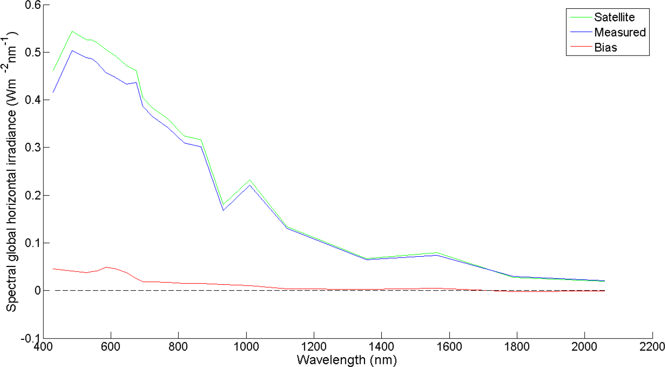
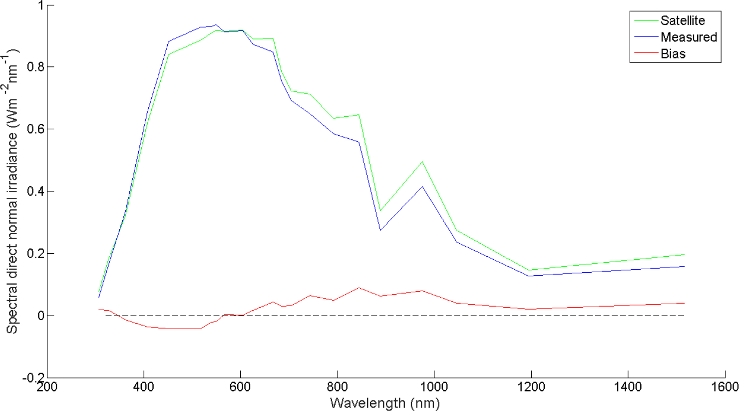
• spectral irradiance in every band calculated by dividing the irradiance values in each Kato band by the width of the band in nm, R_λ (W/m²/nm);
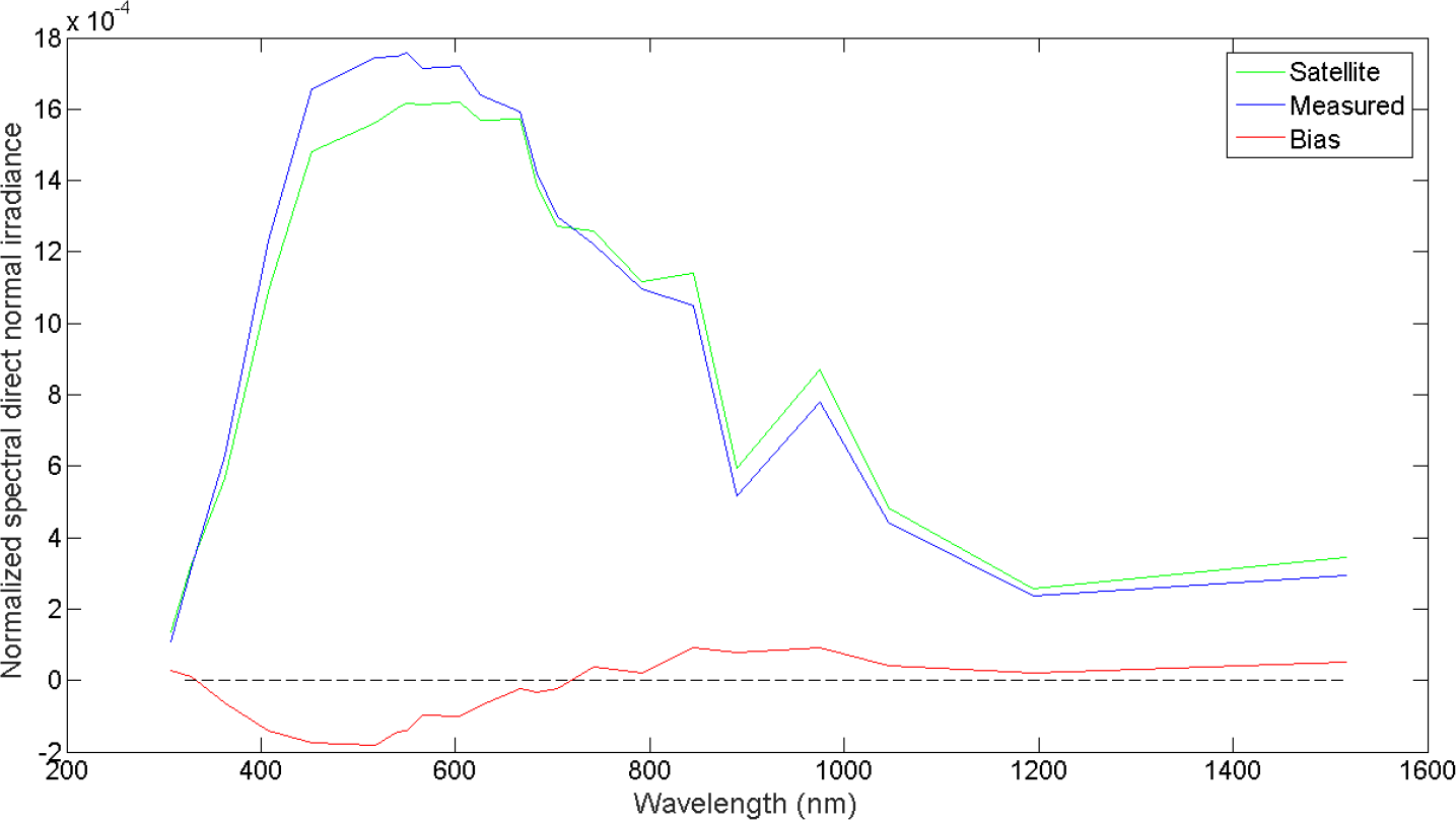
• normalized spectral irradiance R_n (1/nm), obtained by dividing the irradiance value in every Kato band by the sum of the irradiance values of all the Kato bands considered. In this way, the broadband irradiance, after the normalization, is equal to 1 W/m² for both the measurements and the estimates. These relative irradiance values per Kato band make it possible to see if some parts of the estimated spectrum have an excess or deficit relative to the measured averaged spectrum.

In the next two sections, the results of the validation of the estimated global horizontal and direct normal irradiance are presented. Two statistics are applied, general mean bias deviation gMBD and relative general mean bias deviation rgMBD. The general mean bias deviation (gMBD, W/m²) is calculated as the difference between the total irradiance estimated by the SPECMAGIC algorithm for all of the considered Kato bands (K) and the total measured irradiance, according to Equation (9).

$$gMBD={\displaystyle \sum _{i=K_1}^{K_2}{G}_i^{sat}}-{\displaystyle \sum _{i=K_1}^{K_2}{G}_i^{meas}}$$

(9)

where $G_i^{sat}$ and $G_i^{meas}$ are, respectively, the average irradiance in the Kato band i from the satellite database and the measured one (W/m²). K₁ and K₂ are the first and last of the Kato bands available in the considered measured datasets of global horizontal and direct normal irradiance.

The relative general mean bias deviation (rgMBD) is the result of dividing gMBD by the sum of the average measured irradiance in every Kato band considered, following Equation (10).

$$rgMBD=\frac{gMBD}{{\displaystyle {\sum }_{i=K_1}^{K_2}{G}_i^{meas}}}$$

(10)

In addition to these, the mean bias deviation in absolute and relative terms is calculated for every Kato band separately. Other statistics have been calculated, as well, like the root mean square deviation (RMSD) or the mean absolute bias (MAB), but are provided as extra information in the Supplementary Material [37].

4.1. Global Horizontal Radiation

From the initial database for Ispra with measurements at more than 10,000 time points, after applying the process described above to select the closest moments to the available satellite data for this location, the validation of the SPECMAGIC results is performed using 3252 time points. Due to the wavelength range measured of global horizontal irradiance, it is only possible to analyze the Kato bands from 7–27, which cover the wavelength range between 407.5 nm–2153.5 nm. The gMBD of 17.58 W/m², 6.12% in rgMBD, shows that the algorithm tends to overestimate the solar resource in this location. This same trend was observed when the same algorithm was applied to estimate the broadband global horizontal irradiance in the same location [21]. In that other validation, for which data registered in 2005 were used, the resulting errors of 13.85 W/m² gMBD or 9.02% in rgMBD are similar to the deviations shown in the present paper. It should be noted that in the analysis performed in [21], the Ispra location showed the highest annual bias out of 16 stations.

Table 3. Average global horizontal measured spectral irradiance and bias values between satellite and measured databases calculated for the spectral irradiance and normalized values. MBD, mean absolute bias; rMBD, relative MBD.

	Kato Band		Spectral Irradiance, Rλ			Normalized Irradiance, Rn
	Lower Limit (nm)	Upper Limit (nm)	Average Meas (W/m2/nm)	MBD (W/m2/nm) 10−2	rMBD (%)	MBD (1/nm) 10−5	rMBD (%)
7	407.5	452.0	0.42	4.5	10.9	6.6	4.5
8	452.0	517.7	0.50	4.1	8.1	3.3	1.9
9	517.7	540.0	0.49	3.8	7.7	2.6	1.5
10	540.0	549.5	0.49	4.0	8.2	3.3	1.9
11	549.5	566.6	0.48	4.1	8.6	3.9	2.3
12	566.6	605.0	0.46	5.0	10.8	7.0	4.4
13	605.0	625.0	0.45	4.5	10.1	5.8	3.7
14	625.0	666.7	0.43	3.8	8.6	3.6	2.4
15	666.7	684.2	0.44	2.6	5.9	−0.3	−0.2
16	684.2	704.4	0.39	1.8	4.6	−1.9	−1.4
17	704.4	742.6	0.37	1.9	5.2	−1.1	−0.9
18	742.6	791.5	0.34	1.8	5.2	−1.1	−0.9
19	791.5	844.5	0.31	1.5	4.9	−1.2	−1.2
20	844.5	889.0	0.30	1.4	4.8	−1.3	−1.3
21	889.0	974.9	0.17	1.3	7.9	1.0	1.7
22	974.9	1,045.7	0.22	1.1	4.8	−0.9	−1.2
23	1,045.7	1,194.2	0.13	0.4	2.7	−1.4	−3.2
24	1,194.2	1,515.9	0.064	0.2	3.2	−0.6	−2.7
25	1,515.9	1,613.5	0.074	0.5	6.9	0.2	0.8
26	1,613.5	1,964.8	0.029	−0.2	−7.3	−1.3	−12.7
27	1,964.8	2,153.5	0.020	−0.03	−1.7	−0.5	−7.3

contains the results obtained for every Kato band considered. The average measured global horizontal spectral irradiance value (R_λ) along with the bias in absolute MBD (W/m²/nm) and relative terms rMBD (%) are shown. The same statistics are shown for the validation performed on the normalized irradiance values.

Considering the spectral irradiance values in each Kato band, the bias remains below 11% for every band. The highest deviations are observed below 667 nm (Kato band 14). Above that wavelength, the deviations decrease to the point of becoming negative for the last two bands (wavelengths above 1613 nm), even though the width of the bands is considerable bigger than for the first bands.

Using the normalized values, the share of the irradiance contained in every band can be analyzed. As shown in the last two columns in Table 3, the satellite’s estimate results in a distribution of the spectral irradiance that gives more weight to the visible range than there is in the measured spectrum. Conversely, for wavelengths above 700 nm, the estimated values represent a lower share of the broadband irradiance. This is not the case for Kato Bands 21 and 25, which cover a wavelength range affected by the water vapor absorption, that show a positive bias. This could mean that the SPECMAGIC algorithm underestimates this effect for the Ispra site or that the input data related to this effect are not accurate enough for this particular location. However, it should be noted that apart from the two last bands, the relative bias is less than 5% in all considered Kato bands.

Figures 2 and 3 show the satellite and measured spectral and normalized irradiance values per Kato band, along with the corresponding bias (MBD). The satellite and measured values for the different Kato bands are assigned to the mid-wavelength of every band (X axis). For the spectral irradiance (Figure 2), there is a positive bias over nearly the entire spectrum, consistent with the positive bias observed in the broadband irradiance analysis. In contrast, the normalized spectral irradiance shows much better agreement between measured and estimated spectrum, with a positive bias of 2%–5% around 500–800 nm and a slight negative bias beyond 1200 nm.

Similarly to the validation performed on the broadband irradiance [21], data corresponding to clear sky conditions and overcast situations have been analyzed separately also for the spectrally-resolved irradiance. The results are presented in the Supplementary Material [37].

4.2. Direct Normal Radiation

From the initial database for Nicosia with more than 7,000 time points, once the measured values are integrated into Kato bands and the closest moments to the available satellite data have been selected, the validation of the algorithm is performed using 790 time points. Due to the wavelength range measured of direct normal irradiance, it is only possible to analyze the Kato bands from 4–25, which cover the wavelength range from 306.8–1613.5 nm.

The general bias, gMBD, of 34.6 W/m² is higher than the one obtained in the validation of the global horizontal irradiance. However, due to the higher direct irradiance values at this site, the relative bias of 6.49% rgMBD is similar in both datasets. The positive bias in the broadband irradiance is also observed over most of the wavelength range in the spectral direct irradiance. These results agree with those obtained in the first validation of the SPECMAGIC algorithm, being a bit higher than those reported in [13]. The accuracy observed on that occasion was in the range of the uncertainty of surface measurements, which is about 5%, with the exception of the part of the spectrum above 1200 nm (Kato Band 24 and above), where higher deviations were observed.

Table 4. Average direct normal measured spectral irradiance and bias values between satellite and measured databases calculated for the spectral irradiance and normalized values.

	Kato Band		Spectral Irradiance, RDNI,λ			Normalized Irradiance, RDNI,n
	Lower Limit (nm)	Upper Limit (nm)	Average Meas (W/m2/nm)	MBD (W/m2/nm) 10−2	rMBD (%)	MBD (1/nm) 10−5	rMBD (%)
4	306.8	327.8	0.06	1.9	32.7	2.7	24.6
5	327.8	362.5	0.17	1.7	10.4	1.1	3.6
6	362.5	407.5	0.34	−1.4	−4.1	−6.3	−9.9
7	407.5	452.0	0.66	−3.7	−5.7	−14.0	−11.4
8	452.0	517.7	0.88	−4.2	−4.8	−17.5	−10.6
9	517.7	540.0	0.93	−4.2	−4.5	−18.0	−10.3
10	540.0	549.5	0.93	−2.2	−2.4	−14.5	−8.3
11	549.5	566.6	0.94	−1.9	−2.1	−14.1	−8.0
12	566.6	605.0	0.91	0.3	0.4	−9.9	−5.8
13	605.0	625.0	0.92	0.2	0.2	−10.0	−5.9
14	625.0	666.7	0.87	1.7	2.0	−6.9	−4.2
15	666.7	684.2	0.85	4.3	5.0	−2.2	−1.4
16	684.2	704.4	0.76	3.0	4.0	−3.3	−2.3
17	704.4	742.6	0.69	3.1	4.5	−2.4	−1.9
18	742.6	791.5	0.65	6.3	9.8	3.7	3.1
19	791.5	844.5	0.58	5.0	8.5	2.0	1.9
20	844.5	889.0	0.56	8.9	15.9	9.2	8.8
21	889.0	974.9	0.27	6.2	22.5	7.8	15.1
22	974.9	1,045.7	0.42	7.9	19.0	9.2	11.8
23	1,045.7	1,194.2	0.23	3.9	16.5	4.2	9.4
24	1,194.2	1,515.9	0.13	2.0	15.8	2.1	8.8
25	1,515.9	1,613.5	0.16	3.9	25.1	5.1	17.5

contains the results obtained for every considered Kato band in the estimation of the direct normal irradiance (R_DNI,λ). The average measured spectral irradiance value, along with the bias in absolute MBD (W/m²/nm) and relative terms rMBD (%) are shown. The same statistics are shown for the validation performed on the normalized irradiance values.

The results obtained for the spectral direct irradiance show a tendency to underestimate the part of the spectrum below 566 nm with the exception of the first two available bands and to overestimate the rest of the wavelength range measured. The bias for the various Kato bands are generally higher than the ones obtained for the global horizontal irradiance. However, the relative mean bias deviation values are similar in both datasets.

The same trend to underestimate in the lowest part of the spectrum and overestimate in higher wavelength ranges is also observed when considering the normalized values. This is the opposite of what was observed for the global horizontal spectral irradiance.

Figures 4 and 5 show, respectively, the satellite and measured spectral and normalized irradiance values per Kato band, along with the corresponding bias.

In both figures, a significant overestimation is noticeable at wavelengths above 1200 nm, as was observed also by Müller et al. [13], in the first validation of the SPECMAGIC algorithm.

Due to the small number of months analyzed and the fact that direct normal irradiance is very low in the case of overcast sky conditions, the validation of the algorithm has not been performed selecting clear and overcast sky conditions, as has been done for the global horizontal irradiance.

4.3. Average Photon Energy Calculation

The average photon energy can be used to describe the spectral irradiance distribution at a certain location to within a level of certainty, as shown by Minemoto et al. [12,35]. Despite the applications of the APE values and due to the lack of spectrally-resolved irradiance data, in this section, we have calculated the APE values considering the output of the SPECMAGIC algorithm. In order to validate the suitability of considering those satellite-based values for the APE calculation, we have calculated the APE with three different datasets:

• global horizontal spectral irradiance measured every 2 nm (meas);
• global horizontal spectral irradiance measured every 2 nm, but integrated into Kato bands (measKB);
• satellite-derived global horizontal spectral irradiance, which is already integrated into Kato bands (satKB).

By comparing the first two, we can analyze whether the integration of the spectral irradiance into Kato bands affects the APE values that would result from considering the real measurements recorded every few nm. Comparing the APE values resulting from the last two datasets will help with analyzing the suitability of the satellite data for the estimation of the APE values at a certain location. The data used for this analysis, both measured and satellite-based values, correspond to Ispra (Italy) and were used in previous sections. A total number of 3252 data points have been considered, as explained in Section 4.1. For the estimation of the APE values, only the wavelength range between 400 nm and 1050 nm is used, which covers the Kato bands from 7–22, inclusive. A full description of the calculation procedure for the APE can be found in Norton et al. [35].

The APE values for the three datasets are shown in

Table 5. Average photon energy (APE) values calculated for the spectral global horizontal irradiance values measured and estimated for Ispra, using data from January 2009 to June 2010.

Dataset	APE Value
Meas	1.8468
MeasK B	1.8409
SatK B	1.8477

, while the average monthly APE values for the three datasets are shown in Figure 6.

Calculating the APE values using the measured data integrated into Kato bands (MeasKB) reduced the APE values by about 0.32% with regard to the values obtained when considering the measurements recorded every 2 nm (Meas). When APE values are calculated using the satellite retrieved values, APE tends to be higher than those obtained from the measured data, especially for the winter months (from October–February). However, considering the yearly average values, both APE values from MeasKB and SatKB are very similar, with a bias of 0.37%. This is consistent with the results shown in Figure 3 that showed a slight positive bias in the blue end of the spectrum, leading to a higher APE. In view of these results, we can conclude that the SPECMAGIC output values could well be applied to estimate the APE values at any location.

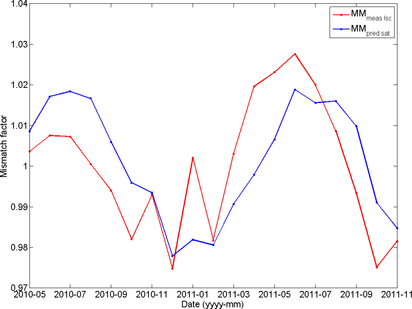
4.4. Validation of the Model for PV Performance under Varying Spectrum

The ability of the algorithm to retrieve spectral irradiance values from satellite images has been validated in the previous sections. In this section, these satellite values will be applied to validate the model used to estimate the changes in the performance of PV modules under different solar spectra. For this, outdoor measurement data from a CdTe module will be used.

The PV module considered was measured outdoors during the period of time between May 2010, and November, 2011, in the test installation at the Joint Research Centre (JRC) ESTI Laboratory located in Ispra, Italy. The measurement system for long-term outdoor measurements of PV modules is described in [38] (see also [4]). The PV modules are mounted on a metal rack facing south at an inclination angle of 45° from the horizontal plane. The module temperatures, T_mod, are measured by PT100 sensors on the back of the modules. The in-plane of array irradiance, G_POA, is measured using a calibrated silicon reference cell mounted in the same plane as the modules. Measurements are made approximately every four minutes during daytime, provided the in-plane irradiance exceeds the threshold of 50 W/m².

To validate the spectral performance model, the effective long-term mismatch factor for the CdTe module, MM_CdTe, is calculated using both satellite-derived irradiance data and real measurements of the module short-circuit current. First, the spectral mismatch factor for I_sc, MM_Isc,n, is calculated by inserting the module short-circuit current data for each measurement moment n into Equation (3). The measured module short-circuit current, I_sc, at each moment must be corrected to a temperature of 25°C. This is done according to Equation (11), where α is the temperature coefficient of the module, and T_mod (°C) is the module temperature. α was found from indoor measurements to have the value of α = −0.00055 °C⁻¹.

$$I_{sc\_25}=\frac{I_{sc}}{1-(\mathrm{\alpha }\cdot (T_{mad}-25°\mathrm{C}))}$$

(11)

The overall spectral mismatch factor 〈MM_{meas_Isc}〉 can then be calculated in the following way (similar to [6,8]). In the absence of spectral effects, the short-circuit current would be proportional to the measured irradiance: I_sc = (G_POA/G_STC) · I_{sc_STC}, where I_{sc_STC} is the short circuit current under STC conditions and G_STC is the STC irradiance of 1000 W/m². The instantaneous spectral mismatch factor is then calculated as the deviation of the measured I_sc from this “ideal” value:

$$M{M}_{Isc,n}=I_{sc}\cdot G_{\mathrm{STC}}/(G_{POA}\cdot I_{sc\_STC})$$

I_{sc_STC} was found from the outdoor measurements using the (temperature-corrected) I_sc values during times when G_POA ≃ 1000 W/m² and the air mass AM ≃ 1.5.

The overall measured spectral mismatch for the time period of the measurements is then calculated using Equation (12):

$$\langle M{M}_{\mathrm{meas}\_Isc}\rangle =\frac{{\displaystyle {\sum }_{n=1}^{N}M{M}_{Isc,n}\cdot I_{sc\_25,n}}}{{\displaystyle {\sum }_{n=1}^N{I}_{sc\_25,n}}}$$

(12)

To estimate the overall mismatch factor for CdTe using the satellite data, 〈MM_{CdTe_sat}〉, the instantaneous spectral correction factor MM_{CdTe_sat,n} for each measurement moment n is first calculated by inserting the satellite spectral irradiance data R_SAT (λ) and the CdTe module spectral response, S_r,CdTe(λ), into Equation (3). The mismatch factor for the entire measurement period is then calculated by summing these values weighted by the irradiance intensity at which they occur, as described in Equation (13):

$$\langle M{M}_{\mathrm{CdTe}\_sat}\rangle =\frac{{\displaystyle {\sum }_{n=1}^{N}M{M}_{\mathrm{CdTe}\_sat,n}}\cdot G_{POA,n}}{{\displaystyle {\sum }_{n=1}^N{G}_{POA,n}}}$$

(13)

here, G_POA,n is the plane-of-array irradiance, in this case measured using a calibrated silicon reference cell. However, this approach introduces an additional calculation step, because this reference cell has its own spectral mismatch value. To correct for this, it is necessary to divide the satellite mismatch value for the CdTe module, 〈MM_{CdTe_sat}〉, by the mismatch of the silicon reference cell, 〈MM_{Si_sat}〉, as shown in Equation (14).

$$\langle M{M}_{\mathrm{pred}\_sat}\rangle =\frac{\langle M{M}_{\mathrm{CdTe}\_sat}\rangle }{\langle M{M}_{\mathrm{Si}\_sat}\rangle }$$

(14)

Here, 〈MM_{pred_sat}〉 is the predicted overall mismatch between the CdTe module and the irradiance measured by the Si reference cell. 〈MM_{Si_sat}〉 is calculated in the same manner as for 〈MM_{CdTe_sat}〉, but inserting the satellite irradiance data R_SAT (λ) and the Silicon reference cell spectral response, S_r,Si(λ), into Equation (3), to calculate for every moment n for the spectral mismatch factor MM_{Si_sat,n}.

For the period of time the CdTe module was measured outdoors, there are approximately 35,000 satellite data points and 100,000 measurements from the outdoor field. In order to perform the validation of the model in the most accurate way and considering the frequency of the measurements from the outdoor field, only those data from the satellite and the outdoor field datasets, whose time difference was below five minutes, were selected. In the end, almost 10,000 data points are used for this analysis.

For a given moment n, three different spectral correction factors are calculated (MM_Isc,n, MM_{CdTe_sat,n} and MM_{Si_sat,n}). From these values, the overall mismatch factors are calculated (〈MM_{meas_Isc}〉, 〈MM_{CdTe_sat}〉 and 〈MM_{Si_sat}〉; with these last two values, 〈MM_{pred_sat}〉 is calculated). The results of these calculations are shown in

Table 6. Mismatch factors obtained for the CdTe module using measured and estimated input data. Weighted average for the measurement period May, 2010–November, 2011.

Mismatch Factor	Value (%)
Predicted CdTe mismatch 〈MMCdTe_sat〉	1.00
Predicted Si mismatch 〈MMSi_sat〉	0.61
Predicted mismatch between CdTe and Si sensor 〈MMpred_sat〉	0.39
Measured mismatch between CdTe and Si sensor 〈MMmeas_Isc〉	0.30

.

Both mismatch values (〈MM_{meas_Isc}〉 and 〈MM_{pred_sat}〉) show that, for the location analyzed, the effective irradiance, G_eff, received by the CdTe module would be slightly higher than the in-plane of array irradiance registered in the measured database, G_POA. This would improve the estimated performance of the module for this location with regard to the estimations obtained if the spectral effect were not taken into account. Considering the mismatch factor resulting from the measurements as the real value for the module, 〈MM_{meas_Isc}〉, using the satellite data to estimate the effective irradiance would imply an overestimation of 0.09%. This result shows that using the satellite information provides accurate results, at least for the location analyzed. However, it would be necessary to consider other PV technologies, as well as data from other locations.

The comparison of the mismatch factors has also been made month by month. The numbers are provided in Supplementary Material [37]. Figure 7 shows the monthly variation in the mismatch factors. It can be seen that the annual variability is higher for the ground-based measurement values than for the satellite-based values.

The spectral mismatch shows a clear variation over the seasons, with generally higher values in summer and lower values in winter. This pattern is found both in the ground-based data (〈MM_{meas_Isc}〉) and in the satellite estimates values (〈MM_{pred_sat}〉). In most cases, both values tend to agree, in the sense that both are above or below one simultaneously. As was shown above, when considering the whole time period, the satellite estimate of the mismatch factor is only slightly higher than that obtained from the I_sc measurements. However, when looking at monthly values, there are larger deviations. Considering the common available months in the two years (from May–November), the satellite-based estimates for a given month are more similar between the years than the ground-based calculation. This may indicate a problem either with the measurements of the irradiance or in the measurement of I_sc. If this is the case, the main conclusion must be that the difference between the satellite-based and ground-based calculation is well within the uncertainty of the ground-based measurements. However, this comparison does show that the satellite-based estimate can resolve the variations in the mismatch over the seasons, which is an indication that the method can work over a range of different conditions (different weather types and varying Sun elevation angles). Considering the satellite data results in a general overestimation of the mismatch factor (〈MM_{pred_sat}〉 > 〈MM_{meas_Isc}〉). However, there are some months, around the winter period, where an underestimation is observed. The bias varies between −2.13% and 1.66%, although for half of the months, the bias remains below 1%.

5. Geospatial Mapping of PV Performance Variations due to Solar Spectrum Variations

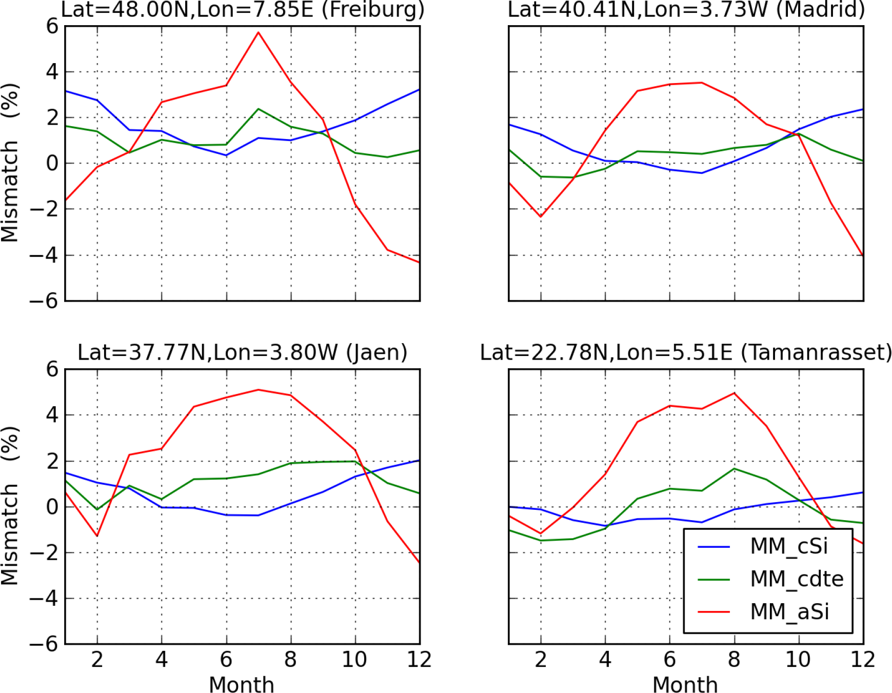
5.1. Comparison with Results from the Literature

The validation presented in the previous section suffers from the fact that actual measured data for PV modules were available for only one single site. It would therefore be useful to compare the results we have obtained with those published by other groups. It will not be a true validation, since there are a number of differences in the approaches, but it will still be useful to see how well these studies compare.

Two recent studies have reported values for the spectral mismatch of different module types at various locations: Alonso-Abella et al. [6] and Dirnberger et al. [8]. In the first study, four different sites in Germany, Spain and Algeria were used, while the second study reports results for Freiburg, Germany.

There are a number of differences in approaches, which means that the comparison will not be exact. The two studies considered an inclination angle of 30°, while our results are for 20° inclination. Especially for a-Si, the spectral response varies between manufacturers, and the one used in [8] seems to have a slightly broader spectral response curve. The time period is different, and the results in [8] show some variation between years. Finally, these two studies considered only the influence of the spectrum on I_sc, and the mismatch is essentially the deviation in monthly or annual average I_sc. In contrast, our study uses the spectrally-corrected irradiance as input to a model for the module power. If there is a correlation between module temperature and the spectral effect (and this can be seen in the seasonal variation in Figure 7), the overall mismatch in the energy produced will be different from that considering only I_sc.

Both studies have presented results as monthly average mismatch for the different PV technologies and locations. Figure 8 below shows similar results for four different locations: Freiburg [8] and Madrid, Jaen and Tamanrasset [6].

A comparison with the results of the previous studies shows that there are strong similarities: the seasonal variation of a-Si is stronger than for the other two module types; peak positive mismatch for a-Si is in summer for all four sites, while the a-Si mismatch is slightly negative in winter. The spectral effect is smaller for CdTe and c-Si, and there is less seasonal variation.

Some differences are also evident: our results show a somewhat stronger seasonal effect for c-Si than the other studies, with the lowest values in summer. The overall effect for c-Si is stronger than the values found in [6]. For CdTe, the seasonal variation is less clear in our results, and the overall effect is somewhat lower than the one found in [8].

Table 7. Annual average mismatch 〈MM〉 (in percent) for four different locations and three different PV technologies. The comparison is between the results obtained in this work compared with values found in recent studies.

Location	This Work			Recent Studies [6,8]
	c-Si	CdTe	a-Si	c-Si	CdTe	a-Si
Freiburg	+1.3	+1.1	+2.0	+1.4	+2.4	+3.4
Stuttgart	+1.3	+1.1	+1.8	−0.6	−0.5	−0.4
Madrid	+0.6	+0.4	+1.3	+0.6	−1.2	−0.5
Jaen	+0.5	+0.6	+2.8	−0.2	−0.4	0.4
Tamanrasset	−0.2	−0.1	+1.7	−0.8	+0.1	+2.2

shows annual average mismatch for the three PV technologies for five locations, comparing our results with those of [6,8]. In the table, also Stuttgart is shown [6]. Our results differ from these authors by up to ±2%. Given the differences in approaches, this is not surprising. An interesting case is the values from Freiburg and Stuttgart, which are geographically close. Here, our results show very similar values, while the results of [8] (Freiburg) and [6] (Stuttgart) vary more between each other and in opposite directions from our results ([8] shows higher values of 〈MM〉, while [6] has lower values).

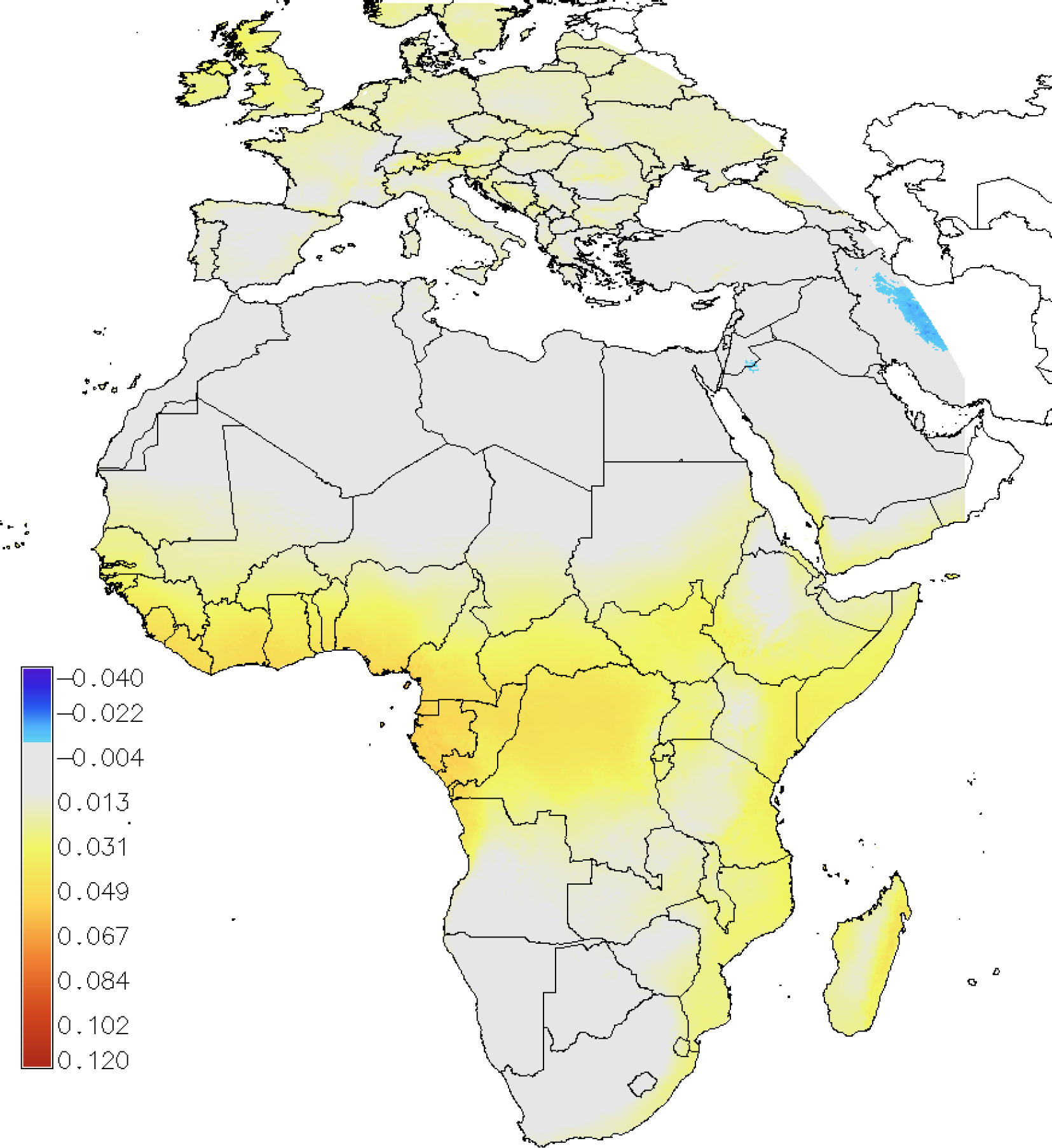
5.2. Mapping the Influence of the Spectrum on PV Performance

Using the data and models described in Sections 2 and 3, it is now possible to estimate the performance of different PV module types over large geographical regions. The calculations are performed to obtain estimates of the PV power output at each hour of a year, using the following steps:

• From the global horizontal and direct horizontal irradiance, calculate the inclined-plane direct and diffuse irradiance in each spectral band (Section 2.2).
• Correct the in-plane of array irradiance for AOI effects (Section 3.1).
• From the corrected direct and diffuse irradiance, use Equation (3) to calculate the effective irradiance.
• Calculate the module temperature from the AOI-corrected irradiance, ambient temperature and wind speed using Equation (8).
• Use Equations (5)–(7) to calculate the instantaneous module power.

In order to estimate the overall effect of spectral variations, we have also performed these calculations leaving out Step 3 in the list above, so the power will be estimated without taking into account the solar spectrum.

The calculation steps in the above list have been performed using one year of irradiance data derived from the Meteosat-7 satellite at 0° longitude. The coverage area of this satellite is Europe, Africa and parts of western Asia. Temperature and wind data were taken from the European Centre for Medium-Range Weather Forecast (ECMWF) ERA-Interim reanalysis, with a spatial resolution of 0.75° latitude/longitude and a time resolution of 3 h [39]. The study year is 2005. For this calculation, the modules were assumed to be mounted on a fixed open-rack facing the Equator at an inclination angle of 20° from the horizontal plane.

The resulting maps show the estimated total energy production by a 1kW_p array of modules of the given module type. The annual energy production E_tot,spec is calculated following Equation (15):

$$E_{\mathrm{t}ot,spec}={\displaystyle \sum _{t_h=1}^{8760}P(G_{eff}(t_h),T_{mod}(t_h))}$$

(15)

where t_h is the h-th hour in the year.

An example of these maps of annual energy PV output is shown in Figure 9, where the PV output estimation for a CdTe module is calculated for the year 2005 considering the effects of irradiance and temperature on PV performance, as well as the spectral effects.

A similar map was calculated for the total energy E_tot, but leaving out the spectral correction step (Step 3 in the above list). From these two energy output estimates, we can then calculate a measure of the annual average spectral mismatch, 〈MM〉 (Equation (16)):

$$\langle MM\rangle =\frac{E_{\mathrm{t}ot,spec}-E_{\mathrm{t}ot}}{E_{\mathrm{t}ot}}$$

(16)

A map of 〈MM〉 for CdTe modules is shown in Figure 10. From the figure, we see that in large regions, the spectral effect is very small. This is the case in desert areas (north Africa, Arabia and Namibia) and in Southern Europe (Turkey, southern Spain). In most of Europe, the effect is a little larger, at around 0.01–0.02 (corresponding to 1%–2% extra energy output), increasing as we move north. The largest effect is seen in humid tropical regions, such as equatorial West Africa, where the effect can be up to about 0.05 (5% extra energy). The region with a negative spectral effect at the easternmost edge of the image is probably an artifact caused by the increased uncertainty in the solar radiation estimates at the edge of the satellite image.

The same calculation was carried out also for crystalline silicon modules and for a single-junction amorphous silicon module (see the spectral response curves in Figure 1). The results are shown in Figures 11 and 12 respectively, showing again the spectral effect as calculated in Equation (16). The color scale is the same in Figures 10–12 to make the comparison easier.

It is clear from Figure 11 that the influence of the spectral variations is much less pronounced for crystalline silicon modules. In all of Africa and in Southern Europe, the absolute value of the effect is less than 1%. In Central Europe, this increases somewhat to about +2%, and the strongest effect is found in Northern Europe, but the effect is still limited to about +3%.

In contrast, the effect of the spectral variations is much more pronounced for amorphous silicon (Figure 12). The effect is nearly always positive, again with the lowest values found in desert areas (from 0 to +2%). In Europe, the effect is somewhat stronger, at +3% or +4%. As for CdTe, the strongest effect is found in the tropical areas of Africa, where the effect may reach as high as +10%, meaning that the actual energy output of the module may be up to 10% higher than would be predicted without taking into account the spectral effects.

The overall pattern of the effects is that the effect is stronger in areas with a high level of diffuse irradiance, such as northern Europe and tropical West Africa. The effect is also stronger for PV technologies with more narrow spectral response curves, with the strongest effect seen for amorphous silicon that is only sensitive to radiation with a wavelength less than 750 nm.

5.3. Spectral Effect Dependence on Inclination Angle

The results shown in the previous section have all been calculated using a single inclination angle for the PV modules (20° from the horizontal plane, Equator-facing). If the inclination angle is changed, the amount of in-plane irradiance changes, but also the ratio of direct to diffuse irradiance is affected. In order to study the effect of changing inclination angle, we have performed the calculation of MM for a number of different inclination angles for four different locations. These locations represent a humid equatorial climate, Köppen–Geiger (K-G) classification “Aw” (1°48′N, 15°20′E), a desert climate, K-G= “BWh” (24°55′N, 46°25′E), a Mediterranean climate, K-G = “Csa” (44°5′N, 5°4′E), and a maritime Northern European climate, K-G = “Cfb” (51°97′N, 4°56′E). The inclination angle was varied from 0° to 60°, south-facing. The calculation was made for one year (2011) for three different module types. The resulting values of MM are shown in Figure 13.

The spectral performance of c-Si modules varies only slightly with inclination angle. The effect is somewhat more pronounced for CdTe and even more for single-junction a-Si. Furthermore, at latitudes close to the Equator, the tendency is towards an increased effect at steep inclinations, while at more northerly locations, the variation is in the opposite direction. This may be due to the changing ratio of direct to diffuse light. Near the Equator, the amount of direct sunlight decreases with increasing inclination, while at higher latitudes, the amount of direct light increases (until the inclination angle equals the latitude) while the diffuse light decreases.

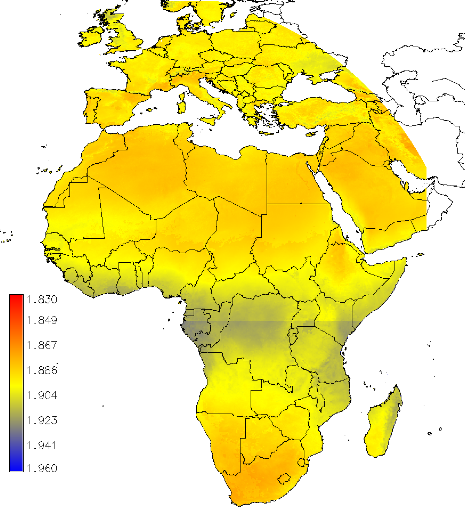
5.4. Mapping Average Photon Energy

The average photon energy (APE) is one way to reduce the complexity of variations in the spectrum of sunlight to a single parameter. As the name implies, this number is simply the average energy of the photons arriving in a given plane located at the Earth’s surface within a given time period. The averaging may be performed for all of the wavelengths in the sunlight or may be restricted to a certain band.

In the study presented here, APE has not been used to estimate PV performance, as the full spectrum information is available from the satellite-based estimates. However, it could still be useful to calculate APE in order to compare these results with other studies.

The annual average APE was calculated for irradiance in the same plane (20° Equator-facing) as the results shown in the previous sections. For the present study, we chose the interval 300–1050 nm for the calculations. In each spectral band, the photon energy is assumed to be equal to that of the central wavelength in that band.

The annual average of APE can then be found as an irradiance-weighted average of the hourly APE maps, according to Equation (17):

$$\langle APE\rangle =\frac{{\displaystyle {\sum }_{t_h=1}^{8760}AP{E}_{t_h}\cdot G_{POA,t_h}}}{{\displaystyle {\sum }_{t_h=1}^{8760}{G}_{POA,t_h}}}$$

(17)

The resulting map of APE for the year 2005 is shown in Figure 14.

It is clear from the map that the overall pattern of variation in APE is similar to the pattern of PV performance variations shown in Figures 10–12, especially for the PV technologies with the most restricted spectral range. However, these maps will not by themselves show how good is the correlation between APE and the mismatch factor or whether APE can be used to predict MM with reasonable accuracy. A detailed discussion of this is outside the scope of this paper, but a few examples will be shown to give an idea of the issue. Figure 15a shows the instantaneous values of MM for a-Si for a location in Gabon. Figure 15b shows 〈MM〉 values for CdTe for 1,000 random locations in the study area.

While it is clear that there is indeed some relation between APE and MM, it is also clear from the figures that there is quite a lot of variation in both MM and 〈MM〉 for any given value of APE. Thus, MM for a-Si at this location may vary by almost ±10% for the same APE. This range is almost twice as high as the range of values of 〈MM〉 for a-Si in the whole study area. For the 〈MM〉 of CdTe, the values at different locations with the same average APE may vary by up to three percentage points, which is about half the total range of 〈MM〉 for CdTe.

These results show that at least in these cases, APE would not be a good indicator of the spectral mismatch of PV systems. In addition, there is the problem that APE must be estimated in some way for all locations where solar spectral measurements are not available, which would introduce a further uncertainty in the estimate of the mismatch. For these reasons, we would suggest that it is preferable to use spectrally-resolved radiation data from satellites to estimate the spectral mismatch for PV studies, if these data are available.

6. Conclusions

We have presented a method for calculating the effect of time-varying sunlight spectrum on the performance of PV modules using spectrally-resolved irradiance data estimated from satellite data. The satellite data necessary for the method may be calculated from the Meteosat satellites covering Eurasia and Africa.

Validation of the satellite-based spectral data performed in previous papers and in this study shows that the agreement between estimated and measured spectral data is good, both for the spectrum of global horizontal irradiance and direct normal irradiance. The method to estimate the spectral effect on PV modules was also checked against measured data from a CdTe module and found to give good agreement.

Applying spectral response data for crystalline silicon, CdTe and single-junction amorphous silicon modules to the spectral satellite data, we were able to construct maps of the annual average spectral effect on these module types over Europe and Africa. Generally, the effect is small for all three module types in desert areas, indicating that the average spectrum here is quite close to the standard spectrum. A small positive effect of +2 to +4% is seen in most of Central and Northern Europe for CdTe and a-Si modules. The strongest effect is seen in tropical Africa, where CdTe modules may produce up to about 6% more energy due to spectral effects, while for a-Si modules, the effect may reach +10%. In contrast, in this area, c-Si modules show little overall effect. The magnitude of this effect is large enough that it should be taken into account when estimating PV energy production in these areas.

For the time being, the study has been performed only for single-junction PV technologies, such as crystalline silicon, CdTe or single-junction a-Si modules. Multijunction PV technologies have a more complicated behavior under varying spectra due to the varying spectral sensitivity of the different layers. This study also considered only fixed-mounted flat-plate PV modules. Concentrating PV modules use only the direct normal irradiance, which will have a different spectrum, and, also, often use multijunction cells. We plan to use the methods developed for this study to investigate the spectral effects for these PV technologies in the near future.

References

1. Gottschalg, R.; Infield, D.G.; Kearny, M.J. Experimental study of variations of the solar spectrum of relevance to thin film solar cells. Solar Energy Mater. Solar Cells 2003, 79, 527–537. [Google Scholar]
2. Gottschalg, R.; Betts, T.R.; Williams, S.R.; Sauter, D.; Infield, D.G.; Kearny, M.J. A critical appraisal of the factors affecting energy production from amorphous silicon photovoltaic arrays in a maritime climate. Solar Energy 2004, 77, 909–916. [Google Scholar]
3. Minemoto, T.; Nagae, S.; Takakura, H. Impact of spectral irradiance distribution and temperature on the outdoor performance of amorphous Si photovoltaic modules. Solar Energy Mater. Solar Cells 2007, 91, 919–923. [Google Scholar]
4. Nikolaeva-Dimitrova, M.; Kenny, R.; Dunlop, E.; Pravettoni, M. Seasonal variations on energy yield of a-Si, hybrid, and crystalline Si PV modules. Prog. Photovolt. Res. Appl. 2010, 18, 311–320. [Google Scholar]
5. Gottschalg, R.; Betts, T.R.; Eeles, A.; Williams, R.R.; Zhu, J. Influences on the energy delivery of thin film photovoltaic modules. Solar Energy Mater. Solar Cells 2013, 119, 169–180. [Google Scholar]
6. Alonso-Abella, M.; Chenlo, F.; Nofuentes, G.; Torres-Ramirez, M. Analysis of spectral effects on the energy yield of different PV (photovoltaic) technologies: The case of four specific sites. Energy 2014, 67, 435–443. [Google Scholar]
7. Nofuentes, G.; Garcia-Domingo, B.; Munoz, J.V.; Chenlo, F. Analysis of the dependence of the spectral factor of some PV technologies on the solar spectrum distribution. Appl. Energy 2014, 113, 302–309. [Google Scholar]
8. Dirnberger, D.; Blackburn, G.; Müller, B.; Reise, C. On the impact of solar spectral irradiance on the yield of different PV technologies. Solar Energy Mater. Solar Cells 2015, 132, 431–442. [Google Scholar]
9. Jardine, C.; Betts, T.; Gottschlg, R.; Infield, D.G.; Lane, K. Influence of spectral effects on the performance of multijunction amorphous silicon cells, Proceedings of the 17th European Photovoltaic and Solar Energy Conference, Munich, Germany, 22–26 October 2001; 44.
10. Belluardo, G.; Wagner, J.; Tetzlaff, A.; Moser, D. Evaluation of spectral effect on module performance using modeled average wavelength, Proceedings of the 28th European Photovoltaic Solar Energy Conference and Exhibition, Paris, France, 30 September 2013.
11. Peharz, G.; Siefer, G.; Bett, A.W. A simple method for quantifying spectral impacts on multi-junction solar cells. Solar Energy 2009, 83, 1588–1598. [Google Scholar]
12. Minemoto, T.; Nakada, Y.; Takahashi, H.; Takakura, H. Uniqueness verification of solar spectrum index of average photon energy for evaluating outdoor performance of photovoltaic modules. Solar Energy 2009, 83, 1294–1299. [Google Scholar]
13. Müller, R.; Behrendt, T.; Hammer, A.; Kemper, A. A new algorithm for the satellite-based retrieval of solar surface irradiance in spectral bands. Remote Sens. 2012, 4, 622–647. [Google Scholar]
14. Behrendt, T.; Kuehnert, J.; Hammer, A.; Lorenz, E.; Betcke, J.; Heinemann, D. Solar spectral irradiance derived from satellite data: A tool to improe thin film PV performance estimations? Solar Energy 2013, 98, 100–110. [Google Scholar]
15. Mueller, R.; Trentmann, J.; Träger-Chatterjee, C.; Posselt, R.; Stöckli, R. The role of the effective cloud Albedo for climate monitoring and analysis. Remote Sens. 2011, 3, 2305–2320. [Google Scholar]
16. Morcrette, J.; Boucher, O.; Jones, L.; Salmond, D.; Bechtold, P.; Beljaars, A.; Benedetti, A.; Bonet, A.; Kaiser, J.; Razinger, M.; et al. Aerosol analysis and forecast in the European Centre for Medium-Range Weather Forecasts Integrated Forecast System: Forward modeling. J. Geophys. Res. 2009, 114. [Google Scholar] [CrossRef]
17. Benedetti, A.; Morcrette, J.; Boucher, O.; Dethof, A.; Engelen, R.; Fisher, M.; Flentje, H.; Huneeus, N.; Jones, L.; Kaiser, J.; et al. Aerosol analysis and forecast in the European Centre for Medium-Range Weather Forecasts Integrated Forecast System: 2. Data assimilation. J. Geophys. Res. 2009, 114. [Google Scholar] [CrossRef]
18. Dee, D.; Uppala, S. Variational bias correction of satellite radiance data in the ERA-interim reanalyis. Q. J. R. Meteorol. Soc. 2009, 135, 1830–1841. [Google Scholar]
19. Betts, A.; Ball, J.; Bosilovich, M.; Viterbo, P.; Zhang, Y.; Rossow, W. Intercomparison of water and energy budgets for five Mississippi subbasins between ECMWF re-analysis (ERA-40) and NASA Data Assimilation Office fvGCM for 1990–1999. J. Geophys. Res. 2003, 108. [Google Scholar] [CrossRef]
20. Mayer, B.; Kylling, A. Technical note: The libRadtran software package for radiative transfer calculations-Description and examples of use. Atmos. Chem. Phys. 2005, 135, 1855–1877. [Google Scholar]
21. Gracia Amillo, A.; Huld, T.; Müller, R. A New Database of Global and Direct Solar Radiation Using the Eastern Meteosat Satellite, Models and Validation. Remote Sens. 2014, 6, 8165–8189. [Google Scholar] [Green Version]
22. Kato, S.; Ackerman, T.; Mather, J.; E.E.C. The k-distribution method and correlated-k approximation for a shortwave radiative transfer model. J. Quant. Spectrosc. Radiat. Transf. 1999, 62, 109–121. [Google Scholar]
23. Gueymard, C. Prediction and validation of cloudless shortwave solar spectra incident on horizontal, tilted, or tracking surfaces. Solar Energy 2008, 82, 260–271. [Google Scholar]
24. Šúri, M.; Hofierka, J. A New GIS-based Solar Radiation Model and Its Application to Photovoltaic Assessments. Trans. GIS 2004, 8, 175–190. [Google Scholar]
25. Muneer, T. Solar radiation model for Europe. Build. Serv. Eng. Res. Technol. 1990, 4, 153–163. [Google Scholar]
26. Perez, R.; Seals, R.; Ineichen, P.; Stewart, R.; Menicucci, D. A new simplified version of the Perez diffuse irradiance model for tilted surfaces. Solar Energy 1987, 39, 221–231. [Google Scholar]
27. Martin, N.; Ruiz, J. Calculation of the PV modules angular losses under field conditions by means of an analytical model. Solar Energy Mater. Solar Cells 2001, 70, 25–38. [Google Scholar]
28. Bahrs, U.; Zaaiman, W.; Mertens, M.; Ossenbrink, H. Automatic large area spectral response facility, Proceedings of the 14th European Photovoltaic SolarEnergy Conference, Barcelona, Spain, 30 June–4 July 1997; pp. 2296–2298.
29. King, D.; Boyson, W.; Kratochvil, J. Photovoltaic Array Performance Model; Technical Report SAND2004-3535; Sandia National Laboratories: Albuquerque, NM, USA, 2004. [Google Scholar]
30. Friesen, G.; Chianese, D.; Pola, I.; Realini, A.; A., B. Energy rating measurements and predictions at ISAAC, Proceedings of the 22nd European Photovoltaic SolarEnergy Conference, Milan, Italy, 3–7 September 2007; pp. 2754–2757.
31. Skoplaki, E.; Palyvos, J. On the temperature dependence of photovoltaic module electrical performance: A review of efficiency/power correlations. Solar Energy 2009, 83, 614–624. [Google Scholar]
32. Huld, T.A.; Friesen, G.; Skoczek, A.; Kenny, R.A.; Sample, T.; Field, M.; Dunlop, E.D. A power-rating model for crystalline silicon PV modules. Solar Energy Mater. Solar Cells 2011, 95, 3359–3369. [Google Scholar]
33. Faiman, D. Assessing the outdoor operating temperature of photovoltaic modules. Prog. Photovolt. Res. Appl. 2008, 16, 307–315. [Google Scholar]
34. Koehl, M.; Heck, M.; Wiesmeier, S.; Wirth, J. Modeling of the nominal operating cell temperature based on outdoor weathering. Solar Energy Mater. Solar Cells 2011, 95, 1638–1646. [Google Scholar]
35. Norton, M.; Gracia Amillo, A.; Galleano, R. Comparison of Solar Spectral Irradiance Measurements using the Average Photon Energy Parameter. Available online: http://re.jrc.ec.europa.eu/pvgis/spectralpaper/comparison-solar-spectral.pdf accessed on 17 April 2015.
36. Norton, M.; Paraskeva, V.; Galleano, R.; Makrides, G.; Kenny, R.; Georghiou, G. High quality measurements of the solar spectrum for simulation of multi-junction photovoltaic cell yields, Proceedings of the 29th European Photovoltaic Solar Energy Conference and Exhibition, Amsterdam, The Netherlands, 22–26 September 2014; pp. 2002–2007.
37. Supplementary material to the present paper. Available online: http://re.jrc.ec.europa.eu/pvgis/spectralpaper/supplementary.docx accessed on 17 April 2015.
38. Kenny, R.; Dunlop, E.; Ossenbrink, H.; Müllejans, H. A practical method for the energy rating of c-Si photovoltaic modules based on standard tests. Prog. Photovolt. Res. Appl. 2006, 14, 155–166. [Google Scholar]
39. Dee, D.P.; Uppala, S.M.; Simmons, A.J.; Berrisford, P.; Poli, P.; Kobayashi, S.; Andrae, U.; Balmaseda, M.A.; Balsamo, G.; Bauer, P.; et al. The ERA-Interim reanalysis: Configuration and performance of the data assimilation system. Q. J. R. Meteorol. Soc. 2011, 137, 553–597. [Google Scholar]
Figure 1. Plots of the spectral response for five different module types: amorphous silicon (single junction), CdTe, CuInSe2 (CIS), crystalline Si and Sanyo HIT (hybrid c-Si/a-Si). The curves are all normalized so that the integral equals one.
Energies 08 03455f1
Figure 2. Average satellite retrieved and measured global horizontal spectral irradiance per Kato band. Bias per Kato band.
Energies 08 03455f2
Figure 3. Average satellite retrieved and measured normalized global horizontal irradiance per Kato band. Bias per Kato band.
Energies 08 03455f3
Figure 4. Average satellite retrieved and measured spectral direct normal irradiance per Kato band. Bias per Kato band.
Energies 08 03455f4
Figure 5. Average satellite retrieved and measured normalized direct normal irradiance per Kato band. Bias per Kato band.
Energies 08 03455f5
Figure 6. Monthly APE values calculated for the spectral global horizontal irradiance values measured and estimated for Ispra.
Energies 08 03455f6
Figure 7. Monthly values of the CdTe module mismatch factor calculated from outdoor measurements and satellite data.
Energies 08 03455f7
Figure 8. Monthly average spectral mismatch 〈MM〉 for four different sites for three different PV technologies, for modules mounted south-facing at a 20° inclination. Results are for the year 2005.
Energies 08 03455f8
Figure 9. Total yearly energy output (kWh) from a 1kWp array of CdTe modules, mounted at an Equator-facing plane with an inclination of 20°, for the year 2005.
Energies 08 03455f9
Figure 10. Effect of spectral variations on PV output from CdTe modules mounted Equator-facing at an inclination of 20°. Annual average spectral mismatch for the year 2005.
Energies 08 03455f10
Figure 11. Effect of spectral variations on PV output from crystalline silicon modules (inclination 20°); annual average spectral mismatch for the year 2005.
Energies 08 03455f11
Figure 12. Effect of spectral variations on PV output from a single-junction amorphous module; annual average spectral mismatch for the year 2005.
Energies 08 03455f12
Figure 13. Effect of spectral variations on PV output for three different module types as a function of inclination angle; annual average spectral mismatch for the year 2011.
Energies 08 03455f13
Figure 14. Average photon energy for the year 2005, in electron-volts. For comparison, APE for the standard test conditions (STC) spectrum in this wavelength range is 1.841 eV.
Energies 08 03455f14
Figure 15. (a) Instantaneous MM for a-Si as a function of APE for every hour during 2005 at a location in Gabon (1°30′S, 10°15′E). Values are shown if the global irradiance GPOA > 200W/m2. (b) Annual average 〈MM〉 for CdTe for 1,000 random locations in the study area.
Energies 08 03455f15