Optimized Adaptive Perturb and Observe Maximum Power Point Tracking Control for Photovoltaic Generation

Abstract

The power extracted from PV arrays is usually maximized using maximum power point tracking algorithms. One of the most widely used techniques is the perturb & observe algorithm, which periodically perturbs the operating point of the PV array, sometime with an adaptive perturbation step, and compares the PV power before and after the perturbation. This paper analyses the most suitable perturbation step to optimize maximum power point tracking performance and suggests a design criterion to select the parameters of the controller. Using this proposed adaptive step, the MPPT perturb & observe algorithm achieves an excellent dynamic response by adapting the perturbation step to the actual operating conditions of the PV array. The proposed algorithm has been validated and tested in a laboratory using a dual input inductor push-pull converter. This particular converter topology is an efficient interface to boost the low voltage of PV arrays and effectively control the power flow when input or output voltages are variable. The experimental results have proved the superiority of the proposed algorithm in comparison of traditional perturb & observe and incremental conductance techniques.

1. Introduction

Photovoltaic (PV) power generation has received significant attention from scientists over the last few years to help reduce the environmental pollution inherently associated with traditional electric generators. The economic convenience of PV generation is directly connected to the cost of the cells and the amount of energy that the arrays are capable of supplying over their life. The former is influenced mainly by the price of the feedstock for the PV industry and the improvement of fabrication technologies. The latter is connected to the efficiency of the power conversion system, which is normally necessary when PV arrays are used for power generation. At the present state of the art, the control algorithms used for the maximization of the power extracted from PV arrays are widely known as maximum power point tracking (MPPT) algorithms. These power conditioners guarantee that PV arrays operate close to their point of maximum efficiency under any weather conditions. This is particularly important for variable irradiation levels, because the efficiency of the PV modules is very low when the operating point is far from the maximum power point.

The MPPT techniques proposed so far in the technical literature can be classified mainly as Perturb & Observe (P&O), Incremental Conductance (IC), and Temperature Gradient (TG) techniques [1]. The P&O algorithm is very popular because of its easy implementation [2,3,4,5]. The operating voltage of the converter is changed slightly at every control step and the consequent variation of the power output is measured. If the perturbation has caused a power increase, the voltage is further changed in the same direction; if not, a backwards perturbation is applied. A typical disadvantage of this technique is that the operating point always oscillates around the maximum, losing some part of the energy actually available [6]. Smaller perturbation steps can mitigate the problem, although the algorithm becomes slow at finding the new maximum when irradiation conditions change suddenly.

Several improvements on the P&O algorithm have been proposed in order to reduce the oscillations around the maximum power point (MPP) at steady-state, but all of them slow down the response speed of the algorithm when atmospheric conditions change and reduce the efficiency during cloudy days [7]. An adaptive MPPT algorithm for a field-programmable gate array has been proposed in [8]. This adjustable algorithm is based on an improved P&O method that does not need external sensory units. Despite its cost-effectiveness and high-speed processing, the system performance has been demonstrated to be outstanding.

In the original MPPT P&O controller, the adjustment of the operating point is achieved by changing the reference voltage of the controller. However, this adjustment can be made through the duty ratio of the converter such as described in [8]. The experimental results reported in the recent technical literature show that the adaptive algorithm has better performance than conventional P&O techniques in terms of dynamics and efficiency. In particular, an efficiency of the algorithm above 96% has been reported in [9,10]. In [10] several adaptive perturbation functions are considered and the final choice is made by randomly setting the coefficients for each function and comparing the results obtained from numerous tests. Since the function associated with best results shows stability problems in the right side of the maximum power point, the algorithm has been modified by associating zero values for the unstable operation range. In [11] the authors investigated and compared the characteristics and performance of several P&O techniques, showing that some are not truly adaptive, though they present improved performance in comparison to their fixed perturbation step counterparts [12,13,14]. Other techniques propose truly adaptive modifications, but suffer from a high computational load caused by aggressive calculation of derivatives [15,16] and need initial user-dependent constants for the perturb adaptation [17,18]. Novel techniques show improved performance using nonlinear equations [19], fuzzy logic [20], and complicated optimization algorithms [21,22,23].

This paper proposes a design criterion to choose the adaptive perturbation step, in order to assure the most suitable perturbation amplitude for a P&O MPPT algorithm in different operating conditions, while keeping a good dynamic response. In addition to the work developed in [10], this paper proposes a modified P&O algorithm with a properly chosen perturbation function. Experimental tests on the proposed algorithm are carried out on a dual input inductor push-pull converter (DIIPPC) [24] with the aim of comparing the results with both classic P&O and incremental conductance (IC) algorithms. DIIPPCs achieve a high boost ratio and provide isolation between the PV arrays and the load, optimising the power transfer for every irradiation and temperature level. Moreover, these converters present lower output voltage ripple, lower voltage across the main switches, and a lower volt-ampere rating of the transformer than current-fed push-pull converter [24].

This paper is organised as follows: Section 2 presents the DIIPPC used for PV generation and its basic operating characteristics; Section 3 describes the adaptive P&O MPPT algorithm; Section 4 reports the parameter identification of PV panel used for the experiments; Section 5 provide details about the MPPT implementation; Section 6 discusses the experimental validation of the proposed technique and the testing methodologies; Section 7 introduces a discussion on the MPP estimation error.

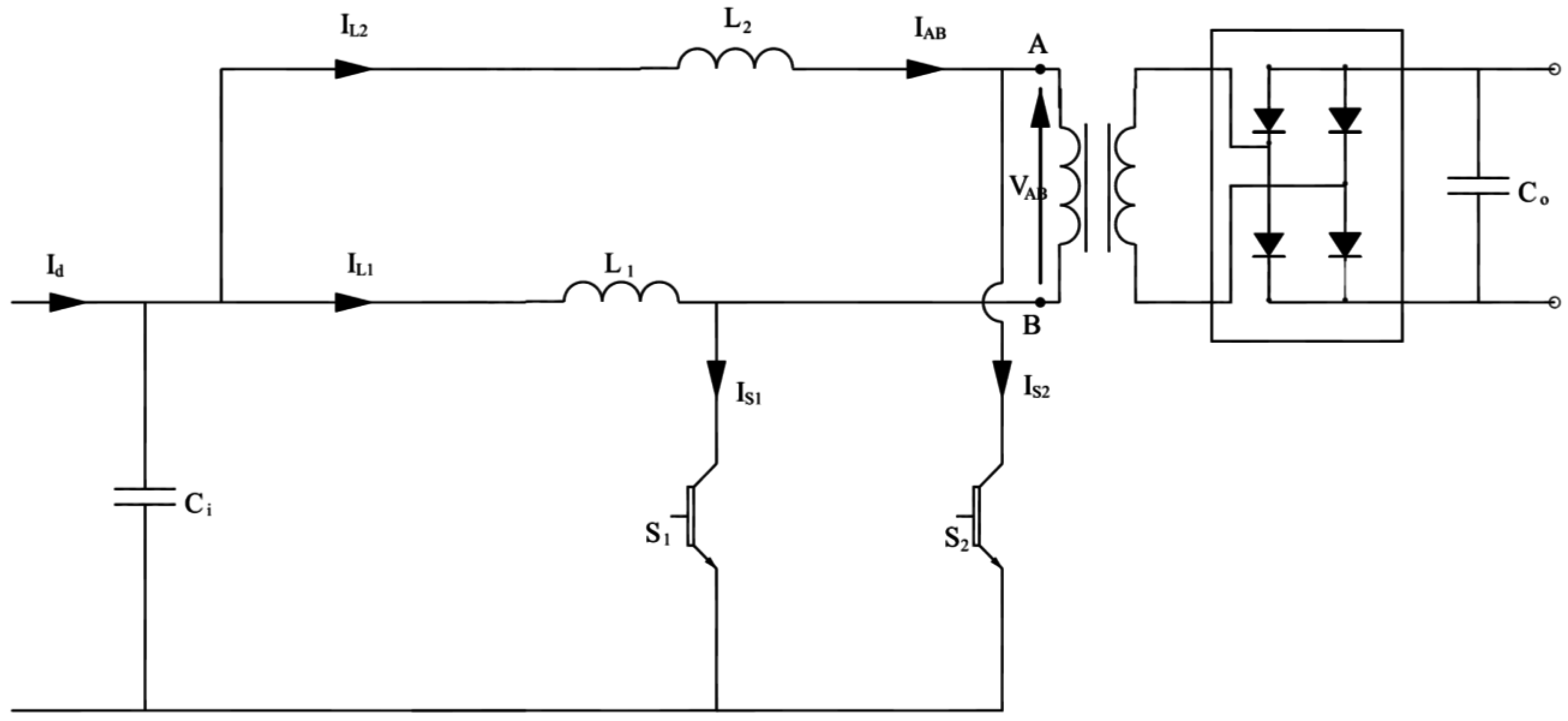
2. Dual Inductor Push-Pull Converter

The basic configuration of a DIIPPC [24] is illustrated in Figure 1. DIIPPCs operate similarly to converters with a single inductor.

Figure 1. Circuit diagram of the dual input inductor push-pull converter.

Figure 1. Circuit diagram of the dual input inductor push-pull converter.

The switches of the input stage are both turned on to charge the input inductors and are alternately turned off to transfer the energy to the primary winding of transformer. The two components are driven with the same control signal delayed by one half of the period. Therefore, a duty cycle greater than 0.5 is sufficient to guarantee the operating principle just described.

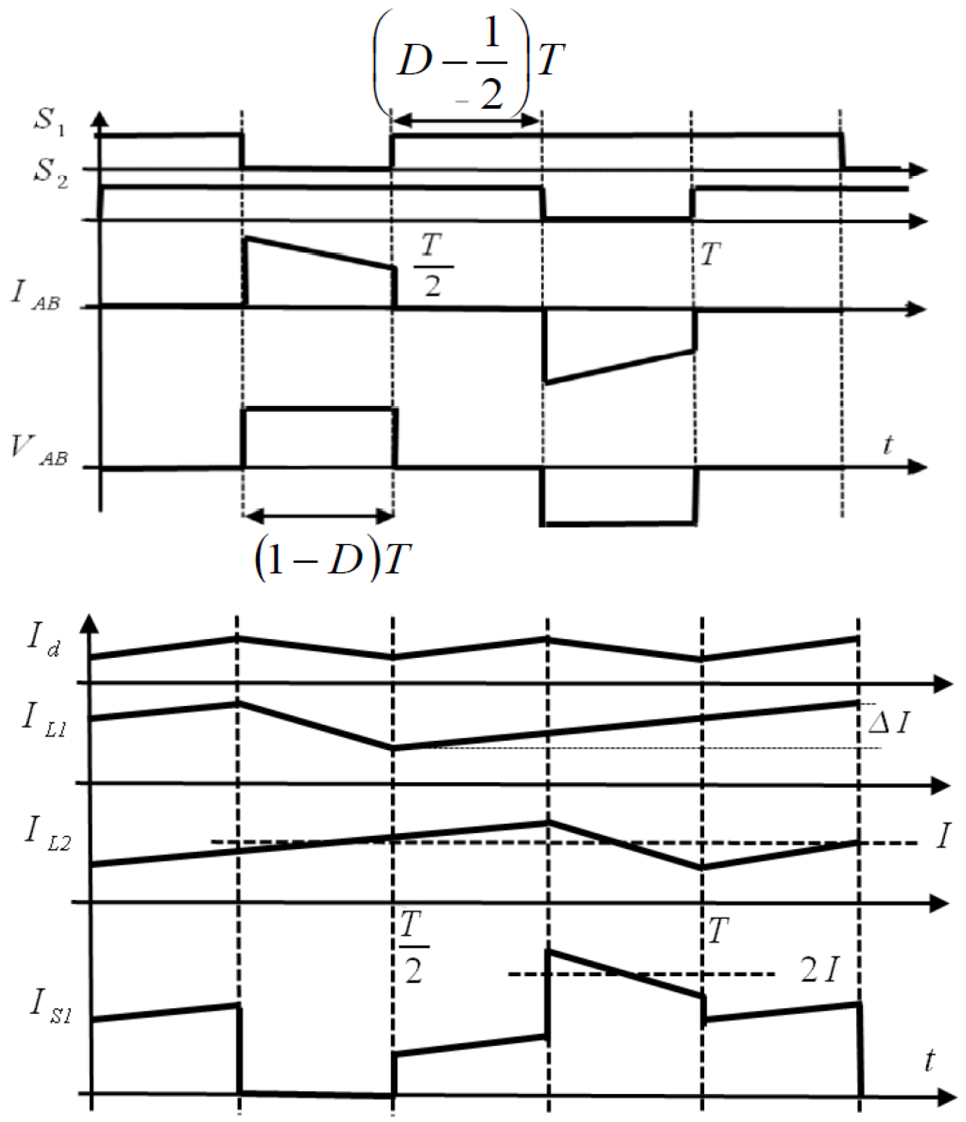
Figure 2 shows the control signals for the switches S1 and S2, the current and the voltage across the transformer, the source current, input inductance currents and the current across one of the main switches for a typical operating condition. In order to make the converter suitable to be used for interfacing PV panels, according with [25,26] an input capacitor is connected. In the hypothesis that this capacitance is high enough, during one switching period the input voltage can be considered constant.

Figure 2. Control signals and primary current and voltage across the transformer (upper diagram); source current, inductor currents and current across the first switch (lower diagram).

Figure 2. Control signals and primary current and voltage across the transformer (upper diagram); source current, inductor currents and current across the first switch (lower diagram).

The output voltage of this converter is increasing with the duty cycle of the switches, because the input stage acts as a boost converter. The output voltage of the converter can be expressed as:

$$V_0=\frac{N_2}{N_1}\frac{V_i}{1-D}$$

(1)

where V_i is the input voltage, D is the duty cycle (defined as the ratio between the on-state time and the switching period, T_on/T), and N₁ and N₂ are the numbers of turns of the primary and secondary windings, respectively.

The rapid change of the inductor current, due to the turn-off of the switch, causes an overvoltage across the switch itself. For this reason, a snubber circuit may be added to reduce the overvoltage. Since the efficiency of the converter is not the main focus of the paper, a traditional dissipative snubber has been used.

3. Adaptive Perturbation Function for P&O Algorithm

The MPPT algorithm proposed by the authors in [10] is a variation of the classic P&O method and has been set up and implemented for the control of the DIIPPC. The main limitation of the P&O algorithm is the compromise between a fast dynamic response and a reduced oscillation at steady-state. Large perturbation steps imply a fast dynamic performance, whereas small perturbation steps ensure little oscillations at steady-state. In particular conditions, during cloudy days, the solar irradiation can vary many times and quickly. This situation can cause fault or reduction of efficiency in MPP trackers. In order to address this problem some studies has been proposed in the technical literature [27,28]. In these conditions, it is necessary to achieve a good dynamic response to avoid losing a great quantity of energy. The efficiency of the P&O technique depends on the perturbation step. It is particularly difficult to find the optimal perturbation step, because this depends on the panel characteristics, working conditions and the converter’s topology. To obtain a faster dynamic with small oscillations without knowing accurately the technical details of the PV system, the proposed adaptive P&O method operates with variable perturbation step adapted to the actual operating conditions. In particular, when the operating point is far from the MPP, large perturbation steps are chosen, whereas small ones are used in proximity to the maximum. Therefore, the algorithm needs to know the MPP position. However, a precise knowledge is not required because the P&O technique always works around the real maximum. In the proposed method, the perturbation step is defined by the following equation:

$$\mathrm{\Delta }V\left(V\right)=f\left(V_{\mathrm{M},\mathrm{est}}-V\right)+\mathrm{\Delta }{V}_{\min }$$

(2)

where ΔV is the perturbation step; V_M,est is the estimated voltage at MPP; V is the measured voltage; ΔV_min is the minimum value of the perturbation.

In order to guarantee a high dynamic performance and limited steady-state oscillations, the function f must be a positive function and must assume a high value when the working point is far from the maximum; moreover, it must be nearly zero in proximity to the maximum. The condition of working in proximity to the MPP is assured by setting ΔV_min at an appropriate value. If the working point is near to the value of V_M,est, ΔV ≈ ΔV_min; when V ≡ V_M,est, f(0) = 0 → ΔV(0) = ΔV_min.

In the previous work [10], f(V_M,est – V) has been chosen to be a quadratic function in the left side of the MPP, and zero in the right side of MPP for stability problems. This procedure for choosing the function given by Equation (2) has not been fully justified and no correlation between f(V_M,est − V) and ΔV_min has been considered. In this paper a criterion to properly choose the adaptive perturbation function is discussed taking into account the possible correlation between the two addends of Equation (2) and the estimation error in evaluating the MPP.

If the MPP voltage estimation were perfect (V_M,est ≡ V_M, where V_M is the actual position of the MPP), and the converter did not introduce delays, the best expression for f and ΔV_min would be:

$$\begin{array}{l}f\left(V_{\mathrm{M},\mathrm{est}}-V\right)=\left|V_{\mathrm{M},\mathrm{est}}-V\right|\\ \mathrm{\Delta }{V}_{\min }=0\end{array}$$

(3)

In this ideal condition, the MPP would be reached after one iteration. However, the MPP voltage estimation introduces an error. Therefore, in order to make the algorithm capable of reaching the actual MPP, it is necessary to have ΔV_min ≠ 0. In addition, when the measured voltage V is close to V_M, the function f should yield a value lower than ΔV_min when V ≡ V_M:

$$f\left(V_{\mathrm{M},\mathrm{est}}-V_{\mathrm{M}}\right)<\mathrm{\Delta }{V}_{\min }$$

(4)

The condition given by Equation (4) guarantees that f helps to increase the rapidity of the MPPT algorithm far from the maximum power point, but does not worsen the oscillations when the PV array is operating around V_M. Indicating with k the maximum estimation error in p.u. it is:

$$\frac{\left|V_{\mathrm{M},\mathrm{est}}-V_{\mathrm{M}}\right|}{V_{\mathrm{M}}}\le k$$

(5)

The algorithm has to be capable of correctly matching the MPP also in case of wrong estimation of V_M. For this reason, a minimum perturbation step has to be introduced, as reported in Equation (2). Being k the maximum allowed estimation error, the algorithm could go to work in a point far from the real MPP of, at worst, kV_M. In order to achieve the correct matching of the MPP it has to be:

$$\mathrm{\Delta }{V}_{\min }>k{V}_{\mathrm{M}}$$

(6)

In this way, the P&O action can compensate the estimation error in two steps.

Equation (6) proves that the linear expression (3) cannot be used in practice because estimation errors would be too high to ensure small oscillations at steady state. For this reason, polynomial expressions with higher order or exponential expressions are preferred in the practical implementation of the algorithm. Choosing, for example, a quadratic function:

$$f\left(V_{\mathrm{M},\mathrm{est}}-V\right)=a\hspace{0.17em}{\left(V_{\mathrm{M},\mathrm{est}}-V\right)}^2$$

(7)

It is possible to set a high value for f in order to have a quick answer when the voltage is far from the MPP. In particular, when V is zero (the furthest position), the MPP can be reached in two steps if the function f is selected as:

$$f\left(V_{\mathrm{M},\mathrm{est}}\right)=0.5\hspace{0.17em}{V}_{\mathrm{M},\mathrm{est}}$$

(8)

This last equation, together with Equation (7), gives the value of parameter a:

$$a=\frac{0.5}{V_{\mathrm{M},\mathrm{est}}}$$

(9)

Substituting the expression of f (given by Equation (7)) into Equation (4), and using Equation (9) for parameter a, it is possible to obtain the following condition on ΔV_min:

$$\mathrm{\Delta }{V}_{\min }>\frac{0.5}{V_{\mathrm{M},\mathrm{est}}}\hspace{0.17em}{\left(V_{\mathrm{M},\mathrm{est}}-V_{\mathrm{M}}\right)}^2=A$$

(10)

where the quantity A systemizes the right term of the inequality. Moreover, from Equation (5) the following condition can be obtained:

$$A=\frac{0.5}{V_{\mathrm{M},\mathrm{est}}}{\left(V_{\mathrm{M},\mathrm{est}}-V_{\mathrm{M}}\right)}^2\le \frac{0.5}{V_{\mathrm{M},\mathrm{est}}}{V_{\mathrm{M}}}^2{k}^2=B$$

(11)

where the quantity B synthesizes the right term of the inequality. In order to satisfy condition (10) it is possible to choose ΔV_min higher than B, i.e., if ΔV_min >B ⇒ ΔV_min >A (since A ≤ B):

$$\mathrm{\Delta }{V}_{\min }>B\hspace{1em}\hspace{1em}\Rightarrow \hspace{1em}\hspace{1em}\{\begin{array}{l}\mathrm{\Delta }{V}_{\min }>A\\ \mathrm{with:}\hspace{0.17em}A\le B\end{array}\hspace{1em}\hspace{1em}$$

(12)

Thus, ΔV_min > B is a sufficient (but not necessary) condition to satisfy Equation (10). Solving Equation (5) it is possible to deduce the following conditions on V_M,est, and, consequently on the quantity B:

$$\frac{\left|V_{\mathrm{M},\mathrm{est}}-V_{\mathrm{M}}\right|}{V_{\mathrm{M}}}\le k\hspace{1em}\Rightarrow \hspace{1em}\{\begin{array}{l}{V}_{\mathrm{M},\mathrm{est}}\in \left]V_{\mathrm{M}},\hspace{0.17em}\left(1+k\right)V_{\mathrm{M}}\right]\\ \hspace{0.17em}\hspace{0.17em}\hspace{0.17em}\hspace{0.17em}\hspace{0.17em}\hspace{0.17em}\hspace{0.17em}\hspace{0.17em}\hspace{0.17em}\hspace{0.17em}\hspace{0.17em}\hspace{0.17em}\hspace{0.17em}\hspace{0.17em}\hspace{0.17em}\hspace{0.17em}\hspace{0.17em}\hspace{0.17em}\hspace{0.17em}\hspace{0.17em}\mathrm{or}\\ V_{\mathrm{M},\mathrm{est}}\in \left[\left(1-k\right)V_{\mathrm{M}},\hspace{0.17em}{V}_{\mathrm{M}}\right[\end{array}\hspace{1em}\Rightarrow \hspace{1em}{V}_{\mathrm{M},\mathrm{est}}\ge \left(1-k\right)V_{\mathrm{M}}\hspace{1em}\iff \hspace{1em}B\le \frac{0.5\hspace{0.17em}{k}^2}{\left(1-k\right)}{V}_{\mathrm{M}}=C$$

(13)

where the quantity C synthesizes the right term of the last inequality. In order to satisfy ΔV_min > B it is possible to choose ΔV_min higher than C, i.e., if ΔV_min > C ⇒ ΔV_min > B (since B ≤ C):

$$\mathrm{\Delta }{V}_{\min }>C\hspace{1em}\hspace{1em}\Rightarrow \hspace{1em}\hspace{1em}\{\begin{array}{l}\mathrm{\Delta }{V}_{\min }>B\\ \mathrm{with:}\hspace{0.17em}B\le C\end{array}$$

(14)

which, substituting the expression of the term C, gives:

$$\mathrm{\Delta }{V}_{\min }>0.5\hspace{0.17em}\frac{k^2}{\left(1-k\right)}{V}_{\mathrm{M}}$$

(15)

Equation (15) returns a minimum variable step of 0.56% for a 10% estimation error, which ensures reasonably small oscillations at steady state.

4. PV Panel Identification

The PV array is composed of 36 cells of monocrystalline silicon wafers, connected in series and measuring a total active area of 0.54 m². The technical data of the PV array are reported in Table 1. The PV array model is mathematically described by the following equations [10]:

$$\begin{array}{l}V=\frac{AKT}{q}\ln \left(\frac{I-I_{\mathrm{ph}}-I_{\mathrm{sat}}}{I_{\mathrm{sat}}}\right)-r_{\mathrm{s}}I\\ I_{\mathrm{ph}}=\left[I_{\mathrm{scr}}+k_i\left(T-T_{\mathrm{r}}\right)\right]\hspace{0.17em}s\\ I_{\mathrm{sat}}=I_{\mathrm{rr}}{\left(\frac{T}{T_{\mathrm{r}}}\right)}^3\exp \left[\frac{q\hspace{0.17em}{E}_{\mathrm{g}}}{K}\left(\frac{1}{T_{\mathrm{r}}}-\frac{1}{T}\right)\right]\end{array}$$

(16)

where I_scr is the short circuit current, I_rr is the reverse current at the reference temperature, q is the electronic charge, A is the junction ideality factor, K is the Boltzmann constant, T is the absolute temperature of the array, T_r is a constant equal to 273.14 K, r_s is the series resistance, s is the p.u. irradiation, E_g is the band gap energy of the semiconductor, and k_i is the short-circuit current temperature coefficient.

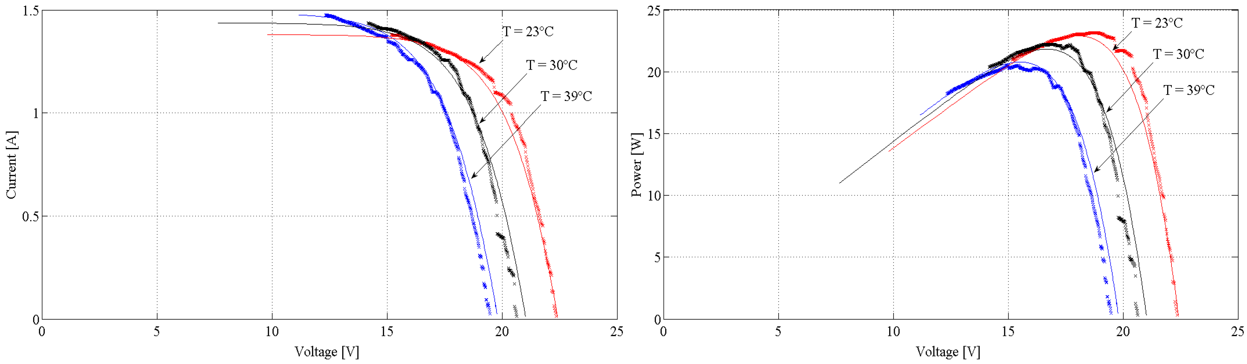
The curves of the PV array have been evaluated experimentally for several temperatures, ranging from 23 °C to 40 °C with a step of 1 °C. However, only some of these curves are presented in Figure 3 for a better visualisation. The tests were made with an artificial light to control the level of irradiance and keep the irradiance smooth during the test. The open circuit voltage of the panel, V_oc, presents a decreasing rate of 2.3 mV/°C, whereas the short-circuit current, I_scr, presents an increasing rate of 0.2%/°C. This is reflected by a power peak reduction, which is equal to 0.6%/°C–0.7%/°C. The experimental data have been fitted using a least mean square numeric procedure in order to obtain the parameters of the model. The results of this procedure are shown in Table 2. The curves obtained by the model are also plotted in Figure 3, showing very good agreement with the experimental data.

Table 1. Characteristics of PV array.

Type	Aluminum-Tedlar125M36
Open circuit voltage, Voc	21.85 V
Short circuit current, Isc	4.52 A
Maximum power, PM	69.03 W
Maximum power voltage, VM	17.74 V
Maximum power current, IM	3.89 A

Table 1. Characteristics of PV array.

Type	Aluminum-Tedlar125M36
Open circuit voltage, Voc	21.85 V
Short circuit current, Isc	4.52 A
Maximum power, PM	69.03 W
Maximum power voltage, VM	17.74 V
Maximum power current, IM	3.89 A

Table 2. Main data of the PV panel used.

A [–]	Irr [nA]	rs [Ω]	Iscr [A]	ki [A/K]
57	−15.8	0.25	3.5	0.001

Table 2. Main data of the PV panel used.

A [–]	Irr [nA]	rs [Ω]	Iscr [A]	ki [A/K]
57	−15.8	0.25	3.5	0.001

Figure 3. PV current and power curves for different array temperatures and their fitting.

Figure 3. PV current and power curves for different array temperatures and their fitting.

5. Algorithm Implementation

The MPPT algorithm presented in this paper requires the estimation of the maximum V_M. Once the panel has been identified according to the procedure of the previous section, the theoretical position of V_M can be determined by the mathematical model of the panel. In practical applications the characteristic of the panel changes during its life for ageing and dust. For this reason, a periodical characterization has to be performed and the experimental characteristic has to be registered. A good time interval for characterization of the panel can be one month. During one month the efficiency degradation of a PV panel has been estimated to be 7% [29]. Anyway, with the proposed algorithm, an error in the estimation of the theoretical maximum is compensated by the P&O function. As analyzed in Section 7 a 10% error in the estimation of V_M does not practically affect the performances of the proposed algorithm. It is worth noting that, the chosen converter, allows the complete catching of panel characteristic because it can make the panel work from short circuit (duty cycle equal to 1) to open circuit (duty cycle equal to 0).

In order to estimate the MPP voltage and current, it is necessary to measure the irradiation and the temperature. Although it is quite easy and inexpensive to measure the temperature, the measurement of the irradiation greatly increases the cost of the MPPT control system. For this reason, the power-voltage characteristic has been preferred to the power-current characteristic. Indeed, the voltage at the MPP is weakly variable with the irradiation, whereas the current at the MPP is weakly variable with the temperature. In the following figures, the irradiation is normalised to 1 kW/m². Figure 4 shows the MPP voltage as a function of the irradiation for different temperatures.

Figure 4. MPP voltage vs. irradiation for different temperatures.

Figure 4. MPP voltage vs. irradiation for different temperatures.

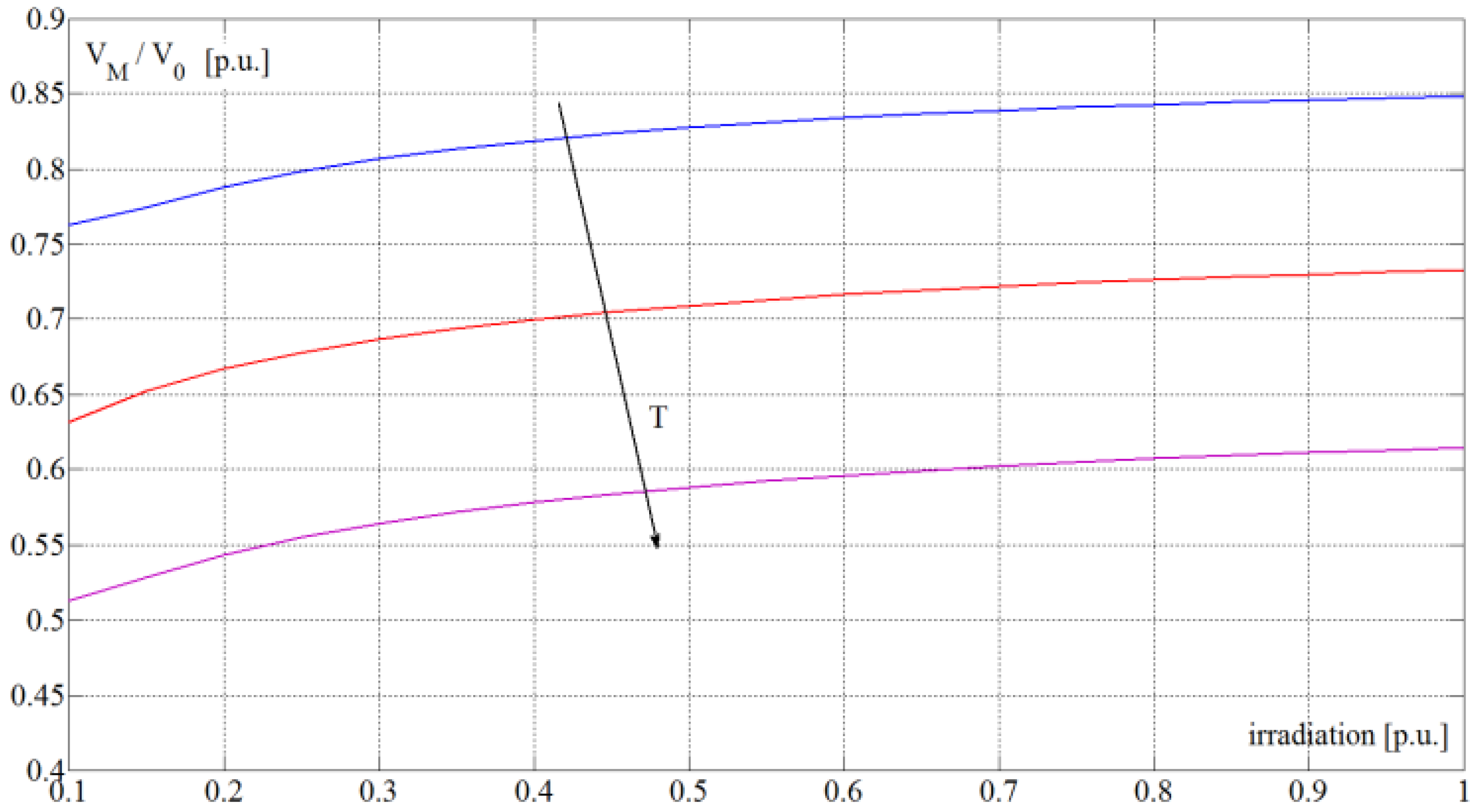
The power-voltage characteristic has been chosen for the algorithm implementation, in order to use only one temperature sensor for the individuation of the maximum position. Using the parameters of the panel, reported in Table 2, the error committed in the MPP voltage estimation is reported in Figure 5.

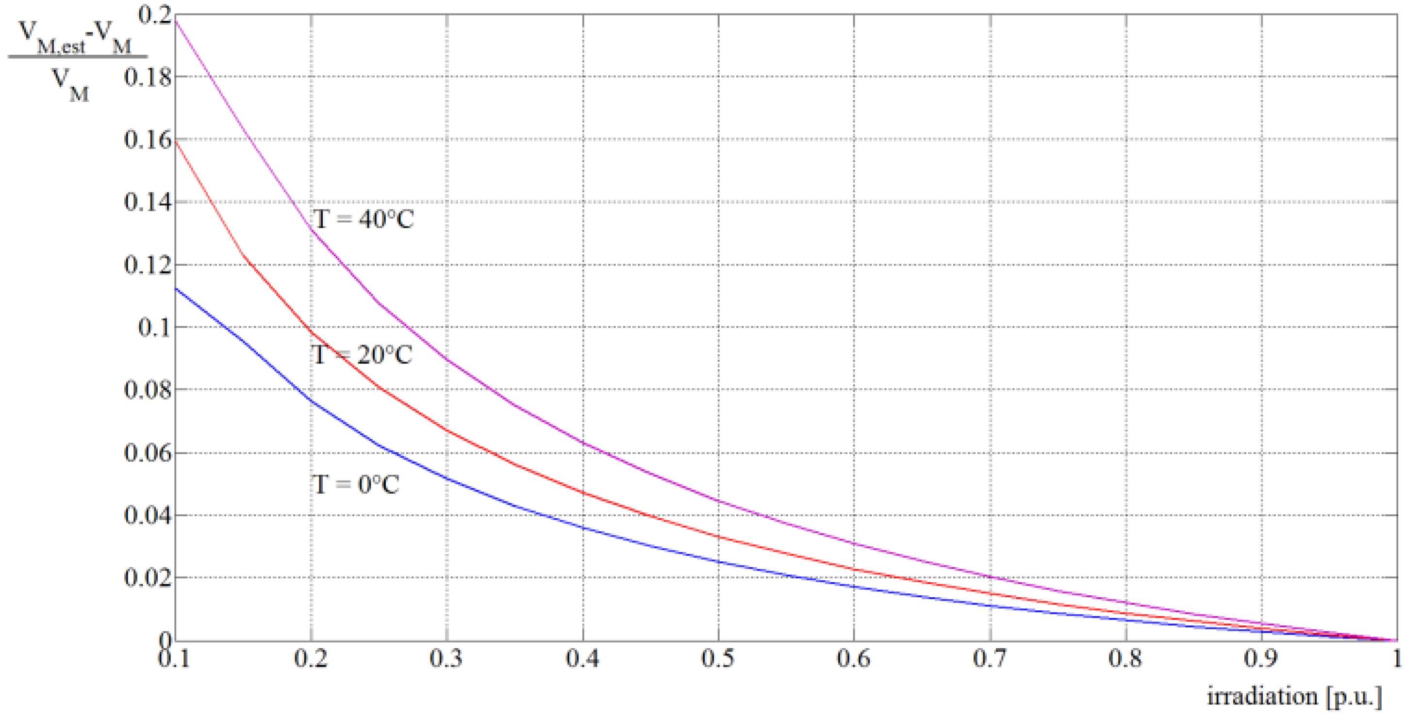
Figure 5. MPP voltage estimation error in p.u. vs. irradiation for different temperatures.

Figure 5. MPP voltage estimation error in p.u. vs. irradiation for different temperatures.

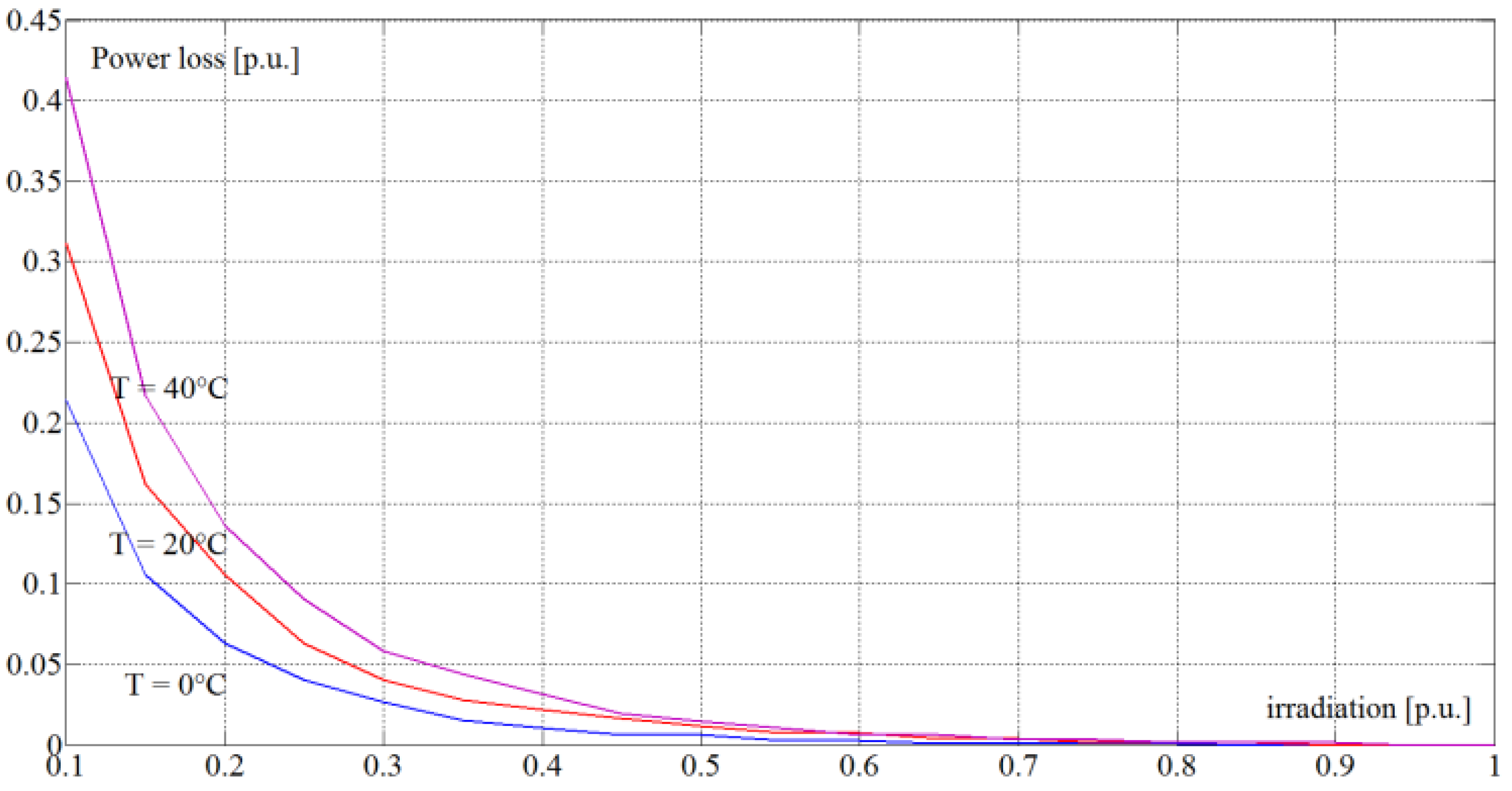
Figure 5 shows that when the irradiation is higher than 0.3 p.u. the MPP voltage estimation error is lower than 10%. Without a P&O algorithm, a MPP voltage estimation error implies a power loss with respect to the maximum power that can be generated. Figure 6 shows this power loss in per unit of the nominal array power as a function of the p.u. irradiation for different temperatures.

Figure 6. Power loss in p.u. vs. irradiation for different temperatures.

Figure 6. Power loss in p.u. vs. irradiation for different temperatures.

If the irradiation is higher than 0.3 p.u., the power losses are lower than 10% over a wide temperature variation range. Thus, the proposed algorithm has efficiency higher than 90% during quick transients. This error is reduced by the P&O action and is very low at a steady-state for a low value of ΔV_min.

6. Test Bench and Experimental Results

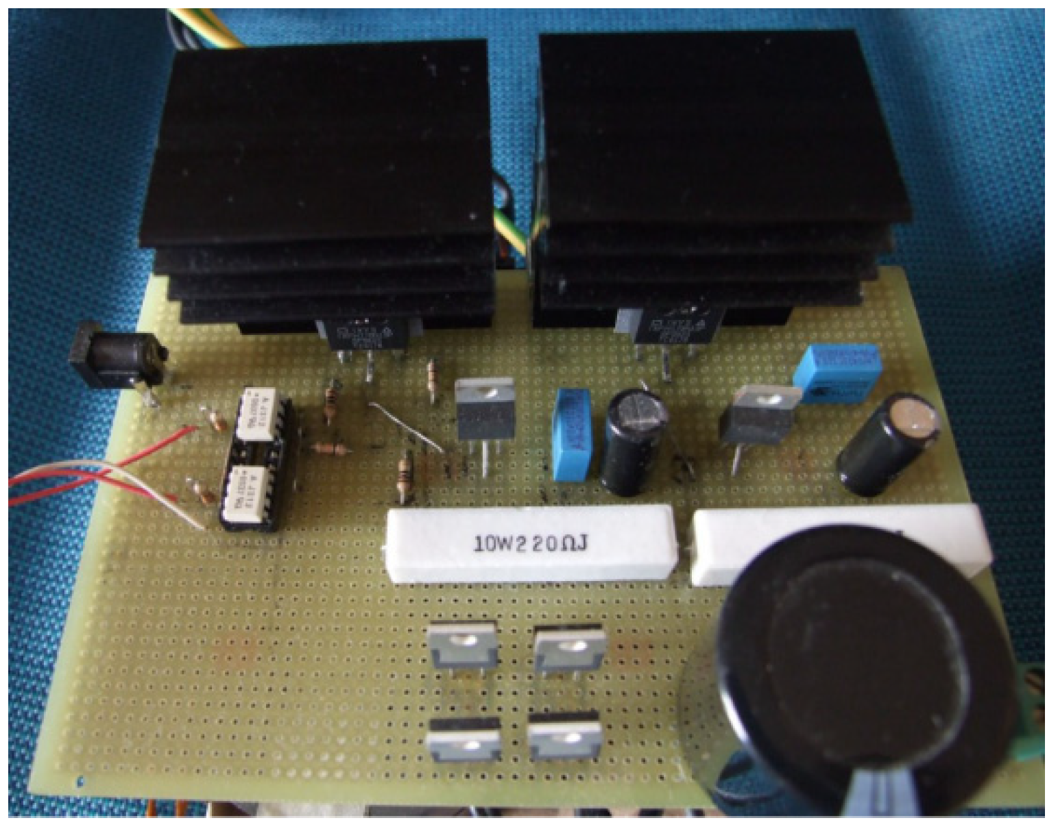
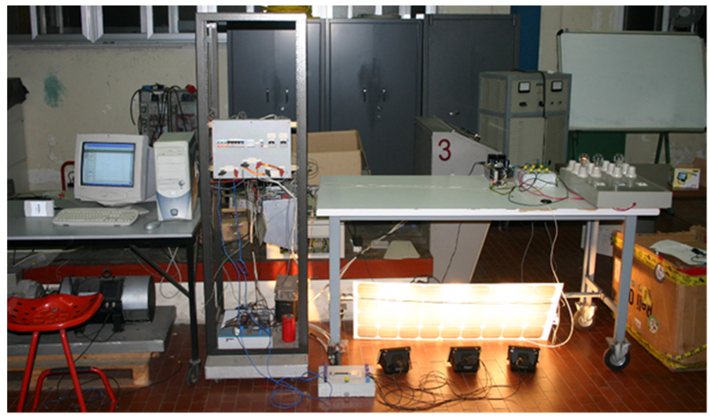
The MPPT technique proposed in this paper has been experimentally tested on a laboratory prototype of a PV system, shown in Figure 7. Figure 8 and Figure 9 show also a close-up view of the DIIPPC used for experiments. The test bench permits the simulation of different operating conditions of solar irradiations and temperatures.

Figure 7. Photograph of the test bench used for the experimentation.

Figure 7. Photograph of the test bench used for the experimentation.

The ratings of the DIIPPC are reported in Table 3. The ripple of the current is below 1 A under rated conditions. Snubber circuits, with capacitance and resistance of 47 μF and 220 Ω, respectively, are used to protect the power Mosfets 170N10P, manufactured by IXYS (Milpitas, CA, USA). These switches have a nominal voltage of 100 V and a nominal current of 170 A. The capacitance value has been selected to store an amount of energy double than that stored in one input inductor under rated conditions. The resistance was selected on the basis of the energy discharged by the snubber capacitor at the rated voltage.

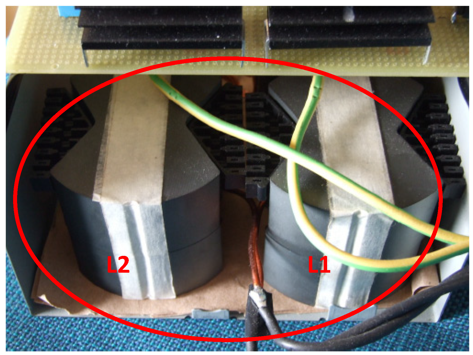
Figure 8. Close-up front view of the DIIPPC.

Figure 8. Close-up front view of the DIIPPC.

Table 3. Characteristics of the DC-DC converter.

Rated Power	Rated Input Voltage	Rated Output Voltage	Switching Frequency	Input Current Ripple	Drain to Source Mosfet Voltage	Inductances Value	Transformer Ratio
300 W	10 V	100 V	100 kHz	<3%	100 V	80 μH	4:12

Table 3. Characteristics of the DC-DC converter.

Rated Power	Rated Input Voltage	Rated Output Voltage	Switching Frequency	Input Current Ripple	Drain to Source Mosfet Voltage	Inductances Value	Transformer Ratio
300 W	10 V	100 V	100 kHz	<3%	100 V	80 μH	4:12

The control of the converter is based on the PIC 18F4550 microcontroller by Microchip (Chandler, AZ, USA), which features a PWM module for the gate drivers of the switches. The microcontroller inputs are the array temperature measured by a thermocouple, the PV voltage and the PV current. The thermocouple is placed on the back of the PV array, whereas the current is measured using a shunt resistor.

Figure 9. Close-up rear view of the DIIPPC.

Figure 9. Close-up rear view of the DIIPPC.

The solar irradiation has been simulated by means of three halogen lamps, each one having a power of 500 W. Different solar conditions are simulated regulating the power irradiated by the lamps. The use of halogen lamps is not ideal for testing PV systems. Anyway, the use of artificial light is the only method for ensuring the same variable conditions for testing different MPPT algorithms. Moreover, being the same the irradiation change, also if it is not the ideal light for optimizing the panels, the results, in terms of comparison between different MPPTs can be considered correct. That’s why, also in [30] the authors use halogen lamps for simulating controllable irradiation conditions.

In order to evidence the differences between the different algorithms, some step changes in the solar irradiation have been simulated. Also if this condition is not so frequent, in nature, the step change in solar irradiation represents a good test for comparing the dynamic response of different MPPT algorithms [27].

A 100 Ω resistor has been used as a load. The actual load seen by PV array is dependent on the duty-cycle of the converter according to the following relationship:

$$R_{\mathrm{actual}}=R_{\mathrm{load}}\frac{{\left(1-D\right)}^2{N}_1^2}{N_2^2}$$

(17)

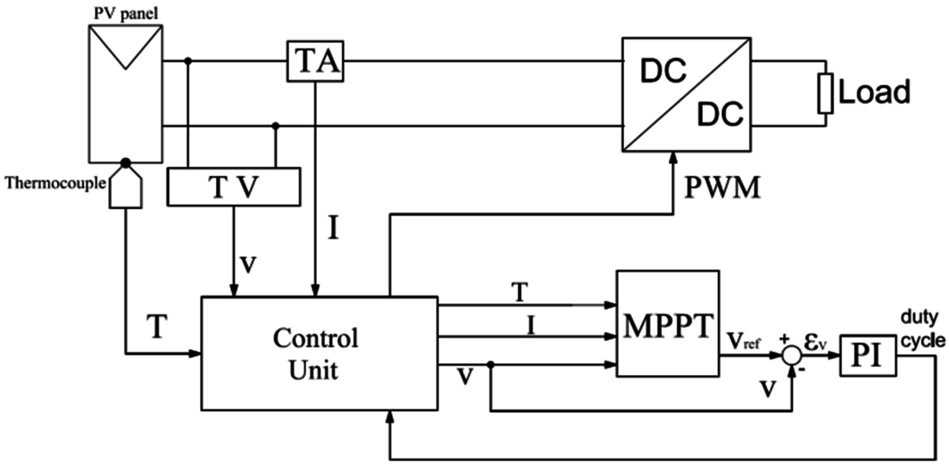
A block diagram of the system control is represented in Figure 10. The MPPT algorithm is implemented by changing the duty-cycle of the DIIPPC via a proportional-integral regulator. The constants of the regulator have been selected in order to obtain a good compromise between good dynamic of MPPT and reduced steady-state oscillations around the MPP. After several tests, have been chosen the values: k_p = −0.03 and k_i = 1.5. The two constants are negative because, for the electrical characteristic of the PV source, an increasing duty cycle of the converter implies a reduction of the output voltage of the PV system.

Figure 10. Block diagram of the control system.

Figure 10. Block diagram of the control system.

The modified P&O algorithm proposed in this paper has been experimentally compared to a traditional P&O. In order to enhance the performances of the traditional P&O, some preliminary tests were carried out in order to find the best perturbation step, i.e. the step capable of extracting the maximum average power from the PV panel. To this aim, a sample irradiation pattern was created, consisting of 30 s of full irradiation, 30 s of 40% irradiation, and another 30 s of full irradiation. At a temperature of 23 °C, the best step for the traditional P&O is 0.3 V, whereas at 32 °C it is 0.7 V.

The performances of the modified P&O algorithm are strongly dependent on the function f, which defines the adaptive step of the algorithm. Experimental tests showed that the best results are obtained when f is a quadratic polynomial function, with a minimum perturbation step of 0.05 V at the maximum power point voltage under rated conditions. This result is in accordance with the consideration reported in Section 3.

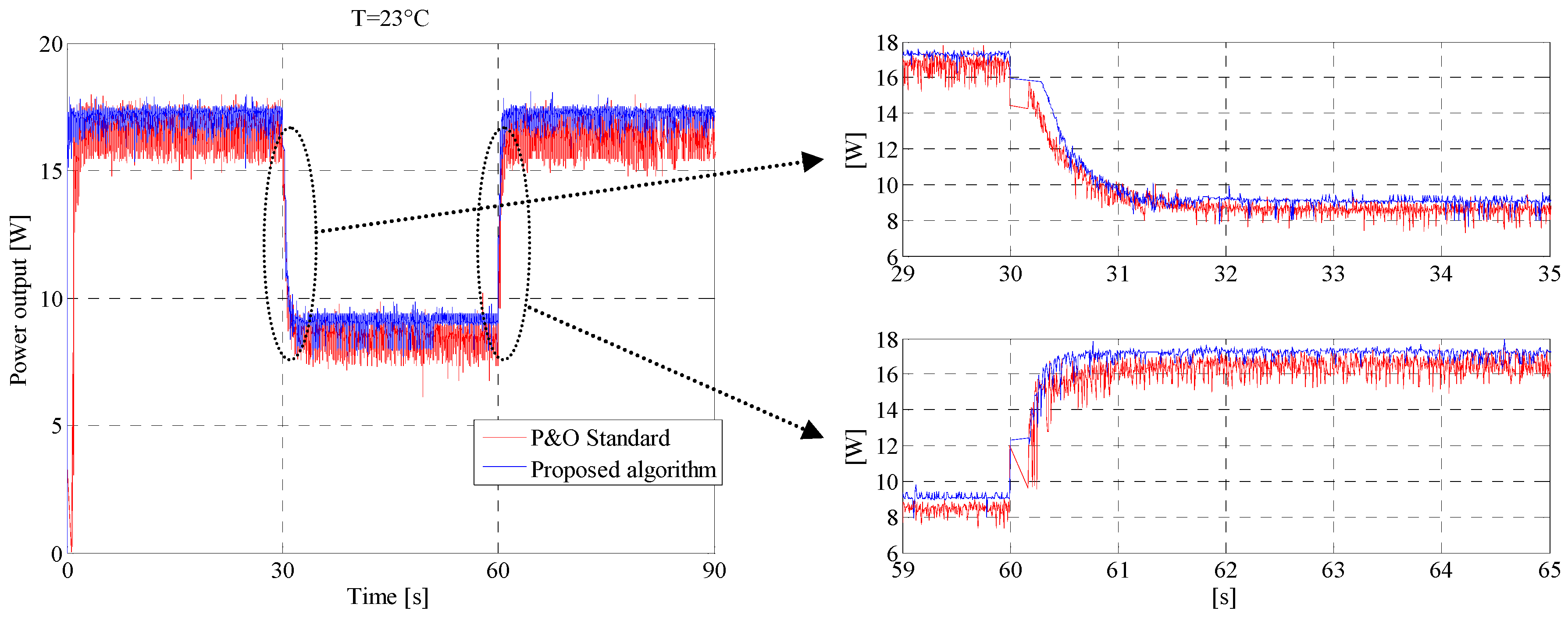
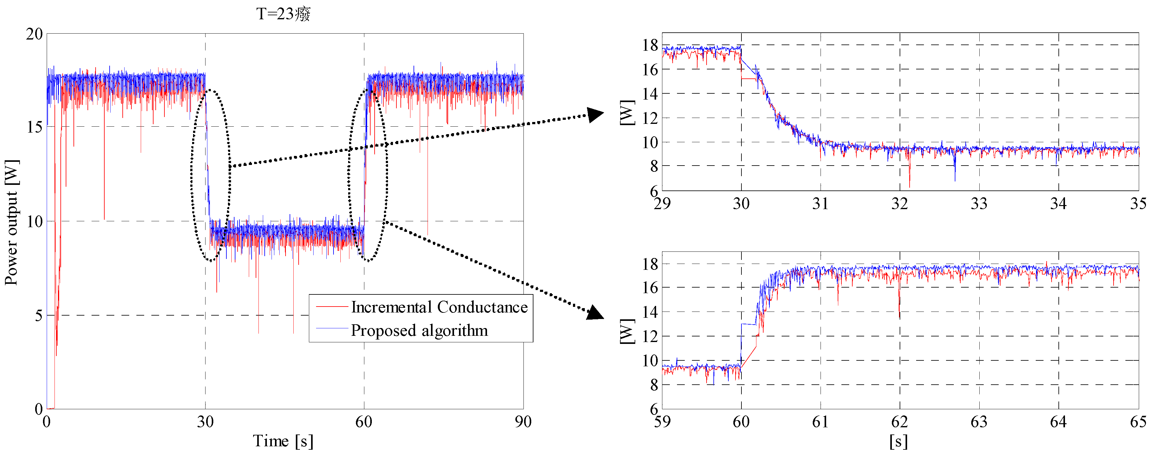
The results of the comparison are presented in Figure 11 for a temperature of 23 °C. The left side of Figure 11 clearly shows that the proposed modified P&O algorithm is better than the standard P&O at steady-state, because the oscillations are smaller and the average power level is higher. During transients (starting at t = 30 s and t = 60 s) the proposed method shows the same reactivity of the standard P&O, as shown in the right side of Figure 11.

Figure 11. Comparison between the proposed algorithm and a standard P&O at 23 °C.

Figure 11. Comparison between the proposed algorithm and a standard P&O at 23 °C.

This means that the enhanced oscillations around the maximum of the proposed method is not paid with a slower dynamic capability, as it would happen for a traditional P&O algorithm. Indeed the perturbation step is higher when the irradiation changes suddenly and is lower when the operating point is close to the maximum power point. Moreover, the good performance at steady-state is also guaranteed by the smooth variation of the perturbation step, which is obtained by the quadratic shape of the function f. 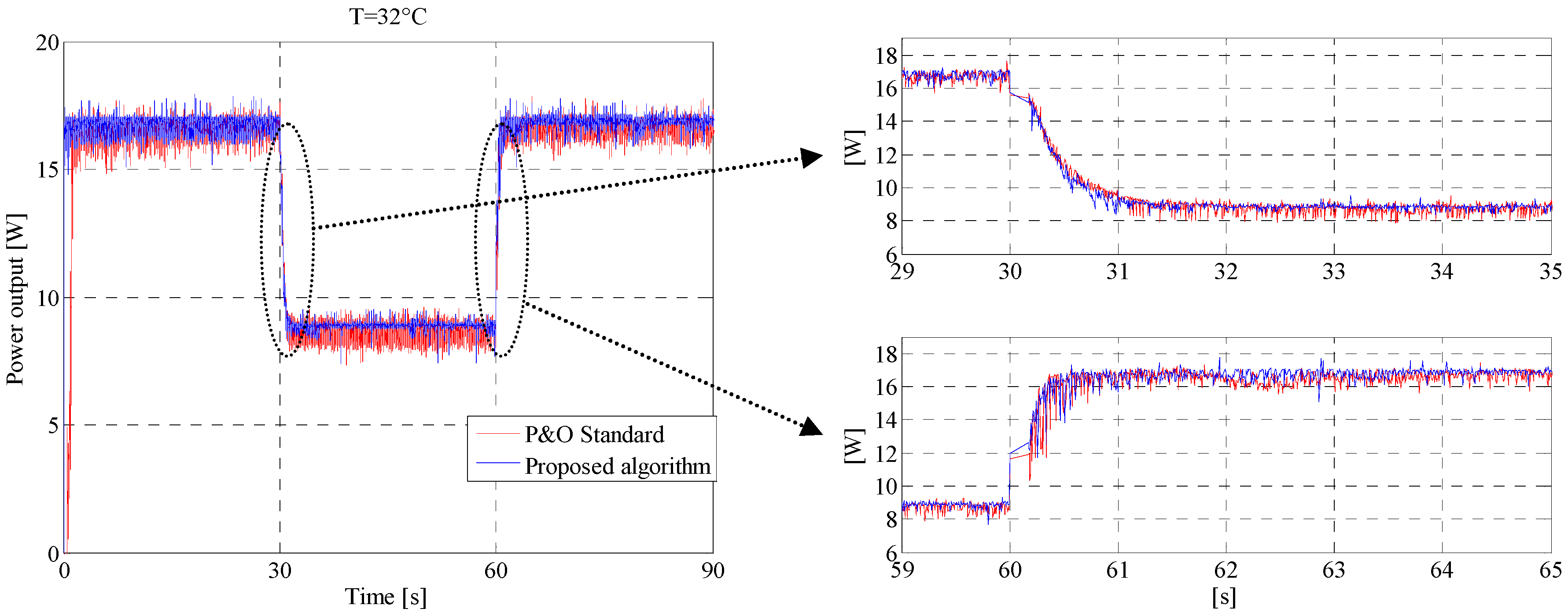Figure 12 shows a similar behaviour for a temperature of 32 °C.

Figure 12. Comparison between the proposed algorithm and a standard P&O at 32 °C.

Figure 12. Comparison between the proposed algorithm and a standard P&O at 32 °C.

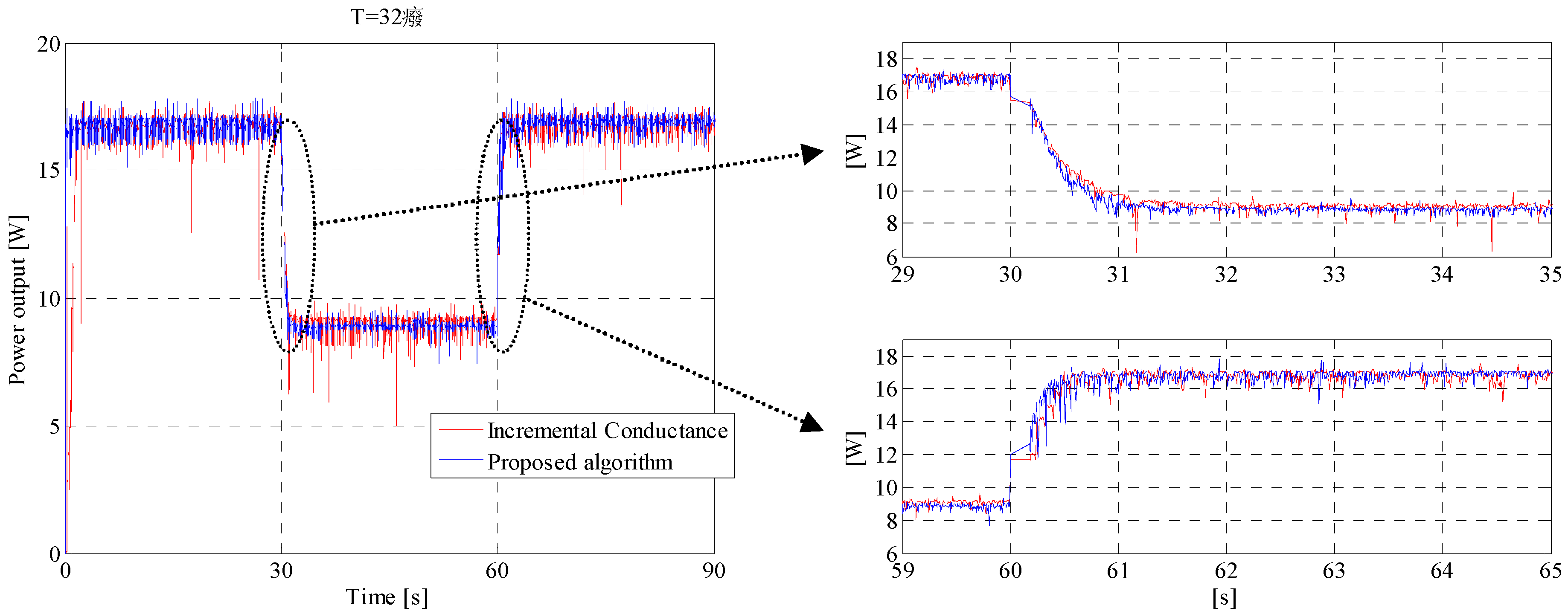
It is important to notice that at 32 °C the perturbation voltage step for the traditional P&O has been changed from 0.3 to 0.7 in order to assure the maximum average power and a good dynamic; this adjustment was not necessary for the proposed modified P&O technique, which shows the same reactivity for different temperatures. The proposed MPPT algorithm has also been compared to the IC algorithm. As for the case of the traditional P&O, the IC algorithm was tuned in order to define the best perturbation step. The comparison between the proposed algorithm and IC algorithm is reported in Figure 13 for a temperature of 23 °C.

Figure 13. Comparison between the proposed algorithm and IC method at 23 °C.

Figure 13. Comparison between the proposed algorithm and IC method at 23 °C.

The diagrams show that situation is similar to that of Figure 11, where the proposed algorithm shows smaller oscillations and higher average power level together with comparable dynamics during transients. Figure 14 shows that a similar behaviour is observed when the temperature is 32 °C. Finally Table 4 summarizes the average power experimentally obtained from the panel using the three algorithms under the solar irradiations of Figure 10, Figure 11, Figure 12, Figure 13 and Figure 14.

Figure 14. Comparison between the proposed algorithm and IC method at 32 °C.

Figure 14. Comparison between the proposed algorithm and IC method at 32 °C.

Table 4. Average power obtained from different algorithms.

Temperature	Standard P&O	Incremental Conductance	Modified P&O
23 °C	14.1 W	14.1 W	15.0 W
32 °C	14.1 W	14.1 W	14.5 W

Table 4. Average power obtained from different algorithms.

Temperature	Standard P&O	Incremental Conductance	Modified P&O
23 °C	14.1 W	14.1 W	15.0 W
32 °C	14.1 W	14.1 W	14.5 W

As it can be seen from the values of Table 4, the proposed algorithm reaches higher average power in comparison to traditional methods; the increment is 3.6% depending on the operating temperature.

An extensive study was carried out in order to evaluate the conversion efficiencies of the three algorithms considered in this paper. For each operating temperature, the solar irradiation was estimated by the short circuit current, which is directly proportional to the irradiation. For the nominal irradiation of 1000 W/m² and temperature of 25 °C, the short circuit current is about 300 A/m². For different temperatures, the short circuit current has been modified by the factor 0.2%/°C, as explained in Section 4. Therefore, the power reaching the panel is the product of the instantaneous irradiation times the area of the array A_c. If the power output of the panel is indicated as p(t) and the solar irradiation as I(t), the efficiency of the panel, η, can be evaluated as follows:

$$\mathrm{\eta }=\frac{{\displaystyle \underset{0}{\overset{T}{\int }}p\left(t\right)dt}}{A_{\mathrm{c}} {\displaystyle \underset{0}{\overset{T}{\int }}I\left(t\right)\hspace{0.17em}}dt}$$

(18)

Table 5 gives the results of the comparison of the three algorithms for several operating temperatures in terms of panel efficiencies. From the examination of Table 4 and Table 5, it is clear that the modified P&O algorithm proposed in this paper has efficiency higher than that of the algorithms traditionally described in the technical literature. The shape of the smoothing function, which modifies the perturbation step, plays a key role in improving the transitions after a change in the solar irradiation and reduces the steady-state oscillations around the MPP.

Table 5. Panel efficiencies obtained from different algorithms.

Temperature	23 °C	26 °C	28 °C	30 °C	32 °C	35 °C	36 °C	40 °C	44 °C
Standard P&O	8.9%	9.0%	9.2%	9.0%	8.9%	9.0%	9.0%	8.8%	8.4%
Incremental Conductance	9.1%	9.2%	8.8%	9.1%	8.9%	9.0%	9.1%	8.5%	8.5%
Modified P&O	9.5%	9.6%	9.3%	9.3%	9.2%	9.2%	9.2%	8.9%	8.6%

Table 5. Panel efficiencies obtained from different algorithms.

Temperature	23 °C	26 °C	28 °C	30 °C	32 °C	35 °C	36 °C	40 °C	44 °C
Standard P&O	8.9%	9.0%	9.2%	9.0%	8.9%	9.0%	9.0%	8.8%	8.4%
Incremental Conductance	9.1%	9.2%	8.8%	9.1%	8.9%	9.0%	9.1%	8.5%	8.5%
Modified P&O	9.5%	9.6%	9.3%	9.3%	9.2%	9.2%	9.2%	8.9%	8.6%

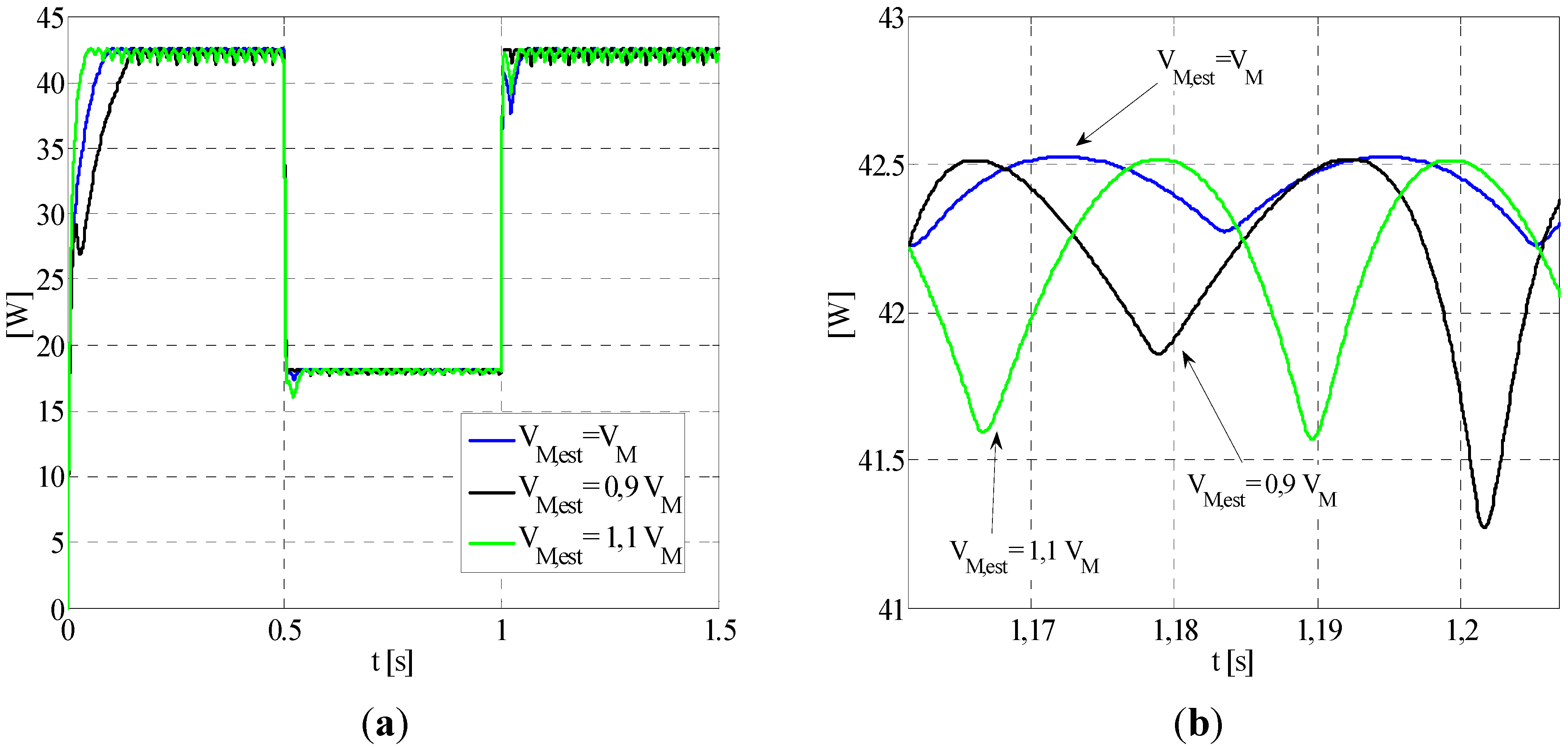
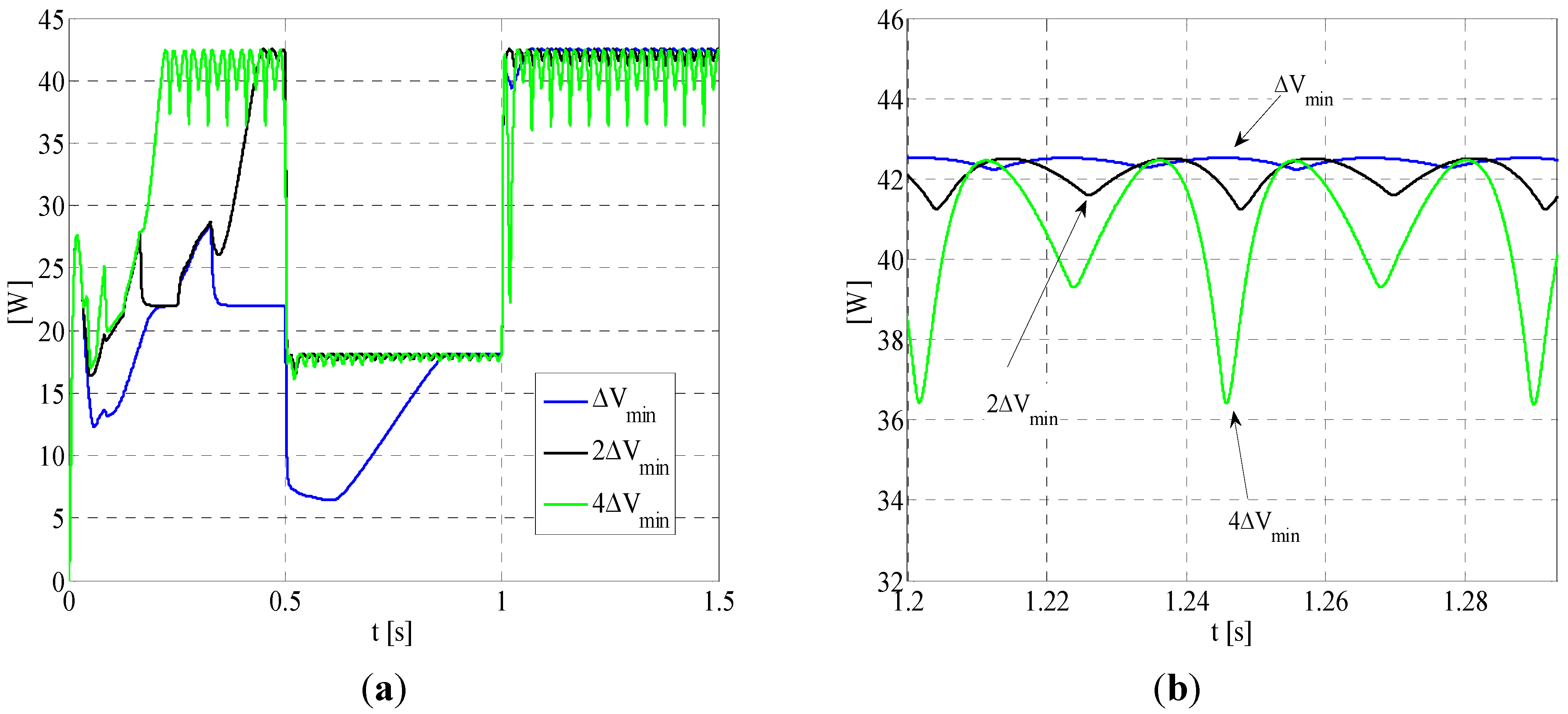
7. Additional Discussion on the MPP Estimator Error

As additional investigations a numerical analysis is carried out supposing that the actual MMP is estimated with a ±10% of error; that produces a ΔV_min according to Equation (15). In these simulations the irradiation starts from value of 1 p.u., at time of 0.5 sec. decrease to 0.45 p.u. and gets back to 1 p.u. at time of 1.0 sec. For the proposed modified P&O algorithm, Figure 15 shows the output power in the cases V_M,est = 0.9 V_M and V_M,est = 1.1 V_M, together with the perfect estimation case V_M,est = V_M. Since the performance of a traditional P&O method is strongly influenced by the voltage perturbation step, several simulations were carried out. In Figure 16 the result of a traditional P&O algorithm with the settings ΔV = ΔV_min, ΔV = 2 ΔV_min and ΔV = 4 ΔV_min, is reported in terms of output power. The simulations shows that, for the irradiation pattern selected, the traditional P&O method is unable to reach the MPP when ΔV = ΔV_min. Therefore the minimum step has to be at least 2·ΔV_min, with consequent reduction of the steady-state performance of the MPP algorithm. Thus, a setting of 2·ΔV_min has been chosen to make comparison with the proposed method; for the proposed method the setting V_M,est = 0.9 V_M is chosen, corresponding to the worst case (minimum mean output power).

Figure 15. Output power when using the proposed method for three different estimation errors; complete simulation (a) and steady-state analysis (b).

Figure 15. Output power when using the proposed method for three different estimation errors; complete simulation (a) and steady-state analysis (b).

Figure 16. Output power when using the standard P&O method for three different perturbation steps; complete simulation (a) and steady-state analysis (b).

Figure 16. Output power when using the standard P&O method for three different perturbation steps; complete simulation (a) and steady-state analysis (b).

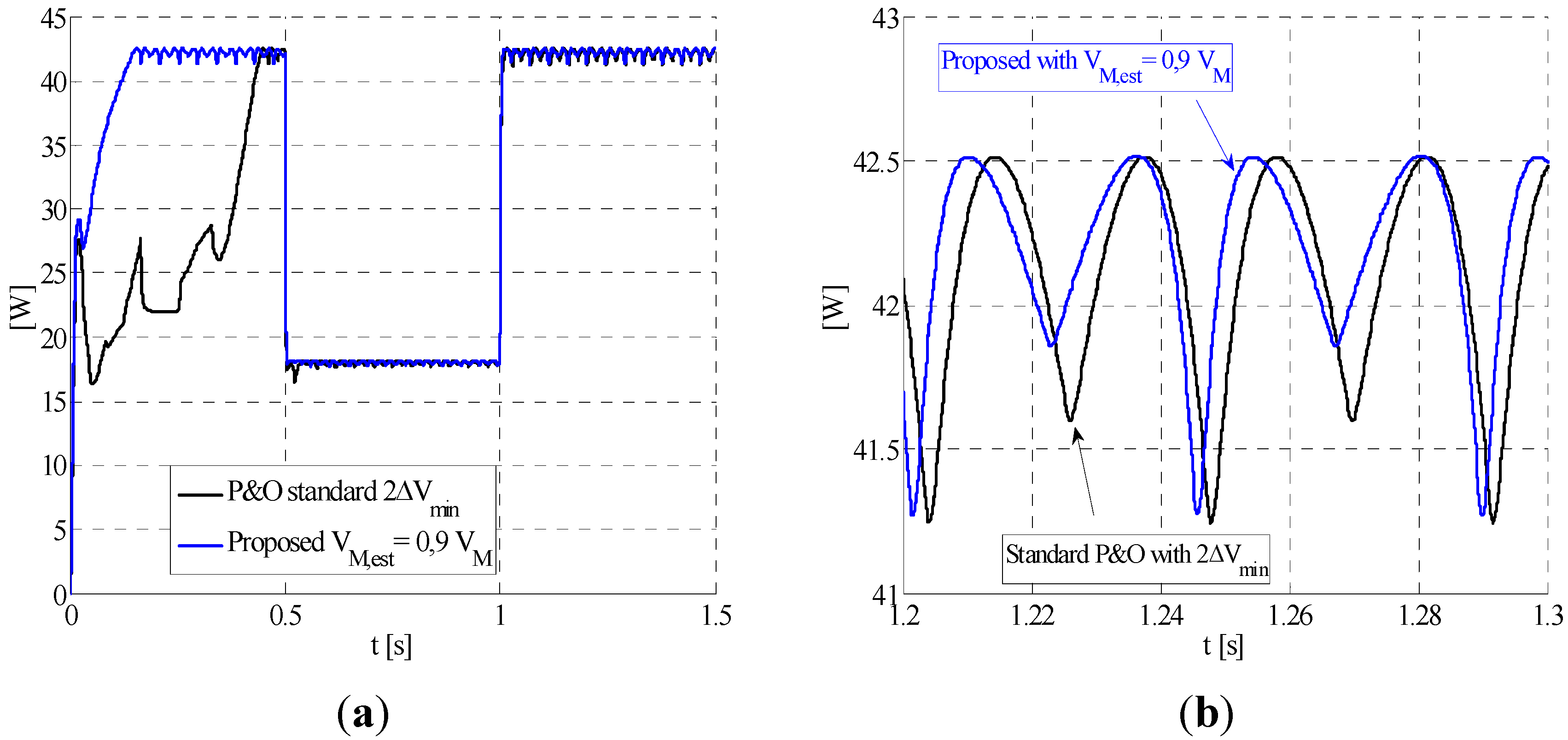
In Figure 17 the best result of traditional P&O algorithm (ΔV = 2 ΔV_min) is compared to the worst case of the proposed algorithm (V_M,est = 0.9 V_M).

From Figure 17 it can be deduced that the proposed algorithm is faster than the traditional P&O method during transient and ensures smaller oscillation in steady-state conditions. As a consequence, the proposed method produces a higher mean power value, even when an estimation MPP error of 10% is introduced.

Figure 17. Comparison of output power between traditional P&O and proposed method with 10% estimation error; complete simulation (a) and steady-state analysis (b).

Figure 17. Comparison of output power between traditional P&O and proposed method with 10% estimation error; complete simulation (a) and steady-state analysis (b).

8. Conclusions

A variation of the classic maximum power point tracking perturb & observe method for photovoltaic power systems has been proposed, implemented and tested. The main limitation of perturb & observe algorithms is the compromise between fast dynamic response and steady-state stability. To improve the dynamic performance and ensure good stability, a criterion for choosing the optimal perturbation step and its coefficients has been discussed. The chosen function enables more flexibility of algorithm to the actual photovoltaic system conditions.

The modified perturb & observe algorithm has been implemented on a dual input inductor push-pull converter and experimentally compared to traditional P&O and IC techniques. For both these algorithms, the perturbation step was adjusted with tuning tests in order to extract the maximum average power from the PV panel and, consequently, penalizing the proposed system in the comparison.

The experimental results have demonstrated clearly that the proposed modified perturb & observe algorithm is better than the standard P&O and IC at steady-state and shows comparable reactivity during transients, even if no adjustment is operated on the perturbation voltage step for different operating conditions. This is due to the intrinsic adaptive characteristic of the algorithm: the perturbation step is higher when the irradiation changes suddenly and is lower when the operating point is close to the maximum power point. From the analysis of the results, it is evident that the proposed perturb & observe algorithm has higher efficiencies than the algorithms already proposed in the technical literature.