Article

Modeling Innovative Power Take-Off Based on Double-Acting Hydraulic Cylinders Array for Wave Energy Conversion

1
Energy Unit, Tecnalia, Mikeletegi Pasealekua 2-Miramon Donostia-San Sebastián, Gipuzkoa E-20009, Spain
2
Automatic Control and Systems Engineering Department, School of Engineering, University of the Basque Country, Alameda Urquijo Bilbao, Bizkaia E-48013, Spain
*
Author to whom correspondence should be addressed.
Energies 2015, 8(3), 2230-2267; https://doi.org/10.3390/en8032230
Submission received: 28 January 2015 / Revised: 27 February 2015 / Accepted: 2 March 2015 / Published: 20 March 2015

Abstract

:
One of the key systems of a Wave Energy Converter for extraction of wave energy is the Power Take-Off (PTO) device. This device transforms the mechanical energy of a moving body into electrical energy. This paper describes the model of an innovative PTO based on independently activated double-acting hydraulic cylinders array. The model has been developed using a simulation tool, based on a port-based approach to model hydraulics systems. The components and subsystems used in the model have been parameterized as real components and their values experimentally obtained from an existing prototype. In fact, the model takes into account most of the hydraulic losses of each component. The simulations show the flexibility to apply different restraining torques to the input movement depending on the geometrical configuration and the hydraulic cylinders on duty, easily modified by a control law. The combination of these two actions allows suitable flexibility to adapt the device to different sea states whilst optimizing the energy extraction. The model has been validated using a real test bench showing good correlations between simulation and experimental tests.

1. Introduction

All Wave Energy Converters (WECs) based on wave activated bodies comprise, among other subsystems, a reaction mechanism moved by wave action, a Power Take-Off (PTO) system and a control system to adjust the dynamic behavior of the WEC to the incident wave conditions [1]. It is widely assumed that one of the key devices of a WEC is the PTO device. This is due to the fact that it is responsible for transforming the mechanical energy of the moving body into electrical energy. In addition, the PTO is used to control the WEC in order to optimize the extraction of wave energy [2,3,4,5,6,7,8,9,10].
Depending on the technology used for wave energy extraction, there are different PTOs, which can be classified into air turbine devices, electrical direct-drive and low and high pressure hydraulic systems based on the pressurization of a liquid flow [11]. The high pressure hydraulic PTO systems offer the advantage of storing large quantities of energy through the use of gas accumulators that allow a smoother power output. In addition, in most cases they can be assembled using components adapted from standard commercial applications fulfilling requirements to endure hard environmental conditions, and that are suitable for being controlled. According to [12], hydraulics are a well-established technology used in many kinds of on and off-shore drive trains, as demonstrated in Pelamis [6], one of the world’s first grid connected wave energy commercial array of WECs. This kind of PTO transforms the incoming power, which is oscillating at low frequency and high torque, into a continuous and relatively high frequency speed, that is usable by alternators.
As a consequence, in the last decade several research papers related to the modeling of hydraulic PTOs concerning wave energy conversion systems have been published. One of the main objectives of these models is to analyze the behavior of the hydraulic PTO before constructing a real device, that is, assessing the PTO efficiency with the aim of reducing hydraulic losses. The PTO model can then be included in the governing equations of a complete WEC, based on a linear time-domain model using the Cummins approach [13]. Furthermore, the ultimate objective for developing these models is to design control strategies in order to obtain the maximum energy extraction from the sea.
Since the first experimental results of a hydraulic system for energy conversion reported by Budals [14] and later extended by Falnes [15], several authors have developed high-pressure hydraulic PTO models using different approaches.
One of the first models for describing the behavior of a hydraulic system to extract energy from the sea was reported by Eidsmoen in their studies of a heaving-buoy wave energy converter [16,17,18]. The model was developed using mathematical equations of the main components included in the hydraulic system, studying the behavior of the WEC using discrete latching control. Other models followed the same basis with extended and improved approaches, like those developed by Falcão [5], Josset et al. [19] and Ricci [8].
Another approach for modeling a hydraulic PTO for Wave Energy Converters is based on the graphical modeling methodology called Bond Graph. This representation is particularly useful when more than one energy domain is involved in the system as in the case of wave energy conversion systems. The model is based on the exchange of energy through bonds. The bonds are associated with a flow variable and an effort variable, and its product being the exchanged power through the components connected by the bond. In the case of hydraulic systems, the flow variable is the volume flow rate, Q, while the effort variable is the pressure, P [20]. This representation for modeling PTO for wave energy conversion has been used by Engja and Hals [21], Bacelli et al. [22] and Kurniawan et al. [23], among others.
The last approach for modeling the hydraulic PTO has been recently stated by Cargo [24] using the Simhydraulic® software (The MathWorks Inc., Natick, MA, USA) based on the Simscape platform product for the Simulink® Physical Modeling (The MathWorks Inc., Natick, MA, USA) family. In a sense, this approach is very similar to the previous one, as every component in the model can interact with the others by exchanging energy through its ports. This approach is very interesting as it offers a library of basic components parameterized according to vendor’s datasheets. A specific model can be developed using these basic components jointly with user-defined components. Moreover, the behavior of the fluid and the effect of the real pipes of the hydraulic system can be taken into account. In this sense, according to Yang et al. [25], the lengths of the pipes not only influence the transient response, but also the power extracted from the sea. However, most of the aforementioned hydraulic PTO models do not consider the pipes and they also assume that the tank or low pressure reservoir is of a sufficient size that its pressure and volume does not change. These assumptions can lead to inaccurate results due to non-modeled effects such as, the oil compressibility inside the pipes, delays to the pressurization of the system, as well as the effects of entrapped air in the oil [26].
This paper describes the development of a complete model of an innovative PTO focused on the latter approach based on a double-acting hydraulic cylinders array for wave energy conversion. This model is an extension of another model in which losses were assumed to be constant and independent of the hydraulic system pressure and flow [27].
The innovation of this hydraulic PTO with respect to other PTO technologies comes from the flexibility to apply a braking force to the mechanical energy provided by the moving part. Generally in current systems, the adjustment of the force applied by the PTO is carried out by modifying the pressure [6,17,28,29] or by modifying the available areas of the hydraulic cylinders to apply a discrete force [30,31]. The PTOs based on the modified area technique use a Discrete Displacement Cylinder (DDC) in order to employ different forces. The PTO described in this work is able to modulate the torque by modifying the force application points of each individual hydraulic cylinder, by modifying the areas on duty as well as controlling the pressure of the high pressure side. The combination of these three actions enables sufficient flexibility to be able to adapt the device to different sea states, through the application of a large number of restraining torques. This factor can help to improve the optimization of the energy extraction.
In this work, a complete model of the PTO is simulated in open-loop control which considers the actual features of valves and hydraulic motor as well as the effects of the pipes, losses and entrapped air in the oil. The objective is to study the behavior of the complete PTO model using known inputs in order to assess its flexibility using different geometrical configurations and different hydraulic cylinders. By providing a full adjusted model of the PTO, the dynamic force can be included in the Cummins equations instead of using damping coefficients to represent the PTO force in the model [32,33,34]. This PTO model, representing the physical prototype, could be used jointly with current WEC technologies, such as Wavebob [35,36,37], Wavestar [38,39] and Waveroller [40] devices as depicted in the submitted patent application [41].
As described in the paper, the model of this PTO is suitably flexible to enable the implementation of different control strategies. On the one hand, by deactivating the valves blocks it is possible to apply declutching control strategies [3], i.e., the hydraulic cylinders can move freely without applying a force during a specific interval of time. On the other hand, by activating all the hydraulic cylinders, the torque arm could be stopped for a specific duration. In this case the force will depend on the pressure of the high pressure side, in relation to the high pressure accumulator. This means that the PTO system can be used to apply latching control strategies [2,16,34,42,43]. This flexibility in the activation and deactivation of the duty hydraulic cylinders also allows the application of variable time-amplitude pulse control strategies [1].
The paper is structured as follows: Section 2 defines the concept and the theoretical behavior of the hydraulic system is completely described. Section 3 introduces the modeling of the hydraulic PTO system, describing the main components. Finally, the model validation is presented in Section 4, where the simulation behavior of the hydraulic PTO model to different inputs is analyzed and the experimental validation is described.

2. Concept of the Novel Hydraulic PTO System

The hydraulic PTO presented in this work (Figure 1), is able to extract energy from the alternating movement of a torque arm, pivoting from point PP. The restraining torque applied by the PTO input depends on four variables: the sum of the active areas of the operating hydraulic cylinders, the pressure of the high and low pressure accumulators, the location of the fixing points of each hydraulic cylinder in relation to the PTO input axis defined in Figure 2, and finally, the status of the control valve.
Figure 1. PTO Hydraulic Scheme.
Energies 08 02230 g001
Figure 2. Parameters defining the position of one of the hydraulic cylinder rod with respect to the pivoting axis (PP).
Energies 08 02230 g002
As Figure 1 illustrates, the hydraulic PTO is comprised of a set of sub-systems: an array of hydraulic cylinders working as displacement pumps and fixed to vertical columns [27,41], a group of valve blocks in order to control the reactive force of the PTO, a High Pressure (HP) accumulator to store the excess energy and provide smoother power output, a control valve that can be actuated in order to regulate the hydraulic flow into the hydraulic motor, a Low Pressure (LP) accumulator to supply oil into the hydraulic cylinders and, finally, several check valves to force the flow of the hydraulic oil in a specific direction. Apart from the check valves included in Figure 1, each valves block contains four check valves as indicated later in this paper (see Section 3.1.2 below). In order to control the temperature of the hydraulic fluid and maintain good operating conditions, several auxiliary components have been included in the hydraulic scheme such as the chiller, two Pt100 temperature transducers and a filter on the low pressure side. In order to clarify the scheme, the different pressure sides have been identified by colors: blue (oil to HP), red (oil to LP from hydraulic cylinders) and green (oil from LP to hydraulic cylinders).
In Figure 2, the geometrical parameters that change the geometry are shown. This figure defines the position of the hydraulic cylinder rod taking into account AC (L), OC and OB (R) distances, the hydraulic cylinder length (AB) and the angular position of the PTO input shaft, Ф. The hydraulic cylinder length, AB, varies with the movement of the PTO input as the rod of the hydraulic cylinder is moving.
The articulated fixing points of the hydraulic cylinders chambers, A points, are fixed in two parallel vertical columns [27]. At a specific value of pressure in the HP accumulator, and in order to quickly apply a higher braking torque additional hydraulic cylinders can be set on duty. If the torque at the PTO input is sufficient to move the rod of the hydraulic cylinders, which is directly related with the pressure of the HP accumulator, then the input flow, Q1, will be propelled into the high pressure side. If the movement of the input shaft of the PTO is able to move the hydraulic cylinder rods, and as long as the control valve is closed, then the high pressure of the system will increase thereby reducing the pressure inside the low pressure accumulator.
The flexibility and precision of this PTO is improved by the inclusion of a mobile electro-hydraulic fixing system at both ends of each hydraulic cylinder. By modifying the parameters OB (R) and AC (L) depicted in Figure 2, the restraining torque changes. On the one hand, moving point A along the AC and, on the other hand, moving point B along OB, the torque arm can be adjusted regarding the requirements of a specific input. These parameters can be adjusted depending on the sea state. Table 1 specifies the geometrical parameters possibilities of each double-acting hydraulic cylinder. The last row of Table 1 represents the available variation of the rod displacement depending on AC, OB and OC parameters in conjunction with the angular position of the PTO input shaft, Ф.
Table 1. Geometrical parameters applied to hydraulic cylinders.
Parameter DescriptionHydraulic Cylinder HC3.1 & HC3.3Hydraulic Cylinder HC3.2 & HC3.4
Maximum admitted Input angle, Ф (°)±26.85±26.85
OC (mm)713700
OB (mm)—Possibilities105/142.5/180/217.5100/140/175/210
AC (mm)—Possibilities30/105/142.5/180/217.530/100/140/175/210
Rod displacement range (mm), fn (OB, AC, OC, Ф cylinder dimensions)93.5–196.589–189.7
These two parameters, OB and AC, in conjunction with the active area, Ai, of each active hydraulic cylinder allow the application of discrete restraining torque at the input of the PTO shaft connected to the Energy Capture Device. Hence, the expression for the restraining torque applied by the PTO is the sum of the restraining torque applied by each hydraulic cylinder:
T = i = 1 4 τ i = i = 1 4 P 1 A i r i = P 1 i = 1 4 A i r i
where P1 is the pressure inside the hydraulic cylinder chamber in service, directly related to the pressure inside the high pressure accumulator; and ri is the torque arm, the distance between the longitudinal axis of each hydraulic cylinder and the pivoting axis, PP, of the input shaft of the PTO.
As seen in Figure 2, the ri parameter is defined by OB (R) and AC (L) parameters and the hydraulic cylinder dimensions, parameter AB, together with the instantaneous angle of the input shaft of the PTO, Ф. This angle can be easily measured in a real time system using a suitable encoder. Knowing this angle and the geometrical parameters identified in Figure 2, through the application of the cosine theorem to calculate φ and θ angles, it is possible to compute the arm of each hydraulic cylinder rod along the time of the hydraulic cylinder rod through the following equation:
r i = O A s e n ( a r   cos ( O A 2 + A B 2 O B 2 2 O A A B ) )
where AB is a function of Ф through the Equation (3):
A B = O A 2 + R 2 2 O A R cos ( π 2 + α Φ )
From the behavior of the rod position with time, it is possible to derive the instantaneous oil flow contribution to the high pressure side. Hence, defining a time interval Δt (t−1 → t), the instantaneous flow can be computed following the Equation (4):
Q t 1   t = A i | A B t 1 A B t | Δ t = A i ( Δ x Δ t ) t 1 t

3. Modeling of the Hydraulic PTO Device

The hydraulic model is implemented using Simhydraulics® and Simulink® software platforms using library blocks and some specific hydraulic blocks developed by the authors in order to represent several parts of the system.
As previously mentioned, Figure 1 describes the main components of the complete model of the hydraulic device. In the following paragraphs the main sub models and blocks are described, and their relevant parameters are specified. The fully assembled PTO hydraulic model is described in Section 3.2. The parameters of each component have been jointly selected from the datasheet of real components along with experimental results [44]. The features related to each component are detailed in the SimHydraulics reference [45]. The reason for choosing the geometrical parameters included hereinafter in the model comes from the need to absorb both an oscillating movement of ±30° at 5 rad/s as a maximum angular speed as well as absorbing up to 16,000 Nm from a specific WEC (for more information see [27]).

3.1. Subsystems and Components

The hydraulic model consists of four double-acting hydraulic cylinders, a set of control blocks for every hydraulic cylinder, a set of hydraulic pipelines to connect every hydraulic cylinder port with the control valves blocks, a set of nineteen check valves, two gas accumulators, a control valve, a fixed-displacement hydraulic motor and a pressure relief valve.
The oil characteristics are included in the model through a specific block which parameterizes its density, kinematic viscosity, Bulk modulus and system temperature. The relative amount of trapped air is adjusted by comparing simulation behavior with experimental tests in the same conditions.
As the goal of this work is to demonstrate the PTO flexibility for applying different restraining torques, the model has been simplified, neglecting auxiliary components of the complete hydraulic PTO system, such as the chiller and filter. The description of each main component is detailed below.

3.1.1. Double-Acting Hydraulic Cylinders Array

The double-acting cylinders array transforms the kinematic energy from the alternating angular movement of the PTO input to hydraulic energy. The motion in both directions is used to pump the hydraulic fluid into the high pressure circuit. The model of these hydraulic cylinders assumes no internal and external leakage. Figure 3 illustrates the connections of every cylinder with the input movement. In this figure, hydraulic connections between cylinders are shown, including pipes and T-junctions.
As can be seen in Figure 3, the same input movement (InputSignal) is applied to every Hydraulic Cylinder (HC) block, whereas every hydraulic cylinder has an independent control input signal to activate or deactivate it, in order to inject flow in the High or Low Pressure side (HP and LP respectively). Figure 3 shows each hydraulic cylinder block connected to the LP, HP and LPr pressure circuits through T-junctions, pipes and cross junctions.
Figure 3. Hydraulic cylinders array model.
Energies 08 02230 g003
Each HC block is modeled including the friction effect between the chamber and the rod. This friction force is simulated as the sum of Stribeck, Coulomb and viscous effects.
Figure 4 shows the model of one of the Hydraulic Cylinder blocks that includes, among other components, the friction effect, pipes between the hydraulic and the valve block ports as well as the motion of the hydraulic cylinder rod through the Kinematic block. Inside the Kinematic block the trigonometric equations deriving the Equation (2) are used to calculate the position and the velocity of the hydraulic cylinder rod, represented as Δx/Δt or v_cili, in Figure 2.
As mentioned previously, this hydraulic model consists of four hydraulic double-acting hydraulic cylinders whose relevant parameters are included in Table 2. These values are selected in order to absorb a maximum torque of 16,000 Nm, as previously indicated.
The use of four double-acting hydraulic cylinders placed in opposite sides having the same area, as indicated in Table 2, offers up to nineteen different areas represented in Figure 5. The use of two identical hydraulic cylinders on opposite sides allows the application of the same force independent of the direction of movement.
The restraining torque depends on the hydraulic cylinders area on duty, the high pressure available in the HP Accumulator, P2; and the torque arm applied by each hydraulic cylinder, ri. This functionality improves the capability of adjusting the restraining force indicated by Hansen [31], who uses three different high pressure accumulators and a multi-chambered hydraulic cylinder to obtain up to thirteen available areas.
Figure 4. Hydraulic cylinder model including each associated elements.
Energies 08 02230 g004
Table 2. Main parameters of the hydraulic cylinders.
Parameter DescriptionH.C. 3.1. and H.C. 3.3H.C. 3.2. and H.C. 3.4
Piston Area A (cm2)8.0419.63
Annulus Area, B (cm2)6.515.83
Hydraulic cylinder maximum stroke (mm)420361
Dead volume Chamber A (cm3)6.75432.452
Dead volume Chamber B (cm3)3.37716.226
Rod Mass (kg)1.112.51
Figure 5. Available areas depending on the hydraulic cylinders on operation.
Energies 08 02230 g005
The availability of these areas together with the possibility of changing the geometrical position of each hydraulic cylinder, as indicated in Table 1, along with the change on the operation pressure allows the application of a greater quantity of restraining torques.

3.1.2. Valve Blocks

These subsystems allow the activation of each hydraulic cylinder independently. The configuration shown in Figure 6 indicates that the fluid flows into the relevant hydraulic cylinder chamber from the LP side (identified as FromLP) and, depending on the state of the 4-way valve, the fluid is pumped into HP side (ToHP) or LP side (ToLP). This operation is very noteworthy: on the one hand, by deactivating the valves block, it is possible to apply declutching control strategies [3], i.e., moving the hydraulic cylinders freely. On the other hand, by activating all of the hydraulic cylinders, the torque arm could be stopped for a specific period. This means that PTO system could be used to apply latching control strategies like the ones proposed by several authors [2,15,34,42,43]. In order to avoid pressure peaks, noise and additional losses, it is recommended to close valves when the speed of the rods is low, i.e., very close to zero.
Figure 6. Valves block model.
Energies 08 02230 g006
Furthermore, the availability of independently activating and deactivating the hydraulic cylinders, allowing up to nineteen different areas, allows the application of control strategies based on variable amplitude pulse control [1].
Each valve block consists of two 4-way directional valves and several check valves. The status of the each directional valve is governed by a 3-position valve actuator. The main parameters affecting this subsystem are indicated in Table 3. The model of these valve blocks subsystems is shown in Figure 6.
Table 3. Valve block main parameters.
SymbolParameter DescriptionValue
CDFlow Discharge coefficient0.65
AmaxFully open valve passage area (mm2)44.18
AleakClosed valve leakage area (m2)2.745 × 10⁻¹¹
TonSwitching-on time (ms)60
ToffSwitching-off time (ms)40

3.1.3. Check Valves

These components allow flow in one direction and block it in the opposite direction. The valve remains closed while the pressure differential across the valve is lower than the valve cracking pressure. The model of the check valve accounts for the laminar and turbulent flows and is monitored by the Reynolds number, Re. If the Re value is below the critical Reynolds number, Recr, the regime is laminar, hence, the flow follows the Equation (5). Otherwise, the regime is turbulent and relates to Expression (6) for the flow governing equation [45]:
q = 2 ( C D Re   c r ) A ( p ) 1 υ ρ 4 A ( p ) π p
q = C D A ( p ) 2 ρ | p | s i g n ( p )
From Equations (5) and (6), the instantaneous orifice passage area, A(p), depends on the differential pressure across the valve, p, as included in [46]. This instantaneous orifice area changes linearly between cracking pressure and the pressure needed to fully open the valve. In Table 4, a description of the main parameters and its corresponding values for the check valves included in the model (see Figure 1) are indicated. Furthermore, all of the assembled check valves inside the Valve Blocks correspond to CV1 type check valves.
Table 4. Check valve main parameters.
SymbolParameter DescriptionValue CV1Value CV2
CDFlow Discharge coefficient0.5350.535
AmaxFully open valve passage area (mm2)126.677660.52
AleakClosed valve leakage area (m2)2.75 × 10−112.75 × 10⁻¹¹
pcrackCracking Pressure (bar)0.171
pmaxPressure needed to fully open the valve (bar)3.4473.447
It is widely assumed to consider this kind of components working under turbulent regime [47,48], therefore the critical Reynolds number, Recr, has been suitable considered in this sense.

3.1.4. Hydraulic Pipelines

The pipelines are used to hydraulically connect different components of the model. The model of this block takes into account friction losses along the pipe length as well as the fluid compressibility.
One type of pipelines is used to connect the hydraulic cylinders pressure ports to the corresponding valves blocks as shown in Figure 4.
Besides these hydraulic flexible pipelines some other rigid pipelines are considered in the model to connect each Valves Block port with the corresponding gas accumulator using mainly T-junctions. These kinds of pipelines are both included in Figure 3 and Figure 4. The main parameters included in the model for each flexible and circular pipeline are inserted in Table 5. The internal surface roughness height has been selected according to [49].
Table 5. Hydraulic pipeline parameters.
Parameter DescriptionH.C. 3.1. to Valve Block 4.1H.C. 3.2. to Valve Block 4.2H.C. 3.3. to Valve Block 4.3H.C. 3.4. to Valve Block 4.4
Diameter (mm)12.719.0112.719.1
Length (mm)3300310040003500
Internal surface roughness height (mm)1.5 × 10⁻²

3.1.5. Pre-Charged Gas Accumulators

An accumulator consists of a pre-charged gas chamber connected to the hydraulic system. If the pressure of the fluid, p, is higher than the preload gas pressure, ppr, the hydraulic fluid will go into the accumulator compressing the gas and storing hydraulic energy through oil volume, VF. If the pressure inside the accumulator is decreasing, it is due to the fact that it is delivering energy to the system.
The model of the gas accumulator assumes a polytropic process, widely accepted by the research community [5,8,17] as being the specific heat ratio, k, 1.4, when nitrogen is considered as the pre-charged gas. As the surrounding air temperature doesn’t change significantly over time intervals less than several hours, it is reasonable to consider that the gas compression/expansion process inside the accumulator is approximately isentropic. This means that the corresponding changes in entropy may be neglected, although the changes in gas temperature inside the accumulator may be significant during the compression/expansion cycle [5]. In this model, the volume inside each accumulator, VF, is governed by Equations (7) and (8) and depends on the structural compliance of the accumulator, Ks. This parameter is introduced in the model to improve the convergence and computational efficiency. In this case it is established at 1 × 10⁻⁸ m3/bar. Equation (8) is applied when the pressure in the inlet of the gas accumulator is higher than the pre-charged pressure. The main parameters are detailed in Table 6.
q = d V F d t
V F = K s p p r { ( p p r p ) 1 k } + V A { 1 ( p p r p ) 1 k }
Table 6. Parameters of pre-charged gas accumulators.
SymbolParameter DescriptionHP AccumulatorLP Accumulator
VAAccumulator Capacity (l)51.551.5
pprPreload pressure (bar)601.5
V0Initial Volume (l)0.00129

3.1.6. Fixed-Displacement Hydraulic Motor

The fixed displacement hydraulic motor is modeled taking into account constant volumetric, ηv, and hydraulic-mechanic, ηmech, efficiencies, the nominal pressure, pnom, the angular speed, ωMH, and several characteristics of the hydraulic fluid such as the fluid kinematic viscosity, υ, and the fluid density, ρ. Hence, the flow through the hydraulic motor is governed by Equation (9) [50], whereas the generated torque is calculated using Equation (10). The main parameters are described in Table 7, where ∆p represents the pressure drop between the inlet and outlet of the hydraulic motor.
Table 7. Fixed-displacement hydraulic motor main parameters.
SymbolParameter DescriptionValue
DMotor displacement (cm3/rev)4.9
ηvVolumetric efficiency0.98
ηmechHydraulic-Mechanical efficiency0.9
pnomNominal pressure (bar)300
ωnomNominal angular velocity (rpm)4500
In between the fixed hydraulic motor and control valve (see Section 3.1.7) is a rigid pipe whose length and diameter correspond to 2500 mm and 8 mm respectively. Under the model of the hydraulic motor subsystem, the possibility to apply a load depending on the status of an input signal has been included. However, for simulations of Section 4, the load only includes the inertia of the output encoder, the coupling and the hydraulic motor inertia, and which totals 1.62 kg·cm2:
q M H = D ω M H + D ω n o m ( 1 η v ) υ n o m ρ n o m υ ρ p n o m Δ p
T M H = D Δ p η m e c h

3.1.7. Control Valve

Although most of the works in the literature use the variable-displacement hydraulic motor as the output of the PTO, this model considers a fixed-displacement hydraulic motor to allow very low flows keeping high efficiency. This is due to the real PTO test bench which has been designed to be tested and used for 1/4 scaled WEC. Therefore, to control the flow rate through the hydraulic motor or its inlet pressure, the model uses a control valve which can adjust the aperture in order to allow variable flow rate. This produces a variable angular speed in the shaft of the hydraulic motor.
The control valve is used to modify the flow through the fixed-displacement hydraulic motor. This kind of component produces heat losses related to the pressure drop and the flow rate through it. However, this valve should be used when it is necessary to control the flow rate or pressure of the system using a fixed displacement motor.
The valve used in the model (2B13N type) is parameterized according to the chart from the datasheet [51], including the evolution of the flow through the valve in Figure 7, and which depends on the percentage of the command signal whereas the pressure drop between the inlet and outlet is about 5 bar.
As shown in Figure 7, the flow through the valve depends on the percentage of the aperture of the valve controlled by a proportional signal. The valve is characterized by a discharge coefficient, established at 0.154 after an iterative process. Several simulations were performed in order to adjust the results from simulations with experimental results. Further explanation of this process is made in Subsection 4.2. In addition, the closed valve leakage area has been established at 9.6 × 10⁻¹¹ m2. This value is related to the internal leakage of the valve when it is completely closed.
Figure 7. Control valve flow versus command signal. Courtesy of Eaton Corporation.
Energies 08 02230 g007

3.1.8. Pressure Relief

The relief valve is a security system to limit the maximum pressure of the hydraulic system. This valve is closed whilst the pressure at the valve input is lower than the limit pressure. If the limit pressure is reached, the flow through the valve will depend on the pressure drop of the valve and the Reynolds number. The main parameters used in the model for this block are indicated in Table 8. The expressions which model this kind of valves are the same as indicated in Equations (5) and (6).
Table 8. Pressure relief valve main parameters.
SymbolParameter DescriptionValue
CDFlow discharge coefficient0.535
AmaxFully open valve passage area (mm2)96.94
AleakClosed valve leakage area (m2)9.6 × 10⁻¹¹
psetValve pressure setting (bar)200
PregValve regulation range (bar)5

3.2. Assembled Subsystems and Components

Taking into account the previous description of the subsystems and components, the complete model is depicted in Figure 8. The model monitors the main flows and pressures of the hydraulic system using flow and pressure gauges. These elements have been identified as QS and PS in the model, respectively. In addition, the model monitors the angular speed and torque of the PTO input, TorqueArm_Speed, and T_PTO signals respectively. In this sense, in addition to the pressure of each hydraulic cylinder chamber, the pressure of the HP and LP accumulators, the flow generated by each cylinder on duty and the flow supplied to each gas accumulator and through the hydraulic motor are monitored in the time domain. Moreover, the average value of the flow supplied by the hydraulic cylinders on duty is calculated based on a continuous data buffer regarding the instantaneous flow. This average flow could be used, in the future, for appropriately opening the aperture of the control valve thereby supplying a specific flow to the fixed-displacement hydraulic motor.
Figure 8. PTO hydraulic model assembled.
Energies 08 02230 g008
The model of the system in Figure 1 is further depicted in Figure 8. The hydraulic model includes, on the left hand side of the schematic, the double-acting cylinder array system. This block has five inputs: the Input signal, corresponding to the displacement of a rack-pinion movement, and the control signals activating and deactivating each hydraulic cylinder through an ON/OFF command to obtain different available areas. In the middle of the schematic are the gas accumulators and a virtual sensor which calculates the mean value of the flow pumped by the double-acting cylinder array system. Furthermore, the relief valve is located close to the LP Accumulator. Finally, on the right hand side of the schematic, the fixed-displacement hydraulic motor, the control valve and the check valve, called CV2 in Figure 1, are represented. The outputs of this open loop model are identified in Figure 8 as MH_Speed and MH_Torque, the speed and torque of the hydraulic motor, respectively.
The last point to completely define the hydraulic model is related to the hydraulic fluid characteristics and the Solver. In order to evaluate the model, it is necessary to include two more blocks, the Solver and the hydraulic fluid that goes through every component. Table 9 indicates the main features of the hydraulic fluid established in the model.
Table 9. Hydraulic fluid parameters.
Parameter DescriptionValue (25 °C)
Density (Kg/m3)876.087
Fluid kinematic density (cSt)97.22
Relative amount of trapped air0.06
Bulk modulus (Pa)1.6 × 10⁹

3.3. Model Input and Output Signals

Taking into account that the final goal is to adjust the model with the assembled PTO (see Section 4), an input motion signal has been chosen instead of an input force signal. The completely adjusted model will be used in future works focusing on the dynamic behavior of the complete WEC-PTO system.
In order to analyze the behavior of the PTO model, its input motion is modeled using the kinematic scheme depicted in Figure 2. Moreover, the generation of the alternative angular movement is carried out through a linear movement generated by a rack-pinion geared system using a 96 mm primitive diameter, Rp, as explained in [27]. The model allows connecting/de-connecting hydraulic cylinders off-line or during simulations. It is also possible to define pre-programmed sequences of activation.
According to Figure 2, to apply the input movement signal to each piston rod, AB(t), a linear sinusoidal movement applied in the rack-pinion geared system is transformed into the angular movement, Ф(t), through the primitive diameter. Considering the geometrical parameters of the hydraulic cylinders, characterized by their lengths and the fixation points of their clamping system with respect to the pivoting axis, PP, (dimensions AC, OB and OC), the Ф(t) movement is applied to point B of each hydraulic cylinder rod modified with time along the segment AB. Hence, the applied movement in the hydraulic piston rods follows the Equation (3), where Φ is a function of time (t) following the Expression (11), with A being the amplitude of the sinusoidal movement applied in the rack-pinion system, and f the frequency of the input signal:
Φ ( t ) = A R p s e n ( 2 π f t )
Therefore, following Equations (2) and (3) and substituting Ф using Equation (11), the Torque Arm value of each hydraulic cylinder rod follows the trajectory depicted in Figure 9. These trajectories are followed when the cylinders are placed as in Configuration 1 (see Table 10) and the sinusoidal movement in the rack-pinion system has an amplitude of 40 mm at 0.1 Hz.
Figure 9. Torque arm position versus time of the array cylinders using Config 1.
Energies 08 02230 g009
Table 10. Geometric parameters of the hydraulic cylinder fixation for model validation.
Geometric Configuration UsedOB (mm)AC (mm)OC (mm)
Config 1HC3.1/HC3.3217.530713
HC3.2/HC3.421030700
Config 2HC3.1/HC3.3217.5217.5713
HC3.2/HC3.4210210700
Config 3HC3.1/HC3.310530713
HC3.2/HC3.410030700
Config 4HC3.1/HC3.3142.5142.5713
HC3.2/HC3.4140140700
The developed model analyzes the outputs of the hydraulic PTO model, in response to the input movement. This refers to the pressure inside the high pressure accumulator as a value related to the stored energy and the speed as well as the torque produced by the fixed-displacement hydraulic motor when there is a flow through it due to the opening of the control valve by a given percentage.

3.4. Other Considerations

The model assumes that the temperature in the hydraulic fluid does not change during the simulation. However, it takes into account several parameters that consider most of the hydraulic losses caused by the hydraulic pipes and components including the real characteristics of the hydraulic fluid.
The solver used in the simulations is an implicit continuous variable-step solver, ode15s. It has been selected due to its suitability to solve numerical differential formulas (NDFs). To achieve the best balance between accuracy and simulation time some simulations were carried out using different solver configurations. The best results in terms of accuracy with respect to experimental results were obtained using a relative tolerance of 1 × 10⁻⁴ using an adaptive algorithm, and applying a second order in the numerical differential formulas applied by the solver.

4. Model Validation

The aim of the model validation is to adjust the model parameters through experimental data in order to obtain a complete adjusted open loop model for use in the control of any WEC that generates an alternative angular movement. Therefore, in this section some simulation results are presented in order to check the behavior of the pressure depending on geometrical parameters as well as the hydraulic cylinders on duty through consideration of a specific input movement. The validation demonstrates some of the possibilities to adjust the restraining torque depending on the hydraulic cylinder geometrical configuration and the number of hydraulic cylinders on duty. In addition some simulation tests on the PTO output are displayed, at different percentages of the aperture of the control valve, in order to check the speed of the hydraulic motor.
Firstly the capabilities of this hydraulic PTO through simulation tests are presented, and, secondly, the comparison between the simulation and experimental results after the adjustment of the main features of the components of the model are explained.

4.1. Simulation Validation

With the aim of checking the behavior of the PTO model, different simulations have been carried out using the geometrical configurations indicated in Table 10 whilst applying the same input movement signal.
For the sake of the validation, and later on, the adjustment of the model, a sinusoidal input signal with an amplitude of 40 mm at 0.1 Hz has been selected to move the rack-pinion geared system. In Table 10 the values of the parameters OB (R), AC (L) and OC of each hydraulic cylinder for the selected configurations are defined. The values of each geometrical configuration used in this article correspond to maximum (Config 2), minimum (Config 3) and medium (Config 4) available distances for the OB and AC parameters. Config 1 corresponds to the geometrical configuration used in the experimental tests (see Section 4.2). For simplicity, these values are selected at the beginning of the simulation.
The configurations are related to the maximum displacement, AB, allowed for the hydraulic cylinder rod and previously indicated in Table 1. In this sense, Config 1 allows greater displacement than Config 2, which in turns is greater than Config 4. The lowest allowed displacement is applied by Config 3. The movement directions of points A and B are displayed in 
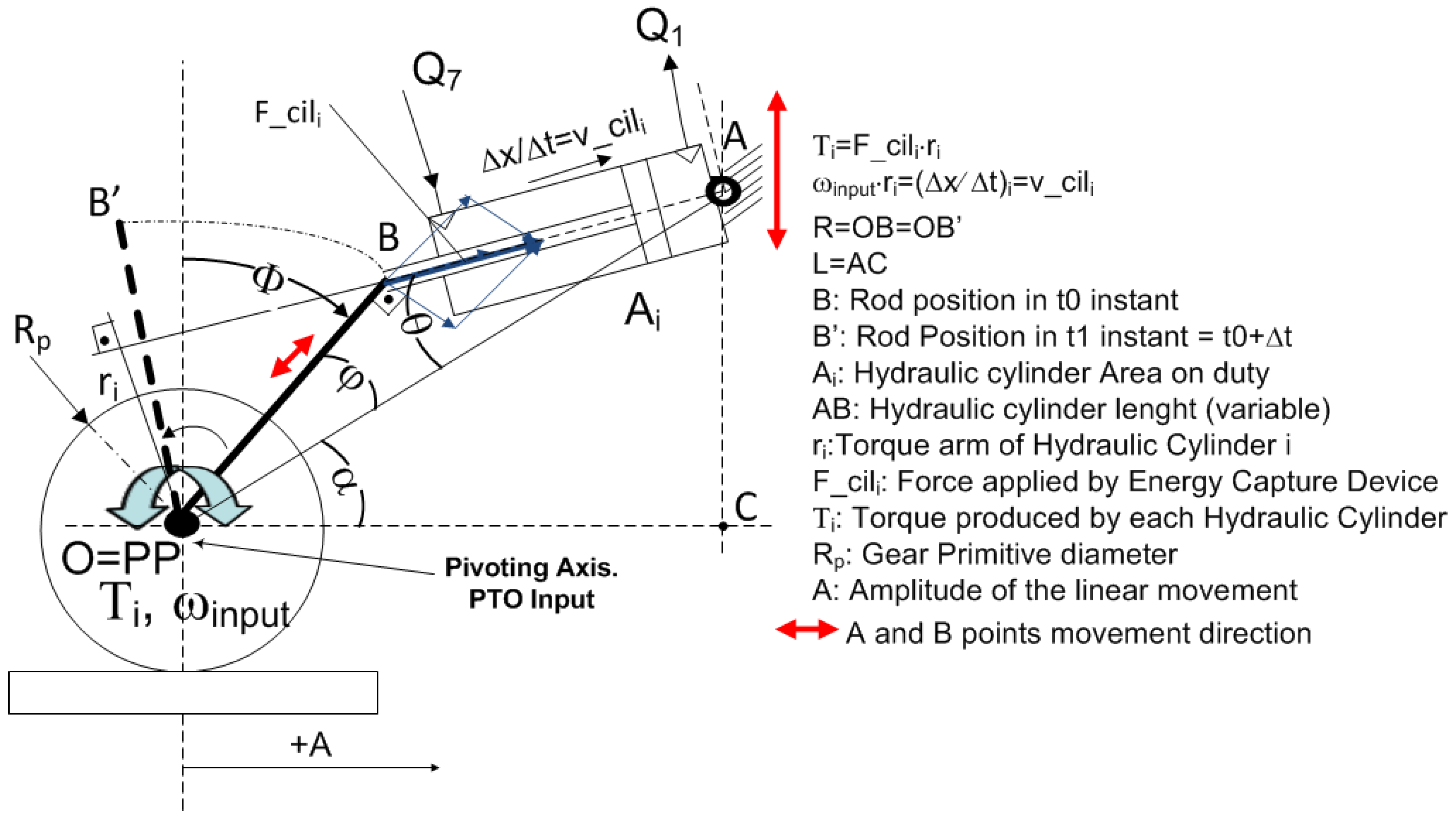
Figure 2 and can be globally seen in [27].
In the model, the different geometrical configurations available for each hydraulic cylinder are discrete (see Table 1). These geometrical configurations could be modified automatically during the operation. Depending on the reaction forces to be supported the choice of each geometrical configuration in the PTO could be driven by electromechanical or hydraulic devices in real application, as indicated in the submitted patent [41]. In the simulations, for validation and experimental tests, these configurations are modified manually at the beginning of each simulation.
The following subsections describe the simulation test performed to check the behavior of the PTO in three different scenarios related to the control valve state: Control valve completely open, control valve completely closed and, finally, control valve opened at some specific aperture percentage.

4.1.1. Simulation Test I: PTO Behavior Using Fully Open Control Valve

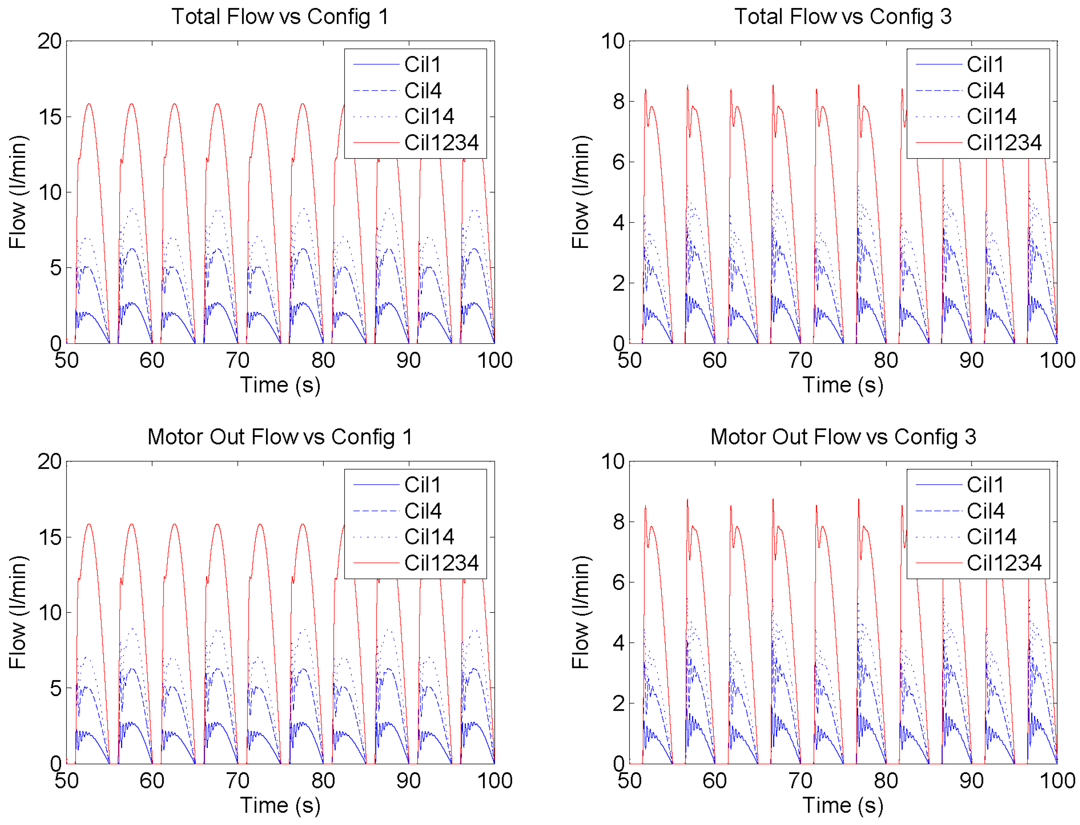
These simulation tests consist of applying a sinusoidal input signal maintaining the control valve completely open. This means that the aperture percentage of the control valve remains at one hundred. In this case, the flow injected by the active hydraulic cylinders will be transmitted completely at the PTO output, except for any leaks within the circuits. The flow through the fixed-displacement hydraulic motor will have a very similar shape when compared to the injected flow rate.
Figure 10 shows the behavior of the input and output flows of the PTO for a specific time and when two geometrical configurations are used (Config 1 and Config 3). The behavior of the flow depends on the activated hydraulic cylinders. The upper left area of Figure 10, shows the instantaneous oil flow injected in the HP side of the circuit with four different activated hydraulic cylinders and using a geometrical configuration that allows high axial displacement of each cylinder rod (Config 1). In the bottom left area of the figure, the flow through the hydraulic motor is shown. The upper right side of Figure 10 shows the instantaneous oil injected in the HP side of the circuit by activating the same cylinders but using a geometrical configuration which allows low axial displacement of each cylinder rod (Config 3). In the bottom right side of the figure, the flow through the hydraulic motor is shown. As Config 1 enables higher rod displacements than Config 3, the injected flow to the high pressure side is higher. As can be seen in the Figure 10, the flow is asymmetrical during one cycle in Cil1, Cil4 or Cil14 cases. This is due to the differences between the piston and annulus areas of each hydraulic cylinder. Hydraulic cylinders with the same characteristics are placed on opposite sides. Therefore only when both of the same characteristics are active will the maximum flow be the same, and independent of the movement direction. This occurs when hydraulics cylinder HC3.1 and HC3.3 or HC3.2 and HC.34 are active. One particular case is shown in Figure 10, where all hydraulic cylinders are activated. The upper and lower graphs are very similar, because the only difference between them is the leakage in the circuit. The sharp peaks of each configuration are related to the inclusion of the pipes in the hydraulic model. According to [25], the inclusion of pipes decreases the stiffness of the hydraulic pump system, in our case the hydraulic cylinders on duty, which can cause a phase delay from the pumped fluid. The longer the length of the pipes, the higher the dead volume of the hydraulic circuit and the lower the stiffness. As indicated in Section 4.2, the amount of trapped air is estimated at around 6%, which further reduces the stiffness of the system. This effect is more pronounced if the hydraulic cylinders on duty are the smallest ones because the hydraulic cylinder chamber volume is lower than the dead volume.
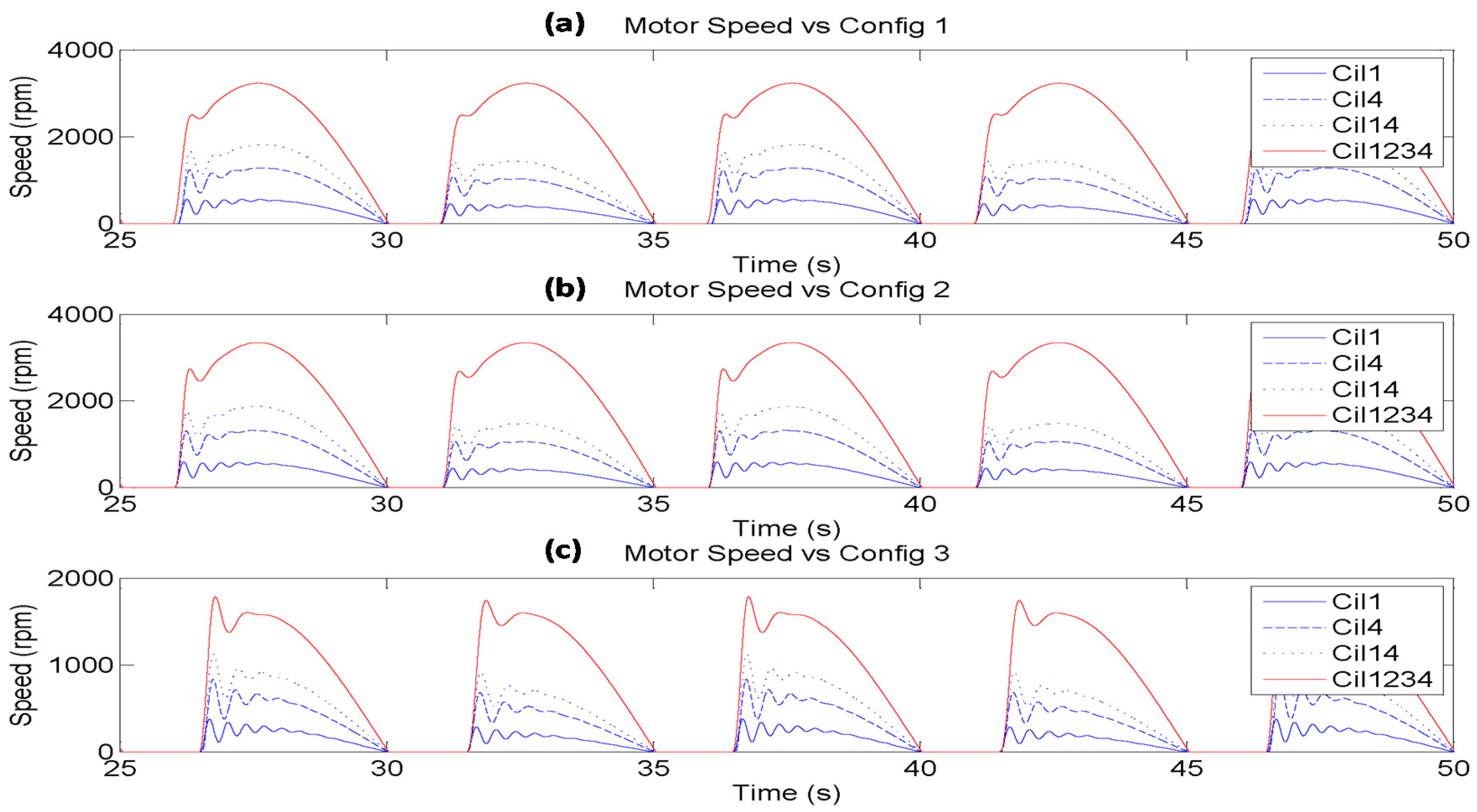
The flow through the fixed-displacement hydraulic motor allows the rotation of the hydraulic motor axis proportionally to the displacement. Figure 11 illustrates the behavior of the hydraulic motor speed in the same configurations using identical active hydraulic cylinders. In this case, three different geometrical configurations are shown; the two previous configurations (a and c graphs) and also the configuration with the highest rod displacement of the hydraulic cylinders (Config 2).
Figure 10. Instantaneous flow at the PTO input and output versus activated cylinders using configuration 1 and 3.
Energies 08 02230 g010
Figure 11. Instantaneous hydraulic motor speed versus activated cylinders using different configurations: Config 1 (a), Config 2 (b) and Config 3 (c).
Energies 08 02230 g011
In this arrangement the movement of the hydraulic cylinder rods using Config 1 and 2 provoke a very similar angular speed in the hydraulic motor. Hence, the angular speed at the hydraulic motor shaft will be very similar.
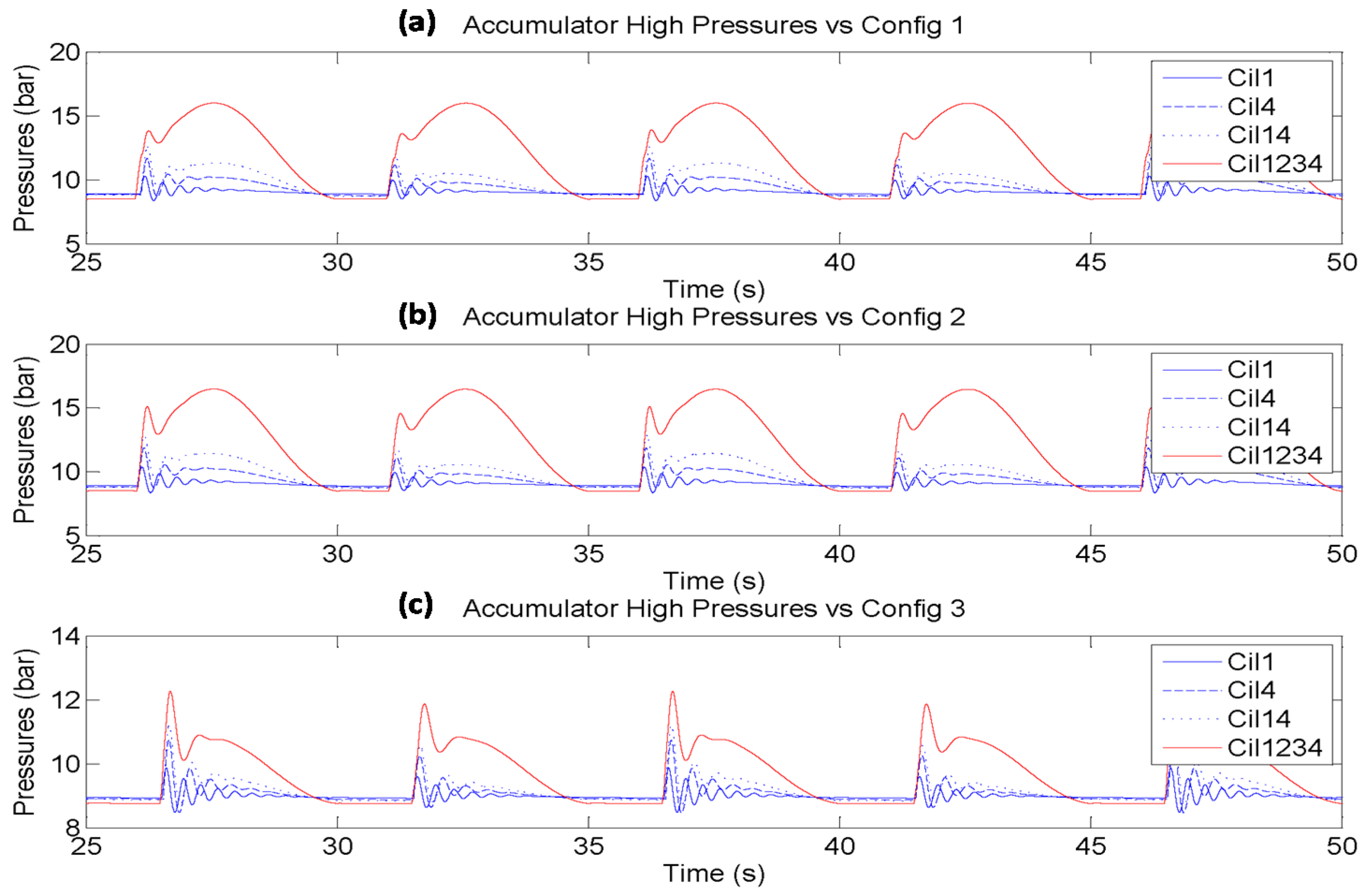
Figure 12 depicts the behavior of the instantaneous HP Accumulator pressure using identical active hydraulic cylinders in the same geometrical configurations from Figure 11. As mentioned before, the sharp peaks of each configuration are related to the pipes included between the hydraulic cylinders and the accumulators. These components reduce the stiffness of the hydraulic system.
Figure 12. Instantaneous HP Accumulator pressure versus activated cylinders using different configurations: Config 1 (a), Config 2 (b) and Config 3 (c).
Energies 08 02230 g012

4.1.2. Simulation Test II: PTO Behavior Using Control Valve Completely Closed

These simulation tests consist of applying a sinusoidal input signal whilst maintaining the control valve completely closed. This means that the aperture percentage of the control valve remains at zero. In this case, the flow injected in the HP side of the hydraulic circuit by the active hydraulic cylinders is stored inside the HP accumulator itself. As the oil volume inside the accumulator is higher than previously, the internal pressure in the accumulator, P2, will increase. These simulation tests demonstrate the flexibility to modify the HP accumulator pressure evolution, on the one hand, depending on the geometrical configuration whilst a specific combination of hydraulic cylinders are active and, on the other hand, depending on the active hydraulic cylinder whilst a specific geometrical configuration is fixed.
As in the previous tests, several geometrical configurations have been selected to show the behavior of the HP accumulator. In this simulation, the relief valve has been fixed at 130 bar. Therefore, if the oil volume inside the HP accumulator reaches to a specific value that exceeds 130 bar, any subsequent input movement will overcome the relief valve pressure. In this case, the injected flow will go through the relief valve, maintaining the same high pressure unless input conditions change.
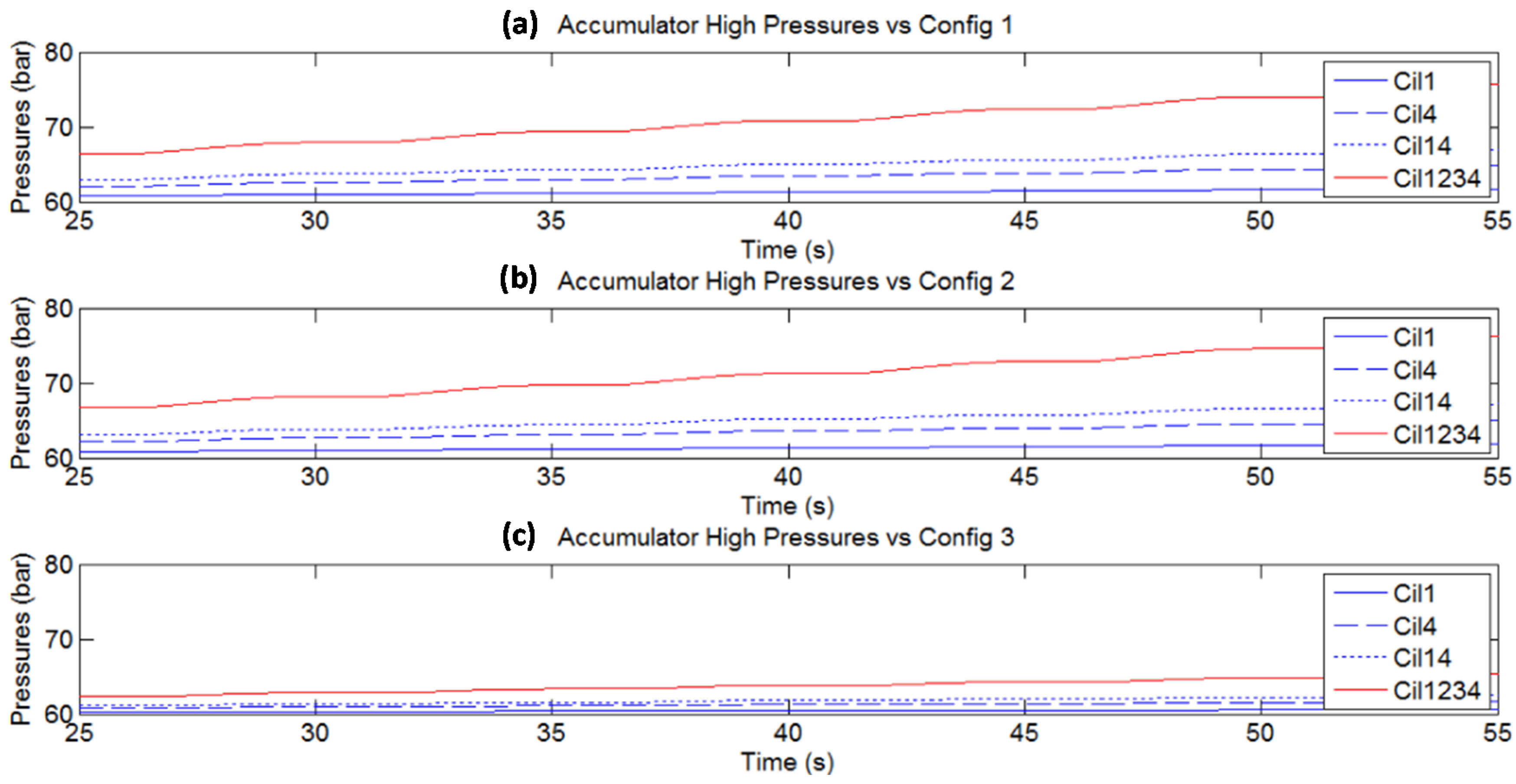
Each graph from 
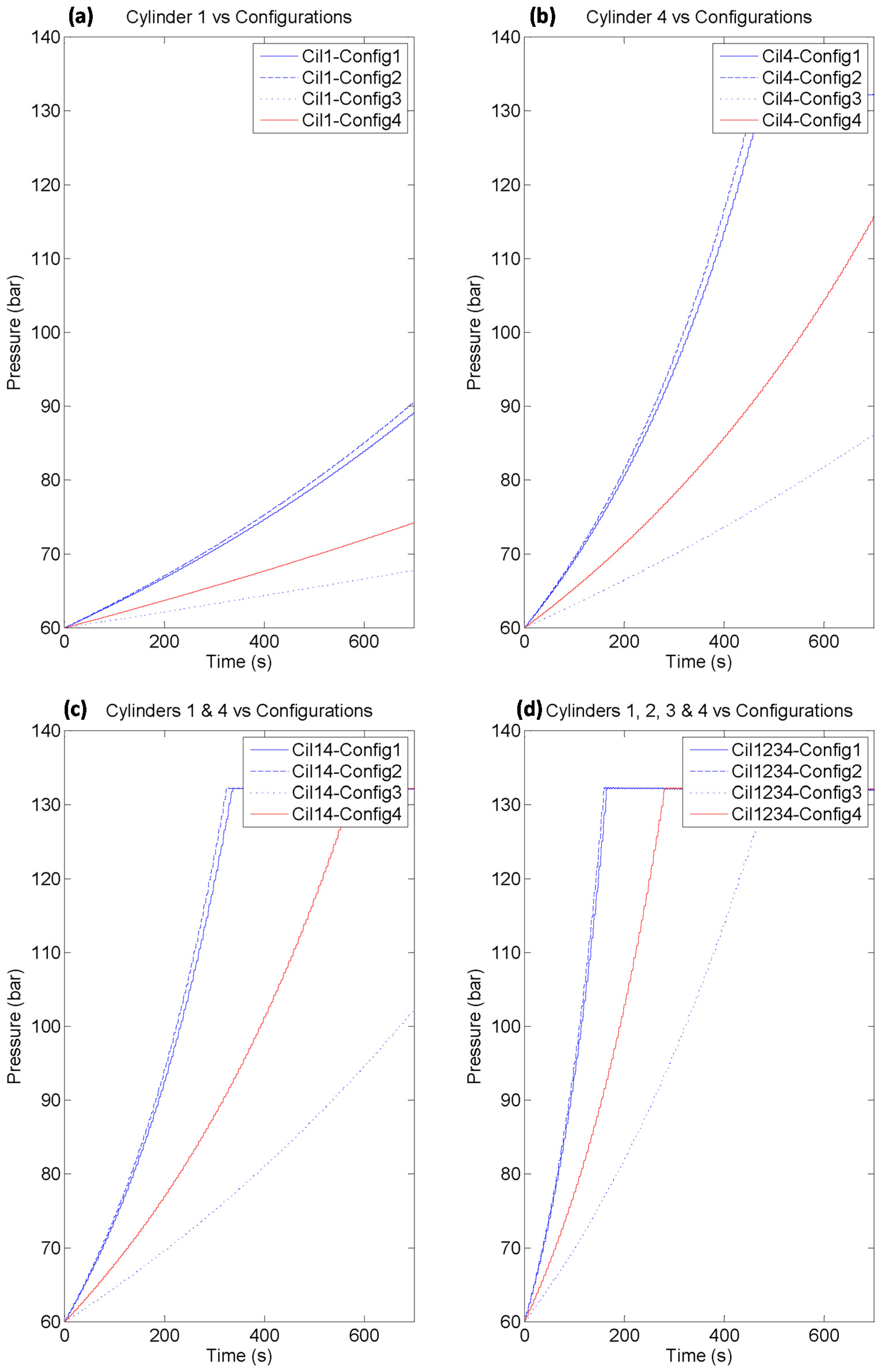
Figure 13 illustrates the evolution of the HP accumulator pressure maintaining the same hydraulic cylinder configuration active, whilst the geometrical configuration changes. When a specific hydraulic cylinder is active, the evolution of the HP accumulator pressure rate depends on the selected geometrical configuration. This fact is related to the maximum displacement allowed by each configuration. Config 1 will reach the required operation pressure faster than the other configurations.
Figure 13. HP accumulator pressure evolution related to geometrical configuration, using a specific combination of active hydraulic cylinders. (a) Cylinder 1; (b) Cylinder 4; (c) Cylinders 1 and 4; (d) Cylinders 1, 2, 3 and 4.
Energies 08 02230 g013
Each graph in 
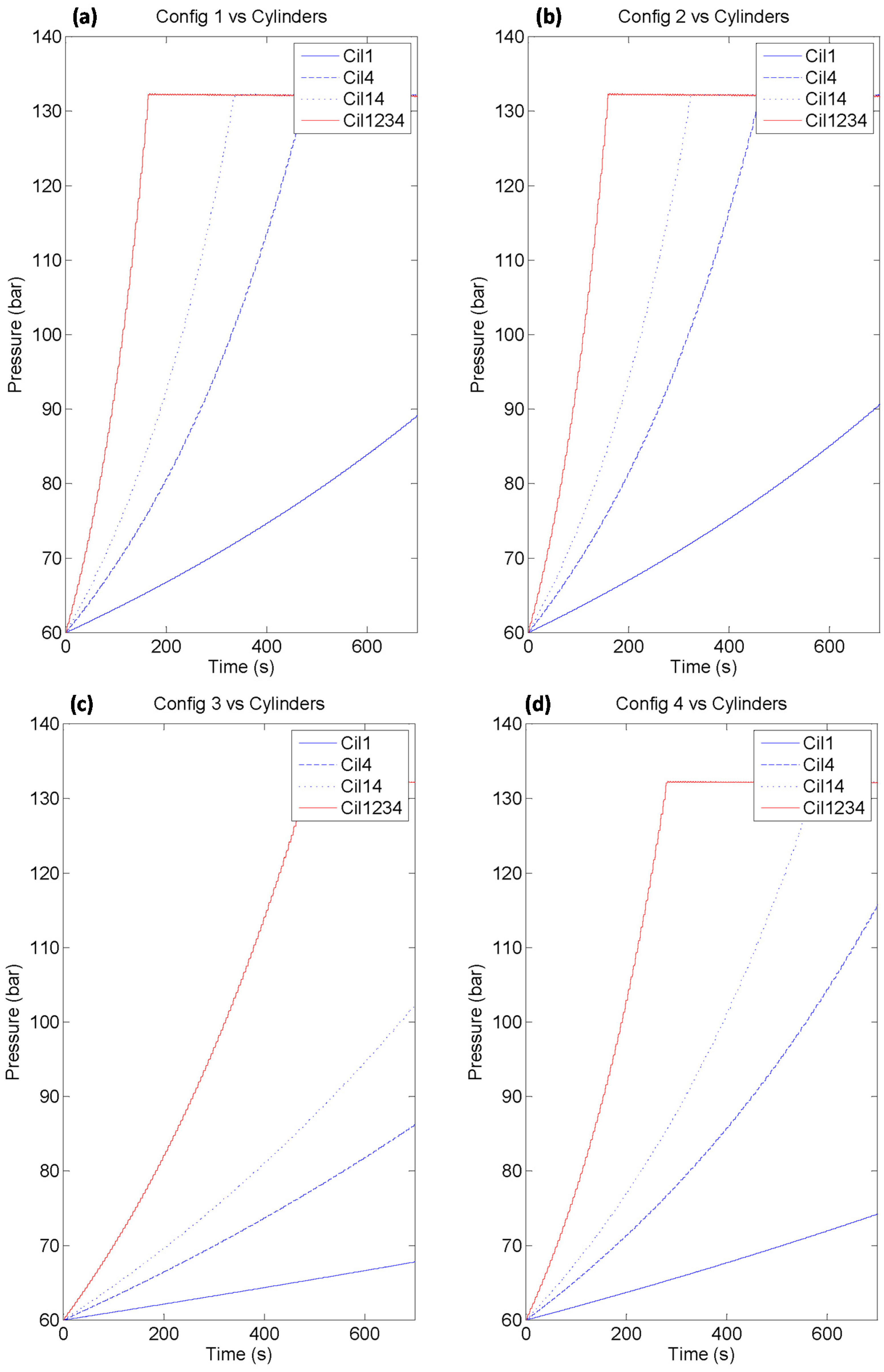
Figure 14 shows the behavior of each geometrical configuration when different hydraulic cylinders are activated. In this case, it is obvious that higher the number of activated hydraulic cylinders, the higher the rate of pressure evolution.
Figure 14. High Pressure accumulator pressure evolution related to the active hydraulic cylinders, with a fixed specific geometrical configuration. (a) Config 1; (b) Config 2; (c) Config 3; (d) Config 4.
Energies 08 02230 g014
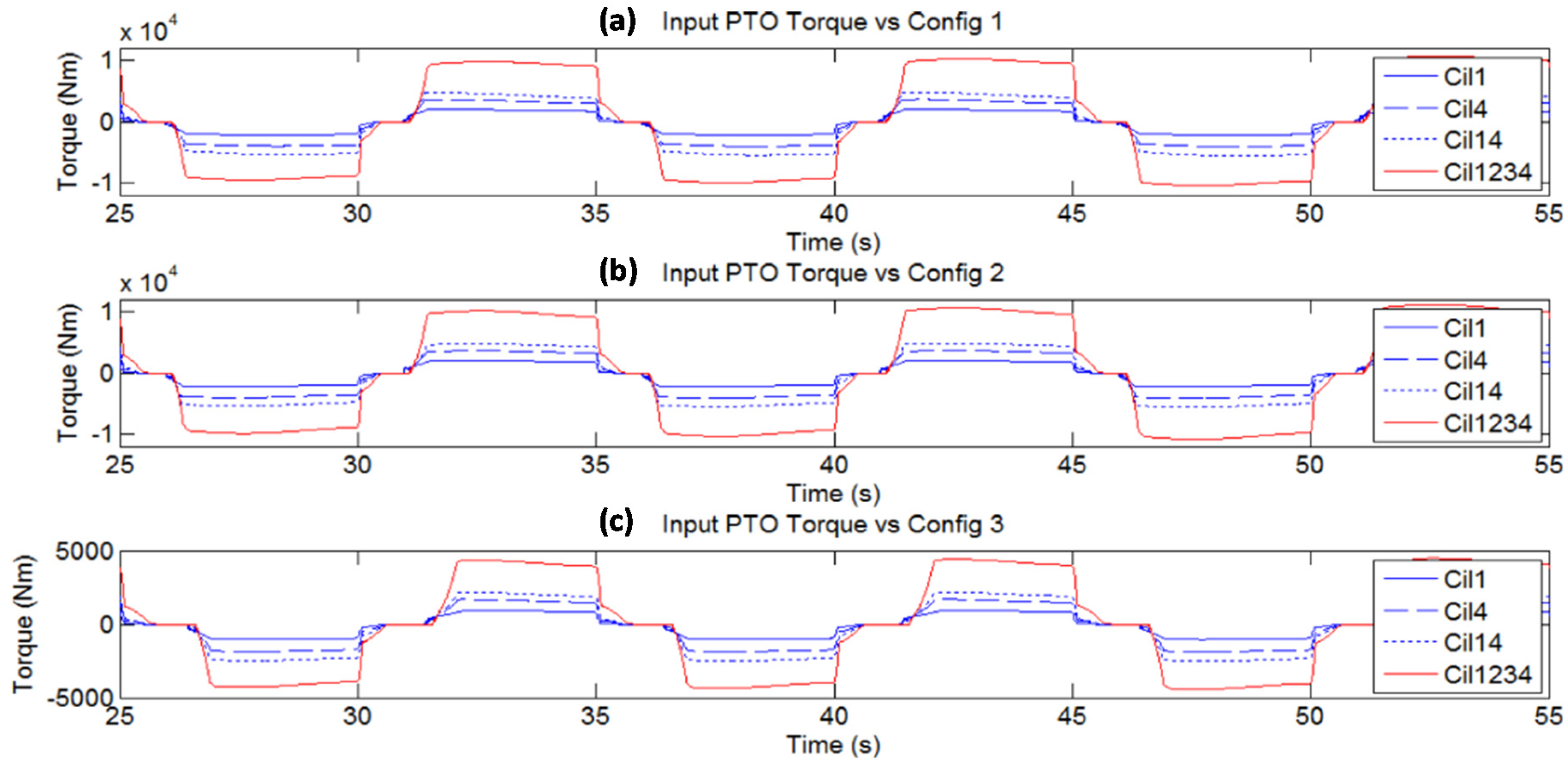
The pressure established at the HP accumulator, in conjunction with the area of the active hydraulic cylinders, allows the application of the restraining torque which will be used to brake the hypothetical wave energy capture device. 
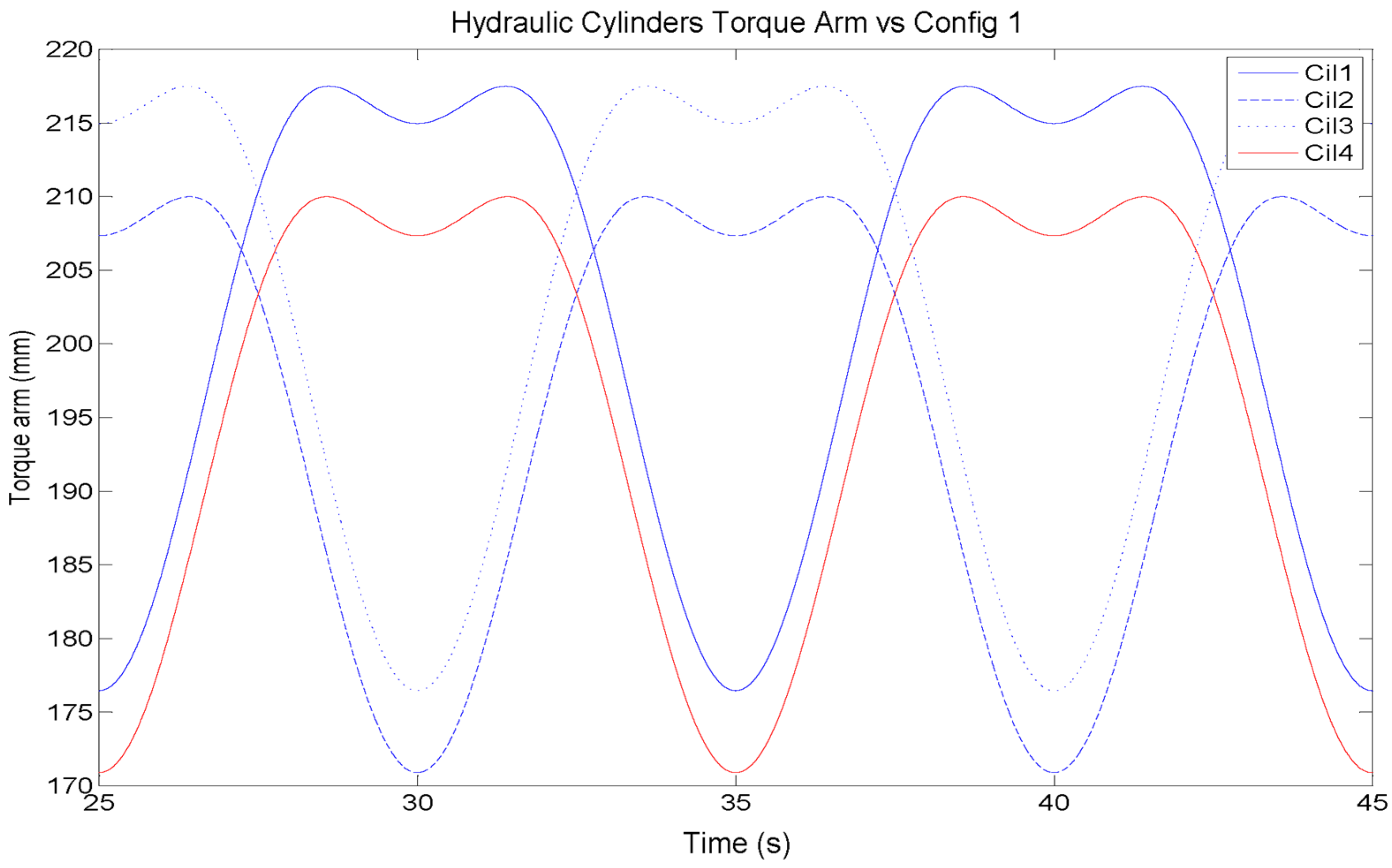
Figure 15 shows the evolution of the alternative restraining torque applied by the PTO input depending on the geometrical configuration and the active hydraulic cylinders. The shape of the plot of the torque against time is similar to the one of a Coulomb-type load. However in this case the restraining torque is modified by changing the areas and the geometrical parameters of the location of the hydraulic cylinders, AB and OB, with respect to the pivoting point, PP.
Figure 15. Restraining Torque Evolution at the PTO input. Comparison between different Geometrical configurations using same activated hydraulic cylinders. (a) Config 1; (b) Config 2; (c) Config 3.
Energies 08 02230 g015
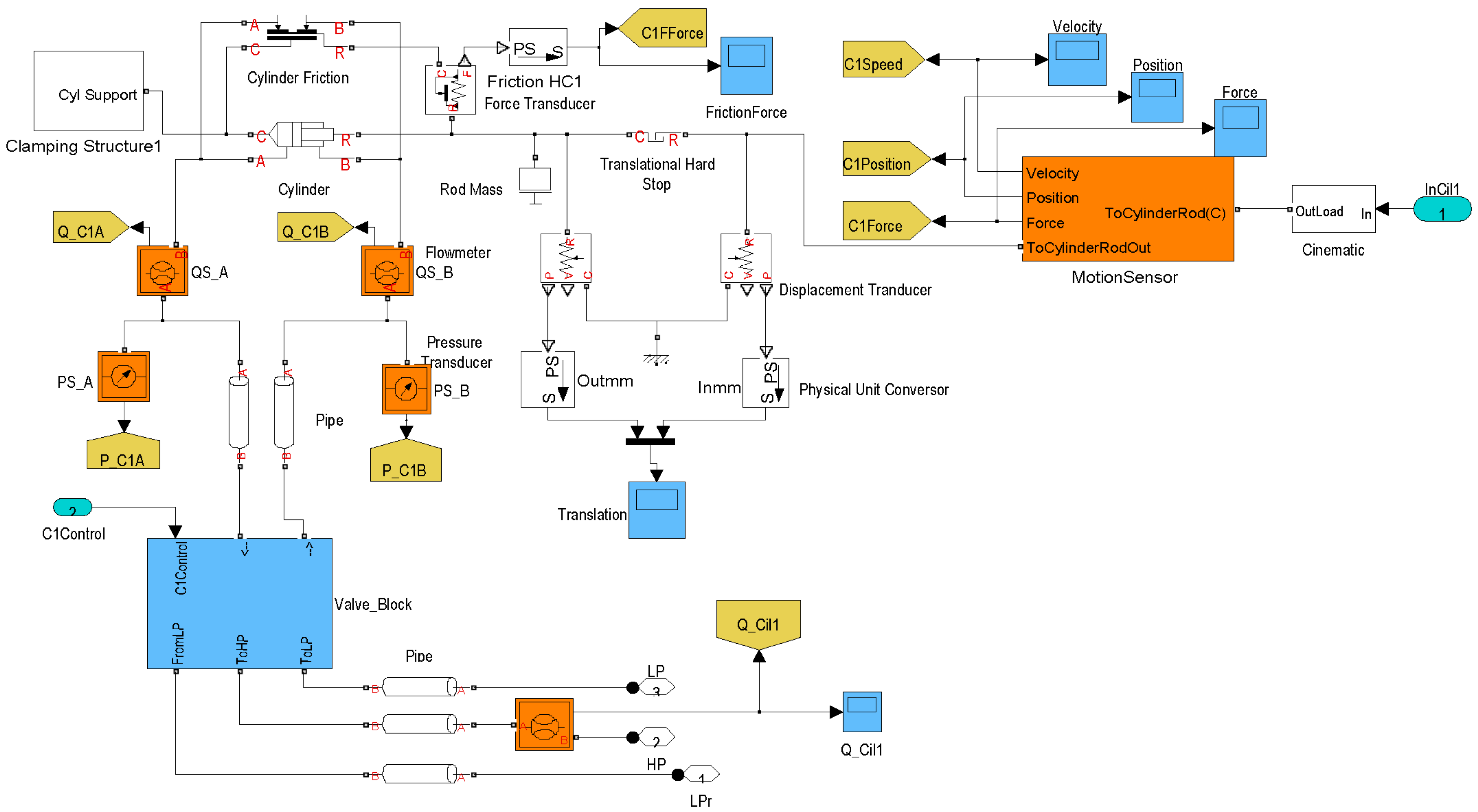
As can be seen, the higher the number of active hydraulic cylinders, the higher the restraining torque. Moreover, using the Config 1 geometrical configuration, a higher restraining torque than other configurations is obtained. In addition, it can be seen that by using lower displacements of the hydraulic cylinder rod (associated with configuration layout Config 3) the time in which the restraining torque is applied is reduced. This is due to the fact that the rod fixation of each hydraulic cylinder includes a translational hard stop, which restricts the motion of the rod between two limits reproducing a certain mechanical backlash. Furthermore, in Config 3, the restraining torque decreases when compared to other configurations. This is due to the fact that the torque arm is smaller than in Config 1, following the Equation (1). The inclusion of the translational hard stop block in the model (see Figure 4) might provoke the appearance of 45° lines when the velocity approaches zero.
Figure 16 shows the HP Accumulator pressure evolutions when the restraining torques depicted in Figure 15 are generated. The pressure evolution of the HP Accumulator is very low, so the restraining torque appears to be the same throughout the simulation. Although it has not been included in the graphs, the LP accumulator pressure decreases from approximately 8 bar in accordance with the oil supplied to the HP side.
Figure 16. HP accumulator pressure Evolution. Comparison between different Geometrical configurations using the same activated hydraulic cylinders. (a) Config 1; (b) Config 2; (c) Config 3.
Energies 08 02230 g016

4.1.3. Simulation Test III: PTO Behavior Using Variable Aperture of Control Valve

These simulation tests consist of applying the same sinusoidal input signal but keeping the control valve open at a certain aperture percentage after a certain programmed time. To carry out these simulation tests two hydraulic cylinders have been considered as active. In this case, one of the small cylinders (HC3.1) and one of the big cylinders (HC3.4) have been selected to pump the oil volume to the high pressure side. The simulations have been performed using the geometrical configuration, Config 1.
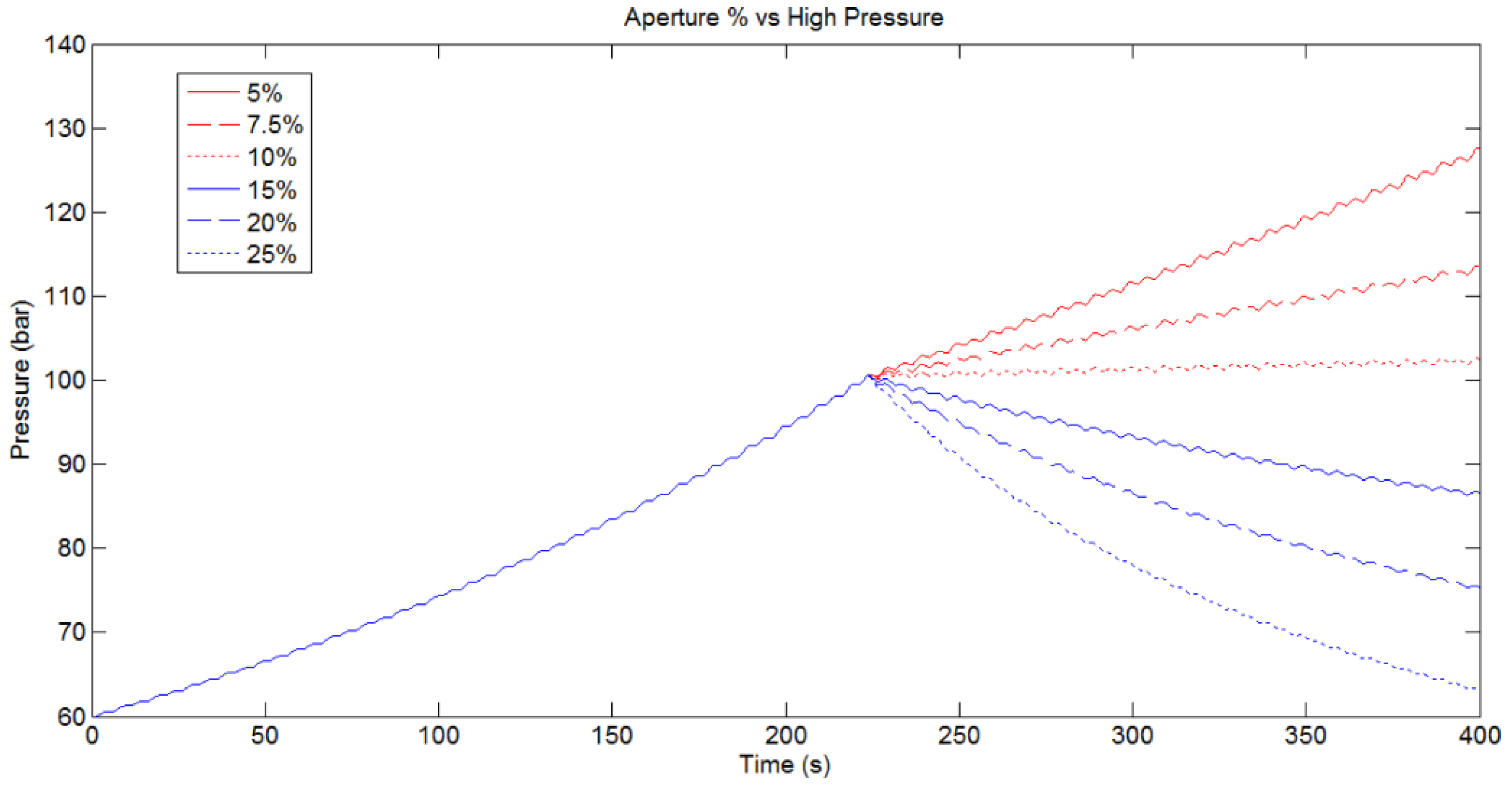
Figure 17 shows the evolution of the HP accumulator pressure, overlapping up to six different control valve percentages. All the simulations open the control valve when the pressure of the HP accumulator reaches 100 bar.
Figure 17. HP accumulator pressure Evolution. Comparison between different control valve apertures using the same activated hydraulic cylinders (HC3.1 and HC3.4). Config 1.
Energies 08 02230 g017
The figure shows that control valve aperture percentages below 10% receive an increment in the HP accumulator pressure whilst maintaining the same PTO input movement. Using control aperture percentages above 15% produces a decrement in the pressure of the HP accumulator. In the first case, the oil volume injected by the active hydraulic cylinders is higher than that demanded by the aperture of the control valve. Therefore the extra flow pumped by the hydraulic cylinders displacement is stored in the HP accumulator. In the other case, as the PTO input movement is not able to supply all the flow demanded by the control valve, the HP accumulator supplies a certain quantity of the stored oil volume to compensate for the lack of flow demanded by the control valve.
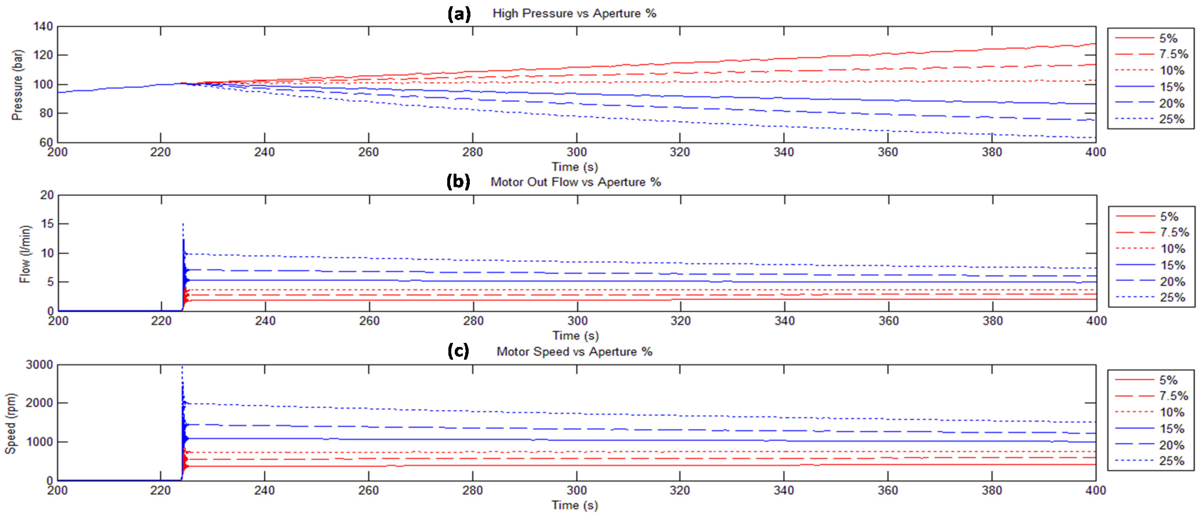
Figure 18 includes the flow through the hydraulic cylinder (L/min) and the hydraulic motor speed (rpm) between 200 and 400 s. The evolution of the pressure of the HP Accumulator, P2, is also shown. In this figure the speed of the hydraulic motor is proportional to the flow through the hydraulic motor according to the Equation (9). As the aperture percentage of the control valve is constant, the speed of the hydraulic motor is practically constant in each case due to the fact that the second term of the Equation (9), representing its leakage, is very small. In these simulation tests, it is important to remark that the LP accumulator pressure is increasing as the HP accumulator pressure is decreasing with the time.
Figure 18. HP accumulator pressure Evolution in bar (a). Hydraulic Motor Flow Evolution in L/min (b). Hydraulic Motor Speed in rpm (c). Comparison between different control valve apertures using same activated hydraulic cylinders (HC3.1 and HC3.4). Config 1.
Energies 08 02230 g018
In addition to these simulations using different control aperture percentages whilst maintaining the PTO input movement active, several additional simulations have also been performed. These have been used to analyze the behavior of the pressure of the HP Accumulator (bar), the flow through the hydraulic motor (L/min) and the angular speed of the hydraulic motor (rpm). This results in the assessment of the PTO output, when the PTO input is blocked.
This situation could be found when the energy of the waves is not sufficient to move the energy capture device, so the input of the PTO is not able to move the hydraulic cylinders, hence, they are unable to supply any flow to the output.
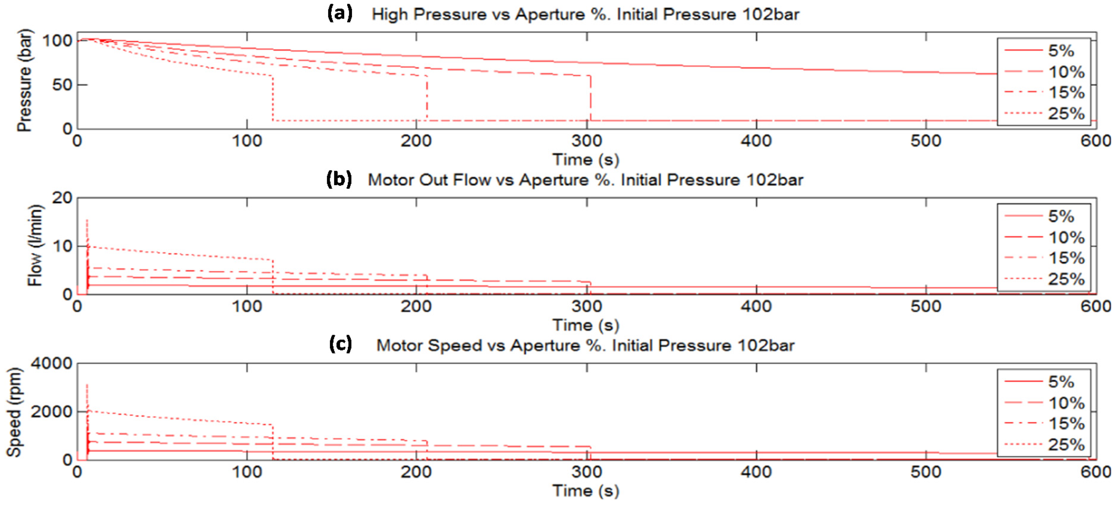
In this case, the ability of the hydraulic motor movement to generate energy is related to the oil volume stored in the HP Accumulator. In Figure 19, the higher the control valve aperture percentage, the lower the autonomy of the volume stored by the HP accumulator.
Figure 19. HP accumulator pressure evolution in bar (a). Hydraulic Motor Flow evolution in L/min (b). Hydraulic Motor Speed in rpm (c). Comparison between different control valve apertures when PTO input movement is blocked.
Energies 08 02230 g019
For the sake of the simulations, results from an initial pressure of 102 bar are shown. The results are independent of the geometrical configuration of the hydraulic cylinders, as there is no movement at the Input of the PTO. The results of last simulation test could be used to implement a strategy to extend the period of continuous rotation of the hydraulic motor and generator group whilst the sea conditions remain calm.

4.2. Experimental Validation and Model Adjustment

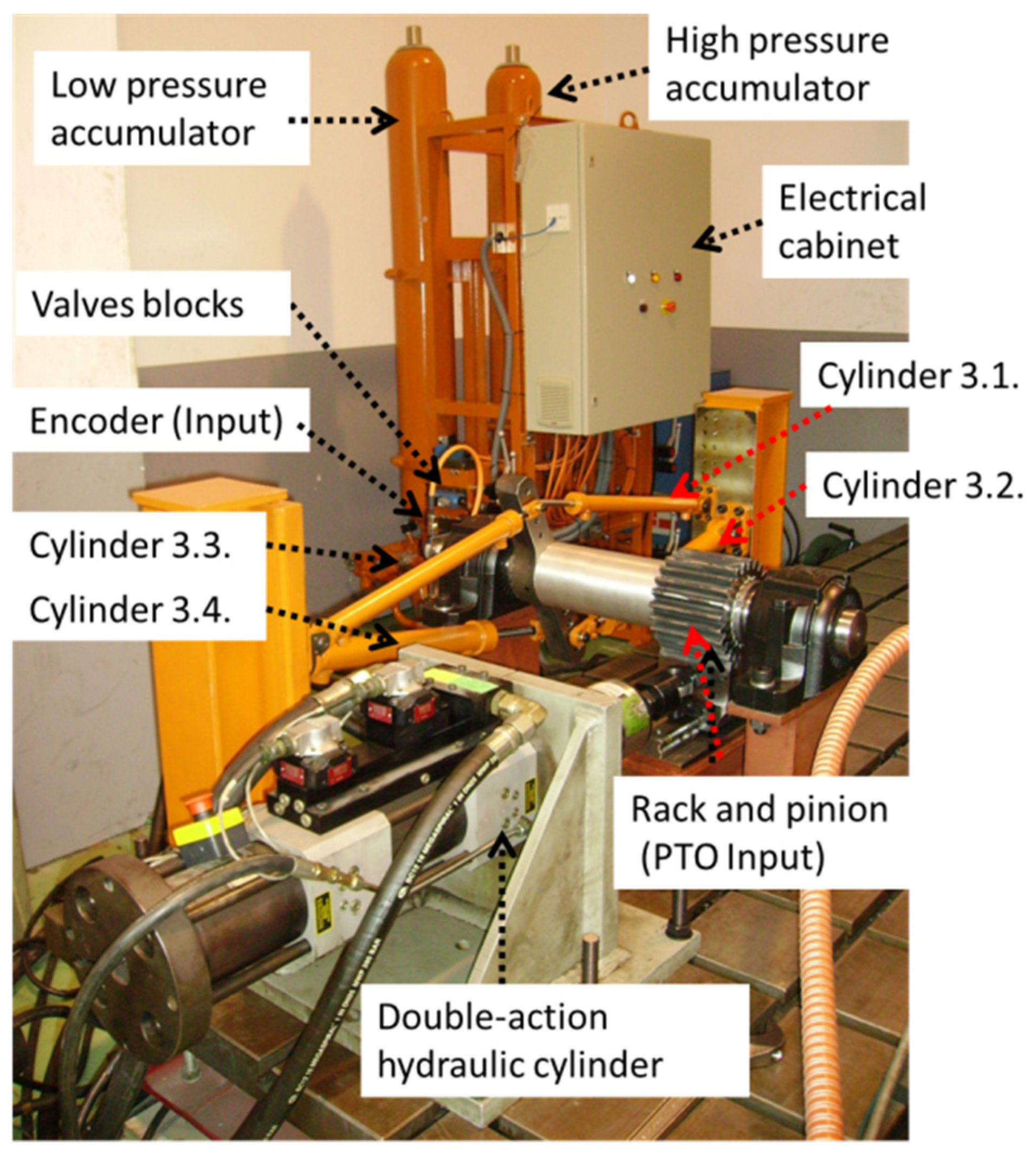
The following methodology has been carried out to perform the adjustment of the dynamic model, once it is optimized. Firstly, the parameters required for the components of the model have been completed using the datasheet of each manufacturer. Secondly, structural stiffness and damping of the mechanical test bench setup have been estimated using finite element software. Thirdly, the open loop behavior of the PTO has been adjusted using the Test bench shown in Figure 20. This experimental evaluation has been carried out using the specific geometrical configuration for hydraulic cylinders, as defined in Config 1.
The objectives of these experimental tests are, firstly, to adjust the relative amount of trapped air inside the Hydraulic Fluid block of the model and, secondly, to define the discharge coefficient and look-up table of the control valve related to the aperture percentage.
To adjust the relative amount of trapped air in the model, experimental values of the high pressure gauge have been collected and compared with simulated values. The experimental evaluation has been performed using different active hydraulic cylinders starting at different initial pressures.
A double-acting hydraulic cylinder controlled by a third-party software has been used for moving the rack-pinion geared system which is defined as the PTO input. The amplitude and the frequency of a sinusoidal signal first have to be defined. A movement of ±40 mm at 0.1 Hz is applied to the rack-pinion geared system charging the HP Accumulator with the control valve closed. This input signal does not exceed the maximum design values of the PTO input, corresponding to an angular displacement of ±30° at low angular speed (0–5 rad/s) [27].
Figure 20. Hydraulic PTO. Main elements of the Test bench. PTO Input.
Energies 08 02230 g020
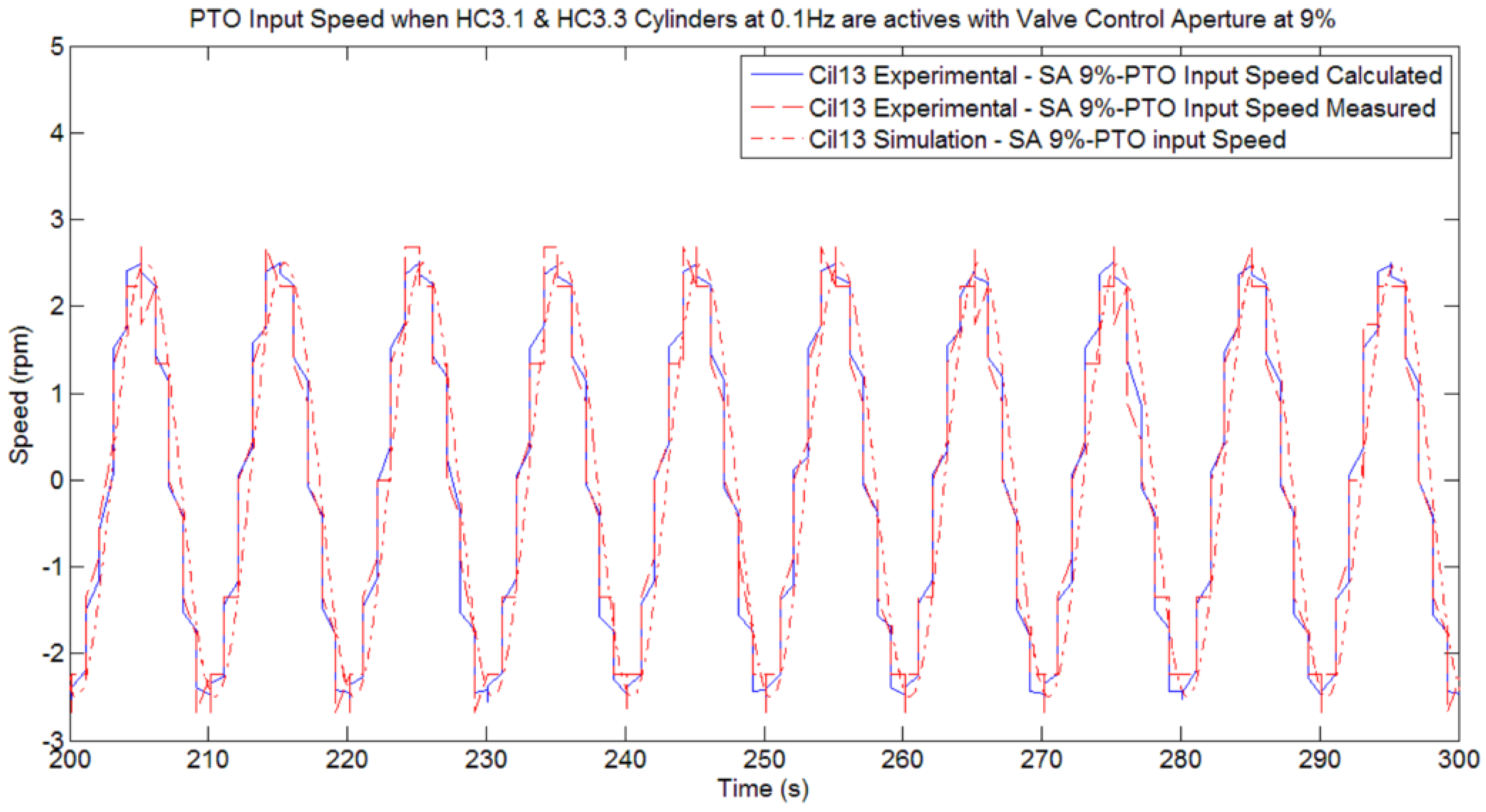
Figure 21 shows the simulated input speed, the on-line calculated input speed and the directly measured input speed obtained by the encoder placed in the Pivoting Axis (PTO input). The maximum input speed is approximately 2.5 rpm. The resolution of the encoder is not high enough to show a steady speed behavior.
Figure 21. Comparison between Simulated PTO Input speed and Calculated/Measured PTO Input speed.
Energies 08 02230 g021
This results in the curves representing the experimental values having a step like shape. This sinusoidal input speed is used in all tests performed to adjust the amount of trapped air, independently of the number of active hydraulic cylinders.
Figure 22, Figure 23, Figure 24 and 
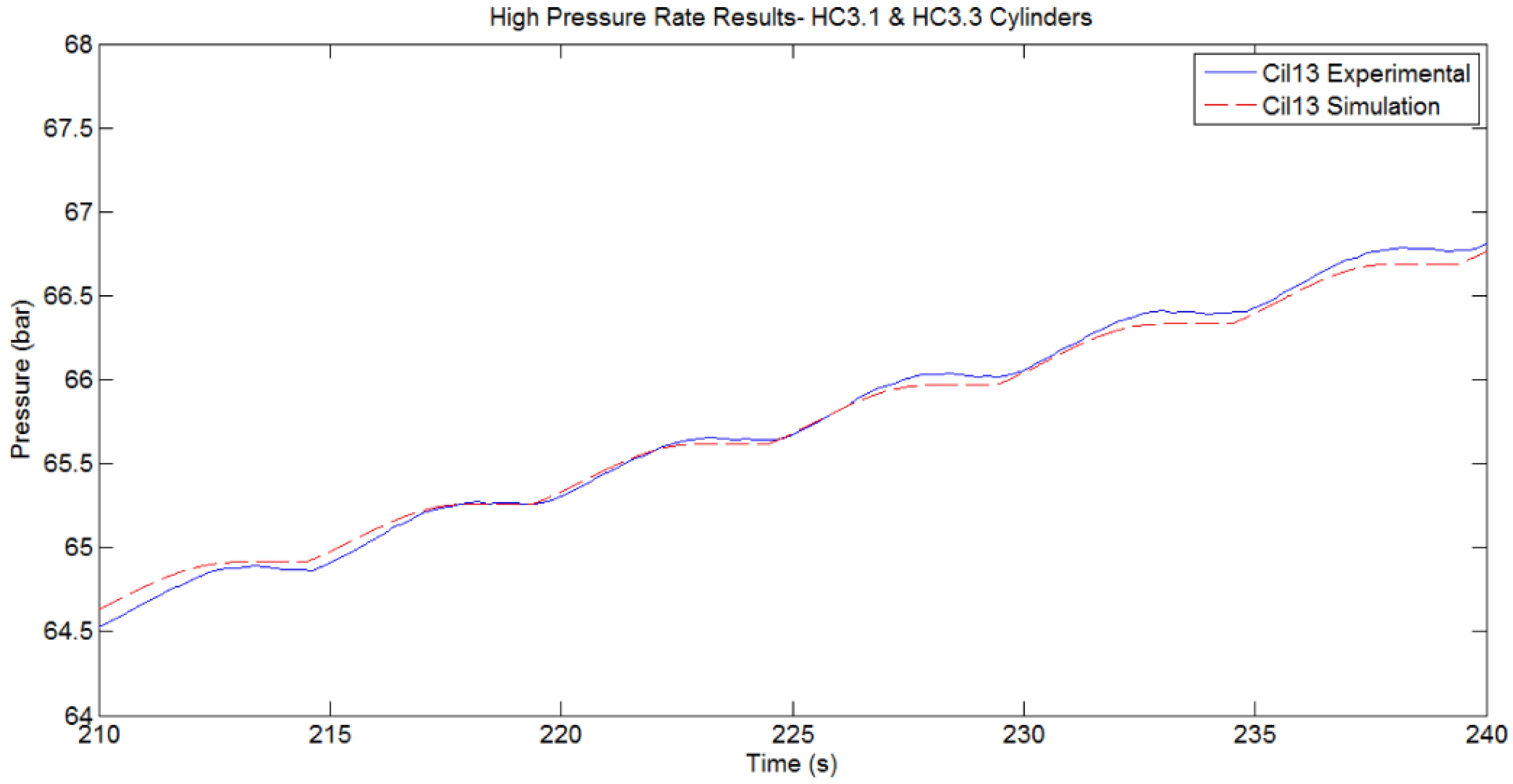
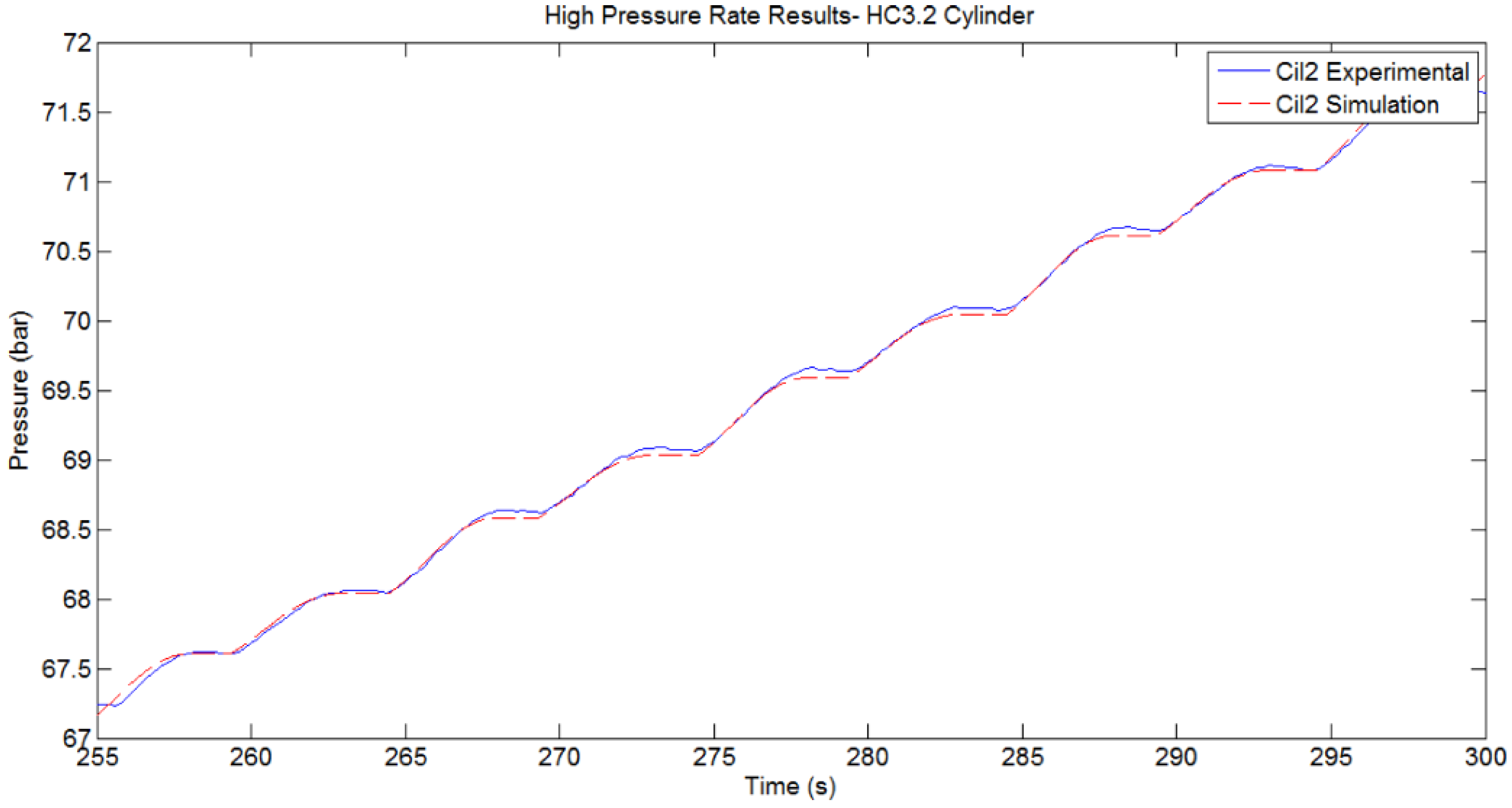
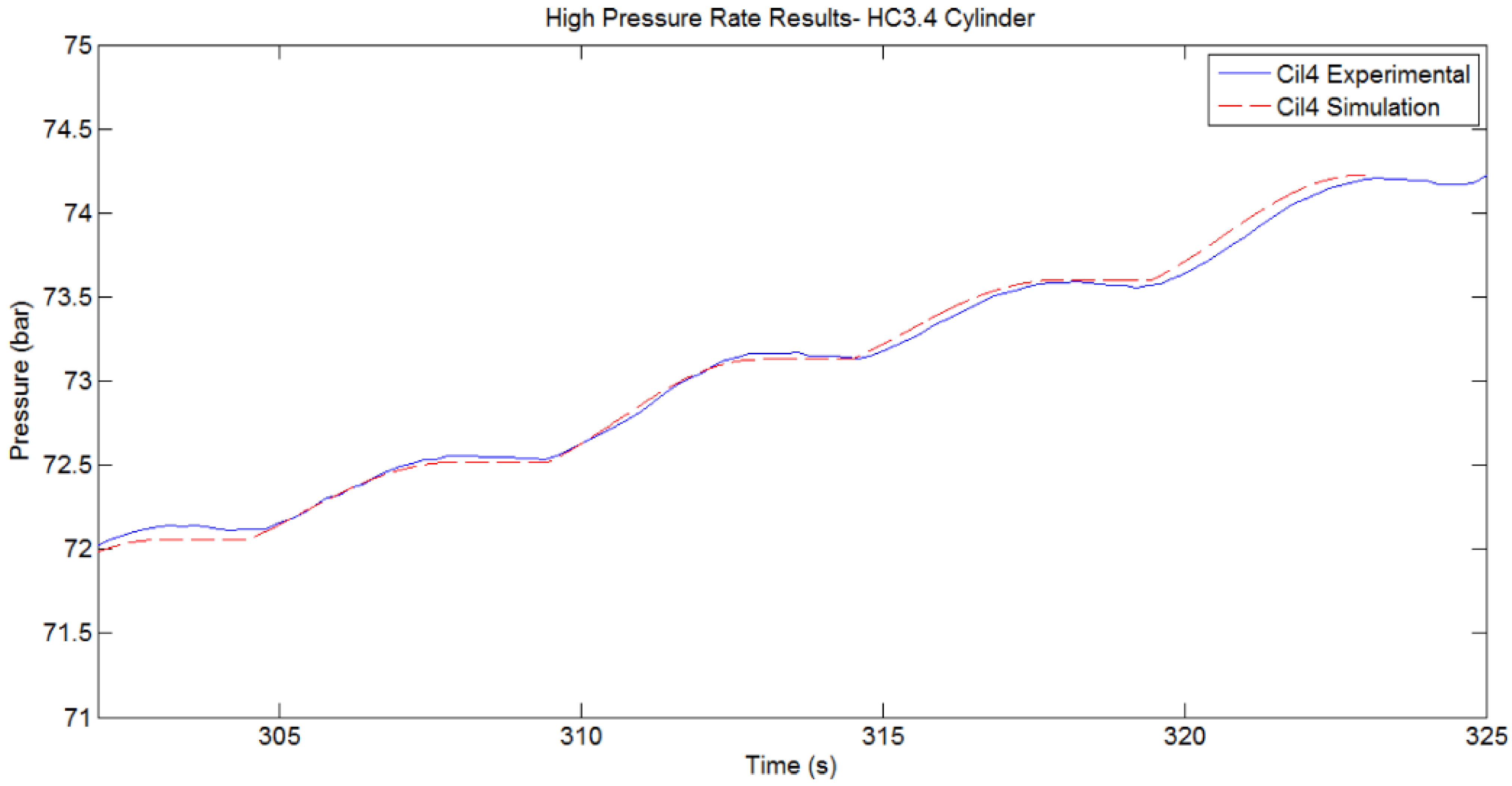
Figure 25 show the evolution of the simulated and experimentally measured pressure of the HP Accumulator after activating different hydraulic cylinders when the amount of trapped air has been adjusted to 6%. In all cases the simulated and experimental signals are very similar.
Figure 22. Comparison between Simulated and Experimentally Measured pressure of HP Accumulator. Active cylinders HC3.1 and HC3.3. Initial Pres. 64.5 bar. Geometrical layout: Config 1.
Energies 08 02230 g022
Figure 23. Comparison between Simulated and Experimentally Measured pressure of HP Accumulator. Active cylinder HC3.2. Initial Pres. 67.2 bar. Geometrical layout: Config 1.
Energies 08 02230 g023
Figure 24. Comparison between Simulated and Experimentally Measured pressure of HP Accumulator. Acitve cylinder HC3.4. Initial Pres. 72 bar. Geometrical layout: Config 1.
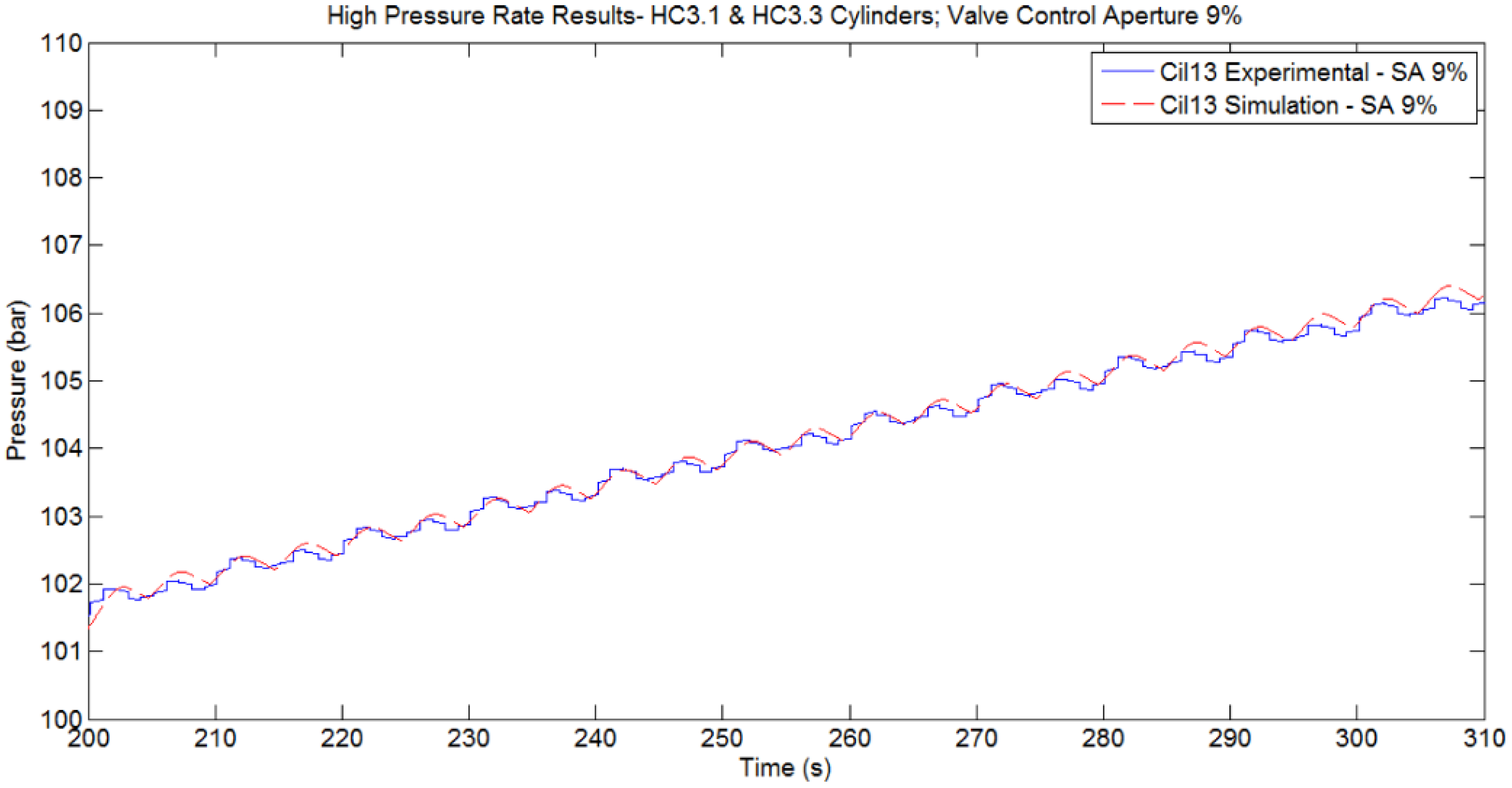
Energies 08 02230 g024
Figure 25. Comparison between Simulated and Experimentally Measured pressure of HP Accumulator. Active cylinders HC3.1 and HC3.3. Valve Control Aperture 9%. Initial Pres. 101.5 bar. Geometrical layout: Config 1.
Energies 08 02230 g025
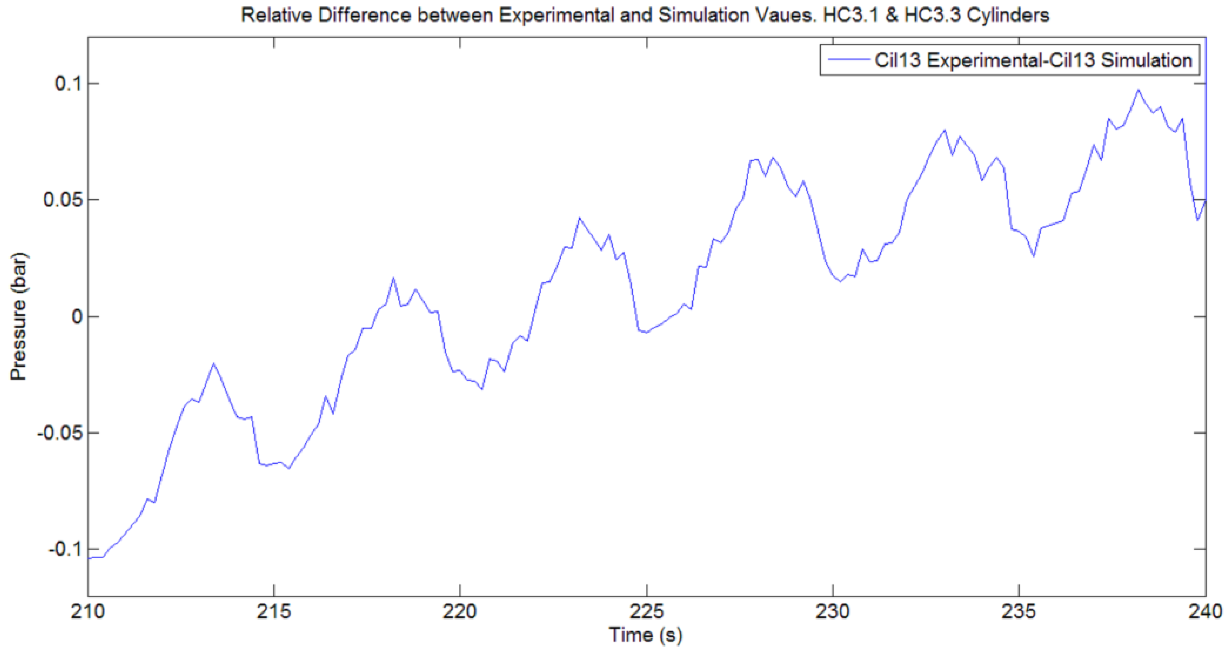
In order to demonstrate that the behavior is reasonably constant independent of the time interval, the following figures use different time intervals. In order to compare between simulated and experimentally measured pressures of HP accumulator, Figure 26 depicts the relative difference between both signals using the experimental values as reference. The relative difference is very low and shows a slight increment with time.
Figure 26. Relative Difference between Experimentally Measured and Simulated pressure of HP Accumulator. Active cylinders HC3.1 and HC3.3. Initial Pres. 64.5 bar. Geometrical layout: Config 1.
Energies 08 02230 g026
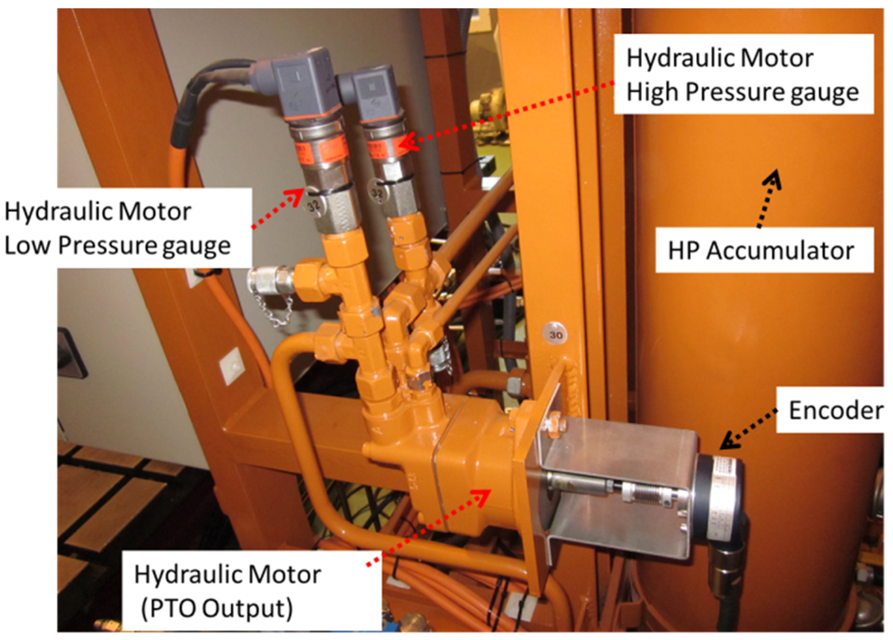
The other experimental tests to be compared with those from the simulations are related to the PTO output and the control valve adjustment. 
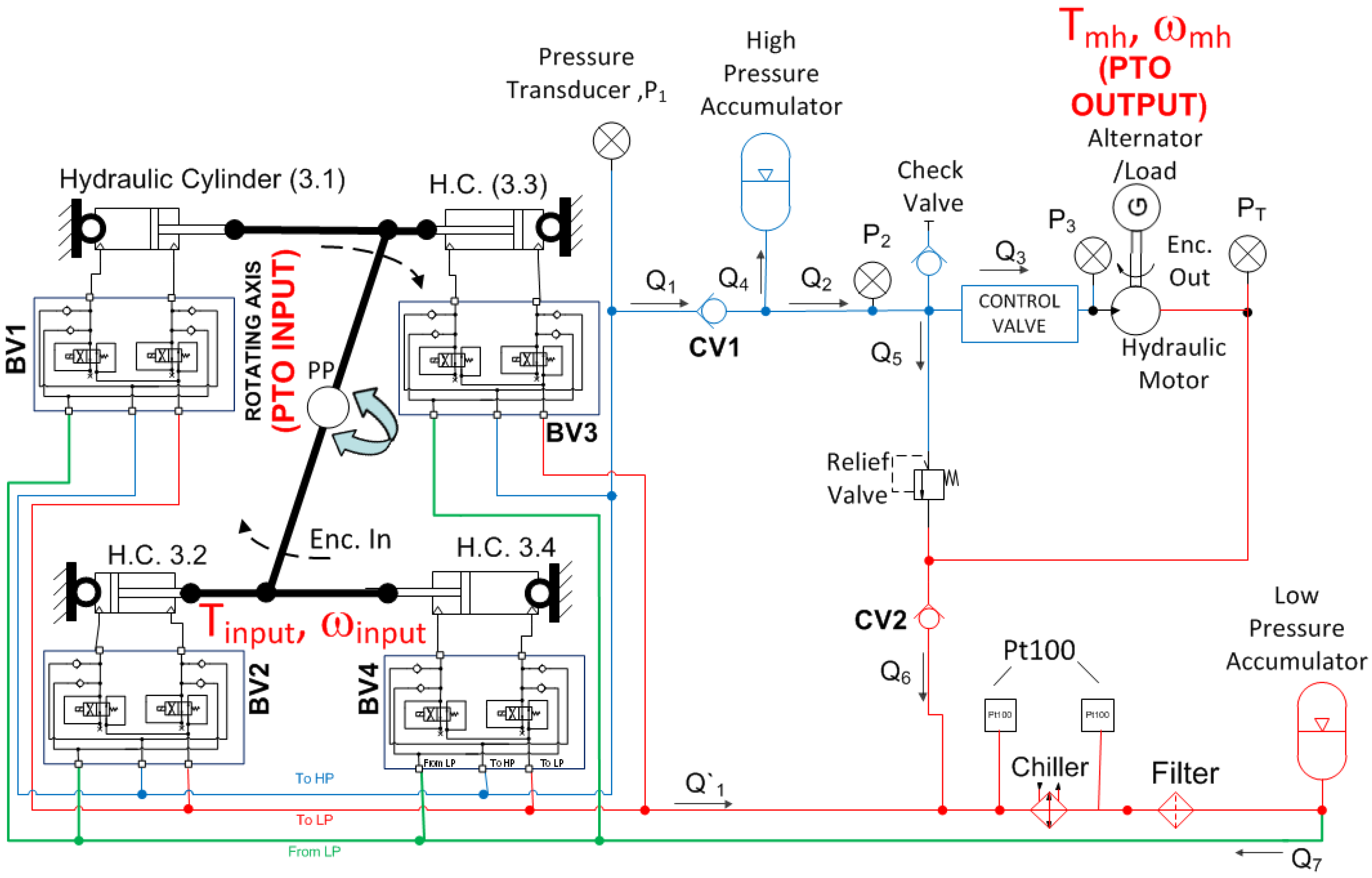
Figure 27 displays the main components of the PTO Output. The objective of these tests is to adjust the behavior of the control valve in order to obtain similar pressure decay in the pressure of the HP Accumulator and a similar output speed for the hydraulic motor (PTO Output).
Figure 27. Hydraulic Motor. PTO Output.
Energies 08 02230 g027
These tests consist of charging the HP Accumulator at a specific pressure. Once the pressure is reached, the PTO input movement is stopped. Afterwards the control valve is opened to a specific aperture percentage and the pressure of the HP pressure and the speed of the hydraulic motor are measured.
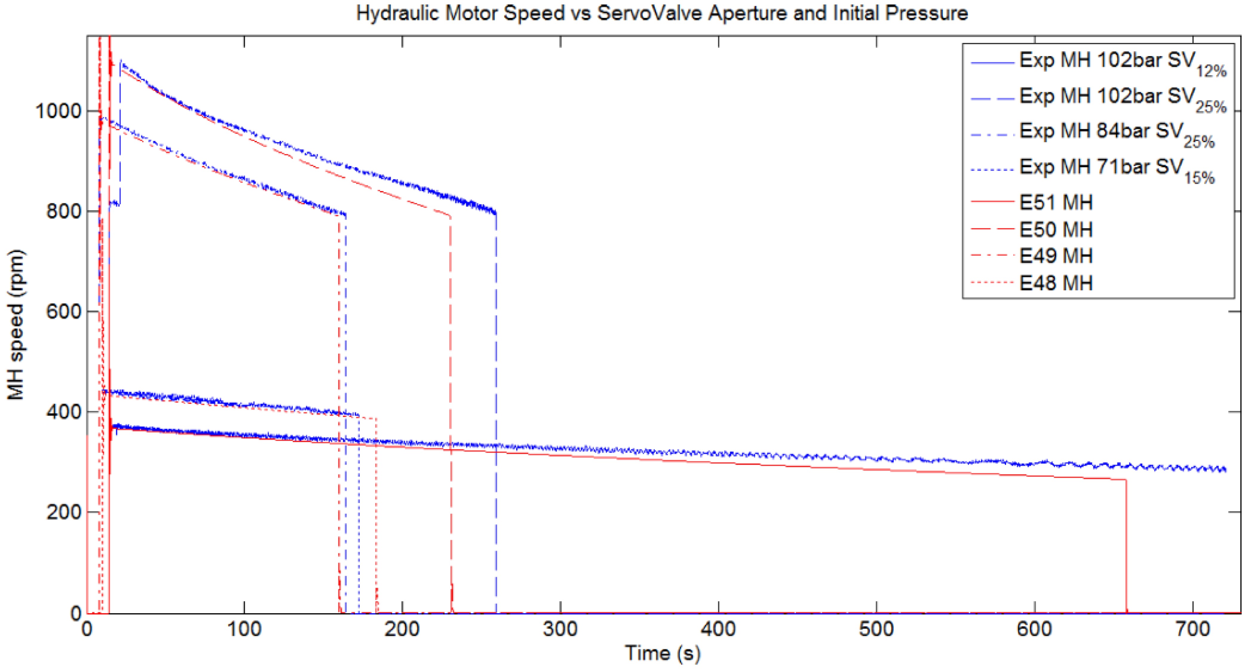
Figure 28 shows the comparison between the simulated and experimental measurements of the hydraulic motor speed (rpm), identified in red and blue respectively. The experimental tests start at different initial pressures (102, 84 and 71 bar) with the control valve opened to different aperture percentages (12%, 15% and 25%). To obtain the results in Figure 28, the control valve has been parameterized with a discharge coefficient of 0.154 and by applying the control valve area versus control valve aperture percentages as identified in Table 11.
Figure 28. PTO Output. Hydraulic motor speed (rpm) comparison between simulated (red) and experimental (blue) tests.
Energies 08 02230 g028
Table 11. Control valve aperture percentage versus control valve area.
Parameter DescriptionValue
Control Valve Aperture (%)[0,10,20,30,40,50,60,70,80,90,100]
Control Valve Area (mm2)[0; 1.136; 2.756; 5.336; 8.876; 13.376; 18.836; 25.256; 32.636; 38.42; 44.18]
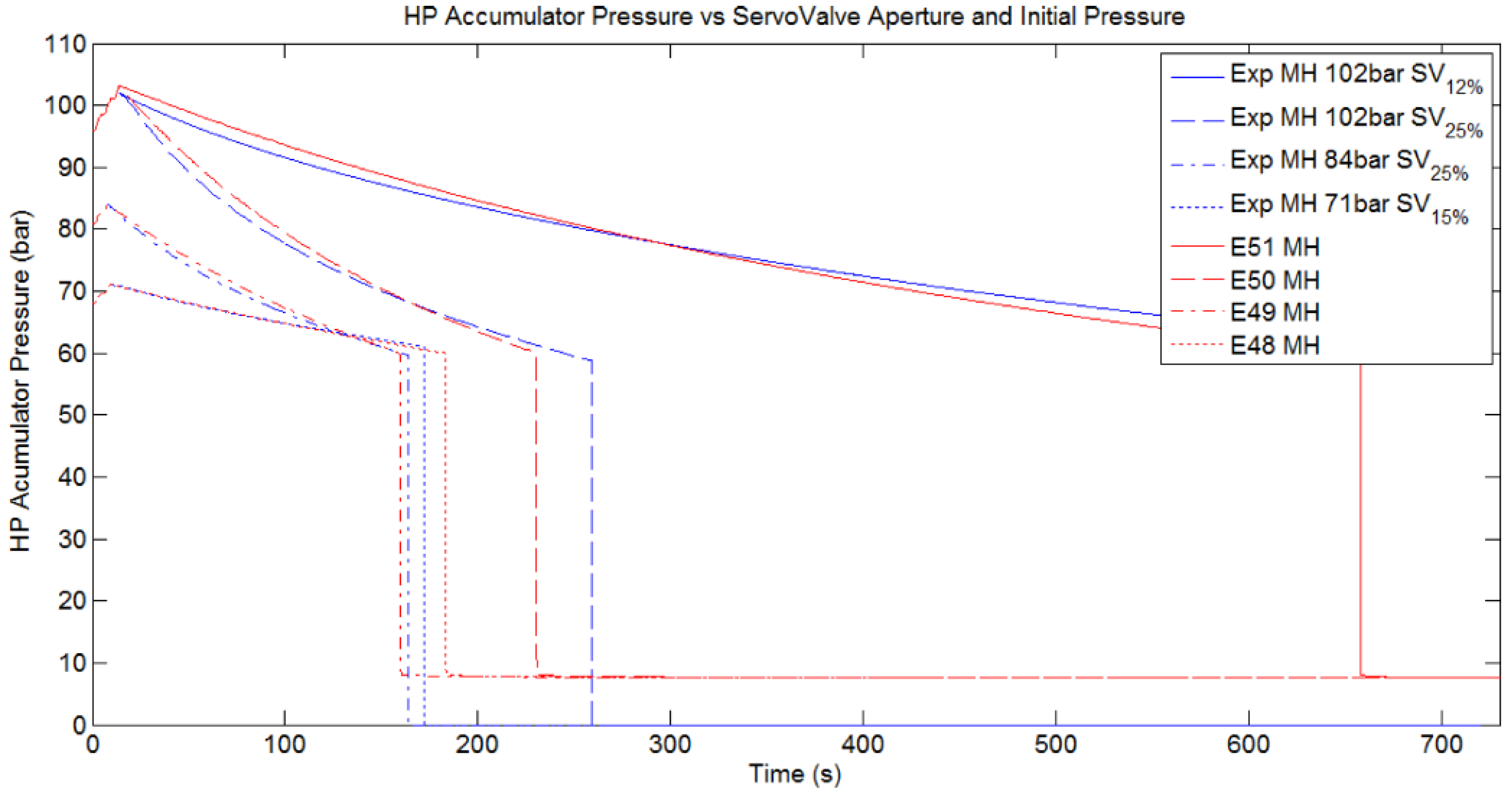
Figure 28 and Figure 29 show a good correlation between the experimental and simulated values in all of the tests, and they relate respectively to the hydraulic motor speed and the HP Accumulator pressure. However, it seems that experimental tests provide more autonomy than in the simulations. This behavior can be justified due to the method used for characterizing the control valve.
The characterization of the control valve has been performed assuming that the control valve allows a specific flow independent of the pressure drop in the control valve. The flow through the control valve also depends on the pressure drop between the inlet and outlet of the valve ports.
Figure 29. PTO Output. HP Accumulator pressure (bar) comparison between simulated (red) and experimental (blue) tests.
Energies 08 02230 g029
A better parameterization for these kind of control valves can be performed using the methods specified by Tchkalov [52]. The transient response of the actuator can be optimized using this method. In addition, it is also possible to include the frequency response characteristics of the valve. However, all these methods are based on the application of optimization procedures with functions from the Optimization Toolbox, which were not available to the author.

4.3. Model Assessment

According to the simulations using the PTO model developed in this work and compared with the experimental values obtained using a test bench, the model is able to follow the expected behavior using a specific sinusoidal input movement applied to a rack-pinion system.
The comparison between simulated and experimental values using the same input signal demonstrates a good correlation between the model and the obtained using the manufactured test bench. Once the model is properly adjusted further investigations will be carried out to study some strategies to control a specific point-absorber using this PTO model as the mean power efficiency is 0.728 [27].

5. Conclusions

This paper fully describes a novel PTO based on a double-acting cylinder array. The system main features provoke a braking torque that can be controlled through the modification of L (AB) and R (OB) geometrical parameters and through the activation of more than one hydraulic cylinder whilst also controlling the system pressure.
The complete model of a PTO based on double-acting cylinders array has been presented, developed using a simulation toolbox based on a port-based approach to model hydraulic systems. The main advantage of this modeling method lies in the ability of easily constructing the required hydraulic model(s). However, the main drawback comes from the ability of the model developer to correctly interpret the datasheet for each hydraulic component with respect to the parameters used by the model. Depending on the manufacturer of the hydraulic components, sometimes they are unavailable, or the available parameters do not correspond to those ones used in the block of the simulation toolbox. The model assumes that the temperature in the hydraulic fluid does not change during the simulation. However, it takes into account several parameters that consider most of the hydraulic losses caused by the hydraulic pipes and components, including real characteristics of the hydraulic fluid.
The paper shows results from simulations of the developed model using four geometrical configurations in conjunction with the application of four different combinations of active hydraulic cylinders. However, this PTO consists of four double-acting hydraulic cylinders and each hydraulic cylinder is able to use up to twenty different possible assembly configurations. In addition, up to nineteen different restraining torques could be applied for each geometrical configuration. This availability and the control of the operating pressure allows the application of a great number of restraining torques.
The simulation results have demonstrated that the defined PTO is able to apply different restraining torques by modifying geometrical characteristics and activating or deactivating hydraulic cylinders depending on the input signal. The modification of the geometrical parameters is related to the modification of the climate conditions, whereas the activation or deactivation of the double-acting hydraulic cylinders could be used to adjust the restraining torque for the current sea state.
In addition, the developed model has been further refined through the comparison between several experimental results performed on a real Test bench and the simulation tests. The adjustment has been performed to obtain a similar high pressure evolution in three different scenarios, valve control completely closed, completely open or open to a given percentages of a fully open aperture. The comparison after the adjustment indicates that the model is accurately tuned. Therefore, this model can be utilized to propose control strategies on specific Wave Energy Converters like point absorbers.
The detailed PTO is flexible enough to be used under different sea conditions by selecting the geometrical parameters (off-line), while the activation and de-activation of the double-acting hydraulic cylinders can be decided by a real-time controller to adjust the restraining torque to the current situation of a given sea state. Taking into account the flexibility of this PTO, the devices for wave energy extraction or WECs can take advantage of the possibility of developing control strategies such as latching, unlatching and variable time-amplitude pulse control.
Future work will focus on the dynamic simulation of a specific WEC using this PTO in order to analyze optimal control algorithms to maximize the power extraction.

Acknowledgments

The authors wish to acknowledge the financial support received from the Spanish Government, by means of the research project subsidy from the PSE-MAR program contract PS-440000-2008-1, “Obtención de Energía de las Olas”. This work was also supported in part by the Regional Government of the Basque Country (Project IT719-13) and UPV/EHU under grant UFI11/28. The authors would like to thank Richard Seddon for his help in reviewing this article.

Author Contributions

Juan Carlos Antolín-Urbaneja is the main researcher who initiated and organized the research reported in the paper. He was involved in each phase of the research activities including the development of the model, the validation of the simulation test and the adjustment of the model with respect to experimental results. Also, as the first author, he was responsible for writing the main parts of the paper, including the state of the art included in the Introduction of the paper. Besides he is a co-author of the patent application of the Power Take-Off system model detailed in the paper. Alain Cortés was involved in the development of the model using MATLAB, Simulink and Simhydraulics code. He participated in the presentation of the results and in the adjustment of the model. Itziar Cabanes was involved in the development of the model and she contributed to writing some parts of the paper. Joseba Lasa and Patxi Estensoro are co-authors in the development of the patent application and they participated in the collection of the experimental results. Due to her long and fruitful experience in the area of modelling and control, Marga Marcos contributed to the paper in the review of the full paper.

Conflicts of Interest

The authors declare no conflict of interest.

References

  1. Salter, S.H.; Taylor, J.R.M.; Caldwell, N.J. Power conversion mechanisms for wave energy. Proc. Inst. Mech. Eng. Part M J. Eng. Marit. Environ. 2002, 216, 1–27. [Google Scholar]
  2. Babarit, A.; Duclos, G.; Clément, A.H. Comparison of latching control strategies for a heaving wave energy device in random sea. Appl. Ocean Res. 2004, 26, 227–238. [Google Scholar] [CrossRef]
  3. Babarit, A.; Guglielmi, M.; Clément, A.H. Declutching control of a wave energy converter. Ocean Eng. 2009, 36, 1015–1024. [Google Scholar] [CrossRef]
  4. Falcão, A.F.D.O. Phase control through load control of oscillating-body wave energy converters with hydraulic PTO system. Ocean Eng. 2008, 35, 358–366. [Google Scholar] [CrossRef]
  5. Falcão, A.F.D.O. Modelling and control of oscillating-body wave energy converters with hydraulic power take-off and gas accumulator. Ocean Eng. 2007, 34, 2021–2032. [Google Scholar] [CrossRef]
  6. Henderson, R. Design, simulation, and testing of a novel hydraulic power take-off system for the Pelamis wave energy converter. Renew. Energy 2006, 31, 271–283. [Google Scholar] [CrossRef]
  7. Plummer, A.R.; Schlotter, M. Investigating the performance of a hydraulic power take-off. In Proceedings of the 8th European Wave and Tidal Energy Conference, Uppsala, Sweden, 7–10 September 2009; pp. 729–735.
  8. Ricci, P.; Lopez, J.; Santos, M.; Ruiz Minguela, P.; Villate, J.L.; Salcedo, F.; Falcão, A.F.D.O. Control Strategies for a Wave Energy Converter Connected to a hydraulic power take-off. IET Renew. Power Gener. 2011, 5, 234–244. [Google Scholar] [CrossRef]
  9. Rhinefrank, K.; Agamloh, E.B.; von Jouanne, A.; Wallace, A.K.; Prudell, J.; Kimble, K.; Aills, J.; Schmidt, E.; Chan, P.; Sweeny, B.; et al. Novel ocean energy permanent magnet linear generator buoy. Renew. Energy 2006, 31, 1279–1298. [Google Scholar] [CrossRef]
  10. Elwood, D.; Schacher, A.; Rhinefrank, K.; Prudell, J.; Yim, S.; Amon, E.; Al, E. Numerical modelling and ocean testing of a direct-drive wave energy device utilizing a permanent magnet linear generator for power take-off. In Proceedings of the 28th International Conference on Ocean Offshore Arctic Engineering, Honolulu, HI, USA, 31 May–5 June 2009; pp. 817–824.
  11. Falcão, A.F.D.O. Wave energy utilization: A review of the technologies. Renew. Sustain. Energy Rev. 2010, 14, 899–918. [Google Scholar] [CrossRef]
  12. Kamizuru, Y.; Verdegem, L.; Erhart, P.; Langenstein, C.; Andren, L.; Lenßen, M. Efficient power take-offs for ocean energy conversion. In Proceedings of the 4th International Conference on Ocean Energy, Dublin, Ireland, 17–19 October 2012; pp. 1–8.
  13. Cummins, W.E. The impulse response function and ship motions. Schiffstechnik 1962, 9, 101–109. [Google Scholar]
  14. Budal, K.; Falnes, J.; Hals, T.; Iversen, L.C.; Onshus, T. Model experiment with a phase controlled point absorber. In Proceedings of the Second International Symposium on Wave and Tidal Energy, BHRA Fluid Engineering, Cambridge, UK, 23–25 September 1981; pp. 191–206.
  15. Falnes, J.; Budal, K. Preliminary Design and Model Test of a Wave-Power Converter: Budal’s 1978 Design Type E; Division of Physics, University of Trondheim: Trondheim, Norway, 1993. [Google Scholar]
  16. Eidsmoen, H. Simulation of Slack-Moored Heaving-Buoy Wave-Energy Converter with Phase Control. Available online: http://folk.ntnu.no/falnes/web_arkiv/InstFysikk/simwec.pdf (accessed on 12 December 2012).
  17. Eidsmoen, H. Simulation of Tight-Moored Amplitude-Limited Heaving-Buoy Wave-Energy Converter with Phase Control. Available online: http://folk.ntnu.no/falnes/web_arkiv/InstFysikk/simconve.pdf. (accessed on 12 December 2012).
  18. Eidsmoen, H. Tight-moored amplitude-limited heaving buoy wave-energy converter with phase control. Appl. Ocean Res. 1998, 20, 157–161. [Google Scholar] [CrossRef]
  19. Josset, C.; Babarit, A.; Clément, A.H. A wave-to-wire model of the SEAREV wave energy converter. Proc. Inst. Mech. Eng. Part M J. Eng. Marit. Environ. 2007, 221, 81–93. [Google Scholar] [CrossRef]
  20. Karnopp, D.C.; Margolis, D.L.; Rosenberg, R.C. System Dynamics: Modelling and Simulation of Mechatronics Systems, 4th ed.; John Wiley & Sons Inc.: Hoboken, NJ, USA, 2006. [Google Scholar]
  21. Engja, H.; Hals, J. Modelling and simulation of sea wave power conversion systems. In Proceedings of the 7th European Wave and Tidal Energy Conference, Oporto, Portugal, 11–14 September 2007.
  22. Bacelli, G.; Gilloteaux, J.C.; Ringwood, J. State space model of a hydraulic power take off unit for wave energy conversion employing bondgraphs. In Proceedings of the World Renewable Energy Conference, Glasgow, Scotland, 19–25 July 2008; pp. 1–4.
  23. Kurniawan, A.; Pedersen, E.; Moan, T. Bond graph modelling of a wave energy conversion system with hydraulic power take-off. Renew. Energy 2012, 38, 234–244. [Google Scholar] [CrossRef]
  24. Cargo, C.; Plummer, A.; Hillis, A.; Schlotter, M. Optimal design of a realistic hydraulic power take-off in irregular waves. In Proceedings of the 9th European Wave and Tidal Energy Conference (EWTEC), Southamptom, UK, 5–9 September 2011.
  25. Yang, L.; Moan, T. Dynamic analysis of wave energy converter by incorporating the effect of hydraulic transmission lines. Ocean Eng. 2011, 38, 1849–1860. [Google Scholar] [CrossRef]
  26. Choi, K.-S.; Yang, D.-S.; Park, S.-Y.; Cho, B.-H. Design and performance test of hydraulic PTO for wave energy converter. Int. J. Precis. Eng. Manuf. 2012, 13, 795–801. [Google Scholar] [CrossRef]
  27. Lasa, J.; Antolin, J.C.; Angulo, C.; Estensoro, P.; Santos, M.; Ricci, P. Design, construction and testing of a hydraulic power take-off for wave energy converters. Energies 2012, 5, 2030–2052. [Google Scholar] [CrossRef] [Green Version]
  28. Costello, R.; Ringwood, J.; Weber, J. Comparison of two alternative hydraulic pto concepts for wave energy conversion. In Proceedings of the 9th European Wave and Tidal Energy Conference, Southamptom, UK, 5–9 September 2011.
  29. Kamizuru, Y.; Fissmann, C.; Murrenhoff, H. Hydrostatic drive trains for wave energy converters: Simulation and experiments for efficient design. In Proceedings of the 10th European Wave and Tidal Energy Conference (EWTEC), Aalborg, Denmark, 2–5 September 2013.
  30. Hedegaard Hansen, A.; Pedersen, H.C. Optimal discrete PTO force for point absorber wave energy converters in regular waves. In Proceedings of the 10th European Wave and Tidal Energy Conference (EWTEC), Aalborg, Denmark, 2–5 September 2013.
  31. Hansen, R.; Kramer, M.; Vidal, E. Discrete displacement hydraulic power take-off system for the wavestar wave energy converter. Energies 2013, 6, 4001–4044. [Google Scholar] [CrossRef]
  32. Pastor, J.; Liu, Y. Power absorption modeling and optimization of a point absorbing wave energy converter using numerical method. J. Energy Resour. Technol. 2014, 136. [Google Scholar] [CrossRef]
  33. Pastor, J.; Liu, Y. Frequency and time domain modeling and power output for a heaving point absorber wave energy converter. Int. J. Energy Environ. Eng. 2014, 5, 1–13. [Google Scholar] [CrossRef]
  34. Babarit, A.; Duclos, G.; Clément, A.H. Benefit of latching control for heaving wave energy device in random sea. In Proceedings of the 13th International Offshore and Polar Engineering Conference ISOPE2003, Honolulu, HI, USA, 25–30 May 2003; Volume 3, pp. 341–348.
  35. Dick, W. Wave Energy Converter. US Patent 7 581 901 (B2), 1 September 2009. [Google Scholar]
  36. Dick, W. A Connector System for a Wave Energy Converter. US Patent 2010/111610 (A1), 6 May 2010. [Google Scholar]
  37. Dick, W.; Villegas, C. A Wave Energy Conversion System. US Patent 2012/139261(A1), 7 June 2012. [Google Scholar]
  38. Steenstrup, P.R.; Hansen, A.; Hansen, K. A Wave Power Apparatus Having a Float, and a Pair of Bearings for Supporting the Arm. WO Patent 2005/038246 (A1), 28 April 2005. [Google Scholar]
  39. Steenstrup, P.R.; Hansen, A.; Hansen, K. Wave Power Apparatus Having a Float and Means for Locking the Float in a Position above the Ocean Surface. US Patent 7,579,704 (B2), 25 August 2009. [Google Scholar]
  40. Koivusaari, R.; Tuokkola, Y.; Järvinen, A.; Liljelund, J.; Höyden, A.; Lainema, M. Production Instalation. WO Patent 2004/097212 (A1), 11 November 2004. [Google Scholar]
  41. Lasa, J.; Antolín, J.C.; Estensoro, P. Power Take-Off Device for Wave Energy Transformation. EP 24466118 A1, 20 June 2012. [Google Scholar]
  42. Babarit, A.; Clément, A.H. Optimal latching control of a wave energy device in regular and irregular waves. Appl. Ocean Res. 2006, 28, 77–91. [Google Scholar] [CrossRef]
  43. Korde, U.A. Latching control of deep water wave energy devices using an active reference. Ocean Eng. 2002, 29, 1343–1355. [Google Scholar] [CrossRef]
  44. Antolín-Urbaneja, J.C.; Lasa, J.; Estensoro, P.; Cabanes, I.; Marcos, M. Innovative hydraulic power take-off construction and performance tests for wave energy conversion. Appl. Mech. Mater. 2013, 432, 316–323. [Google Scholar] [CrossRef]
  45. The Mathworks. SimHydraulics® 1. Reference; The Mathworks Inc.: Natick, MA, USA, 2008. [Google Scholar]
  46. The Mathworks. Check valve. In SimHydraulics® 1. Reference; The Mathworks Inc.: Natick, MA, USA, 2008; pp. 2.92–2.97. [Google Scholar]
  47. Hals, J.; Taghipour, R.; Moan, T. Dynamics of a force-compensated two-body wave energy converter in heave with hydraulic power take-off subject to phase control. In Proceedings of the 7th European Wave and Tidal Energy Conference, Porto, Portugal, 11–14 September 2007; Volume V.
  48. Ricci, P.; Lopez, J.; Santos, M.; Villate, J.L.; Salcedo, F.; Falcão, A.F.D.O. Control strategies for a simple point-absorber connected to a hydraulic power take-off. In Proceedings of 8th European Wave and Tidal Energy Conference, Uppsala, Sweden, 7–10 September 2009.
  49. White, F.M. Fluid Mechanics, 7th ed.; McGraw-Hill: New York, NY, USA, 2011. [Google Scholar]
  50. The Mathworks. Hydraulic motor. In SimHydraulics® 1. Reference; The Mathworks Inc.: Natick, MA, USA, 2008; pp. 2.166–2.170. [Google Scholar]
  51. Eaton Electrohydraulic Controls Proportional Directional Valves with Feedback. Technical Catalogue. Document N, V-VLPO-MC007-E. 2008; 9.
  52. Tchkalov, V.; Miller, S. Parameterization of Directional and Proportional Valves in Simhydraulics; The Mathworks Inc.: Natick, MA, USA, 2014. [Google Scholar]

