Fast Modeling of Large Wave Energy Farms Using Interaction Distance Cut-Off

Abstract

In many wave energy concepts, power output in the MW range requires the simultaneous operation of many wave energy converters. In particular, this is true for small point-absorbers, where a wave energy farm may contain several hundred devices. The total performance of the farm is affected by the hydrodynamic interactions between the individual devices, and reliable tools that can model full farms are needed to study power output and find optimal design parameters. This paper presents a novel method to model the hydrodynamic interactions and power output of very large wave energy farms. The method is based on analytical multiple scattering theory and uses time series of irregular wave amplitudes to compute the instantaneous power of each device. An interaction distance cut-off is introduced to improve the computational cost with acceptable accuracy. As an application of the method, wave energy farms with over 100 devices are studied in the MW range using one month of wave data measured at an off-shore site.

1. Introduction

Several wave energy concepts around the world are currently being deployed, as well as grid-connecting full-scale wave energy converters (WECs). To produce a power of more than a few MW and to enable an even power distribution, most wave energy concepts necessarily include arrays of many absorbing units. In particular, this is true for point-absorber WECs, where buoys, small in relation to the wave length, are forced to oscillate by the surface waves. The oscillatory motion can be converted to electricity by means of various methods, including hydraulic pumps or direct-drive generators. An overview of the different concepts can be found in one of several published comprehensive reviews [1,2,3].

This paper concerns large farms of point-absorbing WECs. The individual devices in a farm are not independent, but will interact with scattered and radiated waves. This affects not only the full performance of the farm to a great extent, but may also influence the surrounding coastal or ocean area by the modified wave field [4].

A large number of numerical studies of wave energy farms have been published over the years. The increase in power production and reduction in power fluctuations as functions of the number of devices in a farm were studied in [5,6,7,8], and the effect on the farm performance of the separating distance between devices has been studied in [8,9,10,11,12]. The global geometry can have a large effect on the power output and the fluctuations in an array. In [13], it was shown that modifications of certain array layouts can increase the power by 5% or lead to a decrease of up to 30% compared to the original layout.

A few experimental results of wave energy farms have been reported. In [14], experiments with 24 WECs at a scale of 1:80 were reported, which showed that the best farm layout was 28% more efficient than the worst configuration and that up to 26% of the energy yield from an equivalent number of isolated WECs may be lost due to interference effects. Physical modeling of 25 small-scale WECs showed that radiated waves could reduce the down wave height by 18% [15]. Experiments with full-scale devices have shown that the power fluctuations of the array reduce with an increased amount of devices, with increased damping and with significant wave height [16].

As the mentioned studies show, a thorough understanding of the farm effects is crucial for designing wave energy farms with high power production, low power fluctuations and no negative environmental impact on the surrounding marine region. Experiments are important to validate the numerical and analytical simulations, but are usually expensive and difficult to implement. For a comprehensive study of all parameters affecting the performance of a farm, we must rely on numerical and analytical modeling of a large number of farm configurations and wave climates.

Most of the reported numerical studies of wave energy farms have focused on comparing small arrays with a few interacting devices [17], and only a few have studied farms with over 30 WECs due to the increasing complexity and computational cost with an increasing number of interacting devices. Straight-forward simulations with established software get too heavy when the number of interacting bodies grows. In certain situations, assumptions, such as the point-absorber or plane-wave approximations, can simplify the calculations and enable simulations of a large number of units, but the reliability of the results is then uncertain.

This paper presents an analytical method for the modeling of large wave energy farms by using an interaction distance cut-off, which makes it possible to determine a range for which the hydrodynamical interactions in a farm should be accounted. For the greatest accuracy, an infinite interaction distance cut-off can be chosen, so that the full hydrodynamical interaction between all devices in a farm is computed; the method is then exact within the limitations of linear potential flow theory. The method of including an interaction distance cut-off was first introduced in [18] and extended to include diffraction in [19]. Here, the method is presented and investigated in detail and used to study large wave energy farms.

The method is valuable, not only for optimizing the design parameters of large-scale wave energy farms, but also sheds light on the relative importance of the effect of radiated and diffracted waves in an array, which is of practical importance for all off-shore structures, including platforms and very large floating structures (VLFSs).

To evaluate the performance of large-scale wave energy, it is not sufficient to compare a few selected sea states or to study parks only in the frequency domain. For example, the actual instantaneous power absorbed and converted to electricity by the farm is needed to study the smoothing of power fluctuations, which is required for large-scale grid connection. Here, farms with over 100 WECs are studied during long time series of real continuous wave data, collected at an off-shore test site in Lysekil, Sweden.

The paper is organized as follows. The analytical model is presented in Section 2.1 and Section 2.2 and the concept of interaction distance cut-off introduced in Section 2.3. The accuracy of the model is evaluated in Section 3.1, and the method is used to study large wave energy farms in Section 3.2.

2. Wave Energy Farm Model

2.1. Multiple Scattering

The multiple scattering method was first presented by Kagemoto and Yue [20], who combined the direct matrix method [21,22] with an iterative multiple scattering method [23] to an exact multiple scattering theory (within the assumption of linearized potential flow). For floating truncated cylinders, the infinite matrices in the solution must be truncated, and the method is semi-exact. The method was later combined with the single-body diffraction solution of [24] in [25] and extended to independent radiation in [26]. Here, the multiple scattering theory is reviewed, and the notation used in the paper is presented. In Section 2.3, the concept of a maximal interaction distance cut-off is presented and combined with the multiple scattering method, which enables faster solutions of the scattering problem in larger arrays.

Consider a wave energy farm with N point-absorbing WECs, labeled by indices $j\in \{1,\cdots ,N\}$, in a fluid domain of uniform depth h. Define global coordinates $\overline{x}=(x,y,z)$ with $z=0$ at the undisturbed free water surface and $z=-h$ at the seabed. Each WEC consists of a direct-driven linear generator at the seabed connected by a stiff wire to a float at the sea surface; see Figure 1. A priori, the floats may be of different shapes and dimensions and move in six degrees of freedom, but for simplicity, we here restricted to cylindrical floats of equal radius R and draft d, moving in heave with independent velocities $V^j$. For clarity, the nomenclature used in the paper is summarized in Table 1.

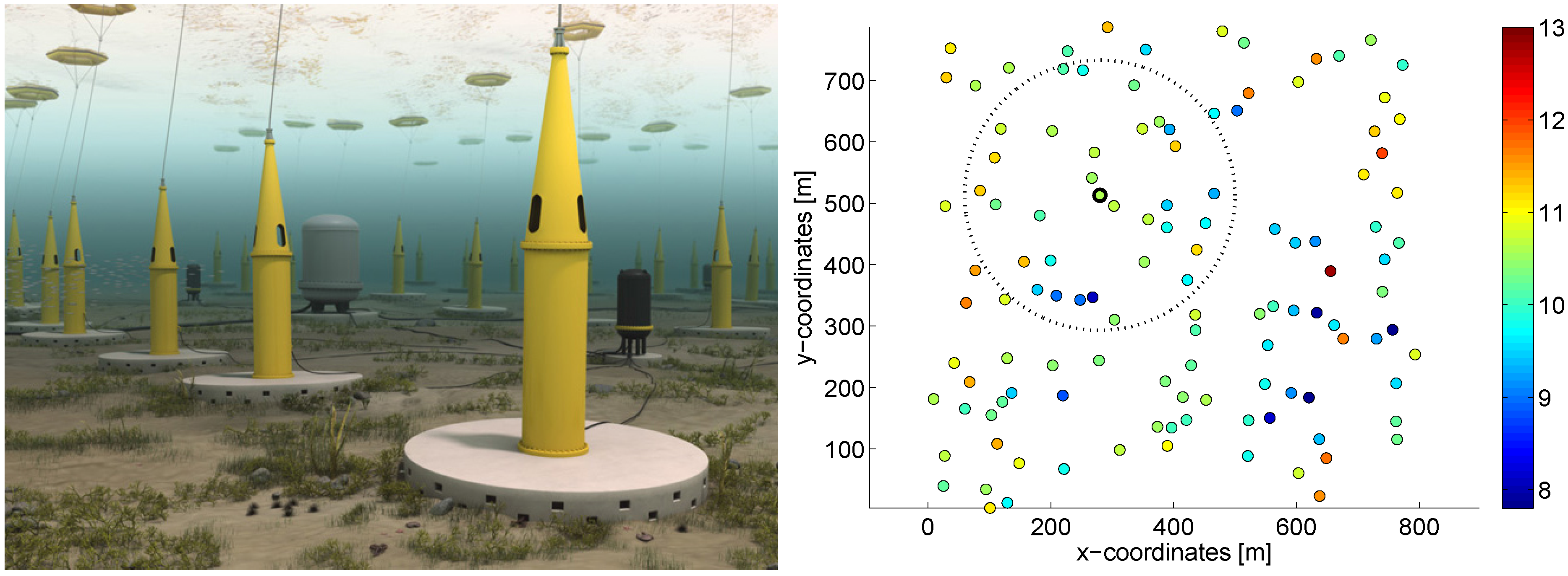
Figure 1. Illustration of a wave energy farm and a simulation of a farm consisting of 120 WECs in a random configuration. The time-averaged power absorption of the individual WECs (kW) is shown with the color bar. The dotted circle illustrates the concept of using interaction distance cut-off in the simulations; in any given array, the hydrodynamical interaction may be computed only between WECs within a specified distance, which speeds up the computations and reduces memory usage, but retains a high accuracy.

Figure 1. Illustration of a wave energy farm and a simulation of a farm consisting of 120 WECs in a random configuration. The time-averaged power absorption of the individual WECs (kW) is shown with the color bar. The dotted circle illustrates the concept of using interaction distance cut-off in the simulations; in any given array, the hydrodynamical interaction may be computed only between WECs within a specified distance, which speeds up the computations and reduces memory usage, but retains a high accuracy.

Table 1. Nomenclature and parameter values, where a numerical value exists.

Parameter and symbol		Value	Parameter and symbol		Value
Incident wave amplitude	A		Velocity of buoys	$V^i$
Incident wave angle	χ		Vertical eigenfunctions	$Z_m\left(z\right)$
Scattering potential	${\varphi }_S$		Bessel functions	$H_n,J_n$
Radiation potential	${\varphi }_R$		Modified Bessel functions	$K_n,I_n$
Coefficients in ${\varphi }_S^{\left(\mathrm{ext}\right)}$	${\alpha }_{mn}^i$		Wave numbers	$k_m$
Coefficients in ${\varphi }_R^{\left(\mathrm{ext}\right)}$	$b_{mn}^i$		Single-body diffr. matrix	$B_{smn}$
Coefficients in ${\varphi }^{\left(\mathrm{int}\right)}$	${\gamma }_{mn}^i$		Separating distance	D
Combined coefficients	${\tilde{\alpha }}_{mn}^i$		Interaction dist.cut-off	$D_{\mathrm{int}}$
Incident wave coefficient	$A_{0n}^i$		Absorbed power	$P^i\left(t\right)$
Angular frequency	ω		Interference factor	q
Number of WECs	N	9–120	Water density	ρ	1025 kg/m
Buoy mass	$m_b$	3.0 tons	Water depth	h	25 m
Translator mass	$m_t$	10.0 tons	Water depth minus draft	L	24.55 m
Power take-off damping	Γ	140 kNs/m	Significant wave height	$H_s$	0.13–5.77 m
Buoy radius	R	3 m	Energy period	$T_e$	2.54–11.3 s
Draft	d	0.45 m	Vertical cut-off	${\Lambda }_z$	20
Gravitational acceleration	g	9.81 m/s${}^2$	Angular cut-off	${\Lambda }_{\theta }$	3

Table 1. Nomenclature and parameter values, where a numerical value exists.

Parameter and symbol		Value	Parameter and symbol		Value
Incident wave amplitude	A		Velocity of buoys	$V^i$
Incident wave angle	χ		Vertical eigenfunctions	$Z_m\left(z\right)$
Scattering potential	${\varphi }_S$		Bessel functions	$H_n,J_n$
Radiation potential	${\varphi }_R$		Modified Bessel functions	$K_n,I_n$
Coefficients in ${\varphi }_S^{\left(\mathrm{ext}\right)}$	${\alpha }_{mn}^i$		Wave numbers	$k_m$
Coefficients in ${\varphi }_R^{\left(\mathrm{ext}\right)}$	$b_{mn}^i$		Single-body diffr. matrix	$B_{smn}$
Coefficients in ${\varphi }^{\left(\mathrm{int}\right)}$	${\gamma }_{mn}^i$		Separating distance	D
Combined coefficients	${\tilde{\alpha }}_{mn}^i$		Interaction dist.cut-off	$D_{\mathrm{int}}$
Incident wave coefficient	$A_{0n}^i$		Absorbed power	$P^i\left(t\right)$
Angular frequency	ω		Interference factor	q
Number of WECs	N	9–120	Water density	ρ	1025 kg/m
Buoy mass	$m_b$	3.0 tons	Water depth	h	25 m
Translator mass	$m_t$	10.0 tons	Water depth minus draft	L	24.55 m
Power take-off damping	Γ	140 kNs/m	Significant wave height	$H_s$	0.13–5.77 m
Buoy radius	R	3 m	Energy period	$T_e$	2.54–11.3 s
Draft	d	0.45 m	Vertical cut-off	${\Lambda }_z$	20
Gravitational acceleration	g	9.81 m/s${}^2$	Angular cut-off	${\Lambda }_{\theta }$	3

Under the assumption of non-viscous, irrotational and incompressible fluid, the governing equation of the fluid velocity reduces to the Laplace equation $\Delta \Phi =0$, where $\Phi (\overline{x},t)$ is the fluid velocity potential. By further assuming non-steep waves, the boundary constraints at the free surface can be linearized, and the total fluid velocity potential will be the superposition of incoming, scattered and radiated waves, $\Phi ={\Phi }_I+{\Phi }_S+{\Phi }_R$. By Fourier transform, the fluid potential can be considered in the frequency domain,

$$\varphi \left(\overline{x}\right)={\int }_{-\infty }^{\infty }\Phi (\overline{x},t)e^{i\omega t}dt$$

(1)

where the frequency dependence in $\varphi \left(\overline{x}\right)$ is implicit.

Define local cylindrical coordinates $(r_j,{\theta }_j,z)$ with origin at the center of each buoy $(x_j,y_j,0)$ and divide the fluid domain into an interior region beneath each buoy, $r_j\le R$, and the exterior region outside, $r_j>R$. By the separation of variables, a general solution to the Laplace equation can be found in terms of eigenfunction expansions. A general outgoing wave in the exterior domain that satisfies the Laplace equation and the boundary constraints at the free surface and seabed takes the form:

$${\varphi }^{j,\mathrm{ext}}=\sum _{n=-\infty }^{\infty }\left[Z_0\left(z\right){\alpha }_{0n}^j\frac{H_n\left(k{r}_j\right)}{H_n\left(kR\right)}+\sum _{m=1}^{\infty }{Z}_m\left(z\right){\alpha }_{mn}^j\frac{K_n\left(k_m{r}_j\right)}{K_n\left(k_{m}R\right)}\right]e^{in{\theta }_j}$$

(2)

where $Z_m\left(z\right)$ are normalized vertical eigenfunctions defined in Equation (A1) in the Appendix and ${\alpha }_{mn}^j$ are unknown coefficients. The wave number $k_0=-ik$ is a solution to the dispersion relation ${\omega }^2=gktanh\left(kh\right)$, and the Hankel functions $H_n\left(k{r}_j\right)$ correspond to propagating modes. The wave numbers $k_m$, $m>0$ are consecutive roots to the dispersion relation ${\omega }^2=-g{k}_{m}tan\left(k_{m}h\right)$, and the Bessel functions $K_n\left(k_m{r}_j\right)$ correspond to evanescent modes. When the outgoing wave corresponds to radiated waves, the coefficients will depend on the oscillation velocities of the buoys $V^j$. To distinguish this case and simplify the expressions, instead of ${\alpha }_{mn}^j$, the notation $V^j{b}_{mn}^j$ will then be used for the coefficients.

A general velocity potential in the interior domain underneath the cylinder that satisfies the Laplace equation and the boundary constraints can be written in the form:

$${\varphi }^{j,\mathrm{int}}=\frac{V^j}{2L^2}({(z+h)}^2-\frac{r^2}{2})+\sum _{n=-\infty }^{\infty }\left[{\gamma }_{0n}^j(\frac{r_j}{R}{)}^{\left|n\right|}+2\sum _{m=1}^{\infty }{\gamma }_{mn}^{j}cos\left({\lambda }_m(z+h)\right)\frac{I_n\left({\lambda }_m{r}_j\right)}{I_n\left({\lambda }_{m}R\right)}\right]e^{in{\theta }_j}$$

(3)

where $I_n\left({\lambda }_m{r}_j\right)$ are modified Bessel functions, ${\lambda }_m=m\pi /L$, and $L=h-d$. If the buoy is stationary, its velocity vanishes $V^j=0$, and the potential only contains the second, homogeneous term.

Consider an incident wave traveling along an angle χ with the x-axis,

$${\varphi }_0=-\frac{igA}{\omega }\frac{cosh\left(k\right(z+h\left)\right)}{cosh\left(kh\right)}{e}^{ik(xcos\chi +ysin\chi )}$$

(4)

where $A=A\left(\omega \right)$ is the amplitude of the waves. In the local coordinates of a buoy, the incident wave can be rewritten using properties of Bessel functions as:

$${\varphi }_0(r_j,{\theta }_j,z)=\sum _{n=-\infty }^{\infty }{A}_{0n}^j{Z}_0\left(z\right)J_n\left(k{r}_j\right)e^{in({\theta }_j-\chi )},A_{0n}^j=-\frac{igA}{\omega Z_0\left(0\right)}{i}^n{e}^{ik(x_{j}cos\chi +y_{j}sin\chi )}$$

(5)

In the most general case, all cylinders are free to oscillate, and there is an incident wave ${\varphi }_0$. The potential in the exterior domain of any buoy will be a superposition of incident wave ${\varphi }_0^i$, scattered and radiated waves ${\varphi }_{S,R}^i$ and incoming waves that are scattered off and radiated from the other buoys ${\varphi }_{S,R}^j$, $j\ne i$,

$${\varphi }^{i,\mathrm{ext}}={\varphi }_0^i+{\varphi }_S^i+{\varphi }_R^i+\sum _{j\ne i}\left({\varphi }_S^j+{\varphi }_R^j\right){|}_i$$

(6)

By using Graf’s addition theorems for Bessel functions, the outgoing waves from one cylinder (Equation (2)) can be written as an incoming wave in the local coordinates of another cylinder as:

$${\varphi }_S^j{|}_i=\sum _{n=-\infty }^{\infty }\left[Z_0\left(z\right)J_n\left(k{r}_i\right)\sum _{l=-\infty }^{\infty }{T}_{0ln}^{ij}{\alpha }_{0l}^j+\sum _{m=1}^{\infty }{Z}_m\left(z\right)\frac{I_n\left(k_m{r}_i\right)}{I_n\left(k_{m}R\right)}\sum _{l=-\infty }^{\infty }{T}_{mln}^{ij}{\alpha }_{ml}^j\right]e^{in{\theta }_i}$$

(7)

where the expressions for $T^{ij}=T_{mln}^{ij}$ are given in the Appendix. Using this expression, the most general diffracted wave in the exterior domain (Equation (6)) takes the form:

$$\begin{array}{cc}\hfill {\varphi }^{i,\mathrm{ext}}& =\sum _{n=-\infty }^{\infty }\left[Z_0\left(z\right)\left(\frac{H_n\left(k{r}_i\right)}{H_n\left(kR\right)}{\tilde{\alpha }}_{0n}^i+J_n\left(k{r}_i\right)(A_{0n}^i+\sum _{l=-\infty }^{\infty }{T}_{0ln}^{ij}{\tilde{\alpha }}_{0l}^j)\right)\right.\hfill \\ & \phantom{=}\left.+\sum _{m=1}^{\infty }{Z}_m\left(z\right)\left(\frac{K_n\left(k_m{r}_i\right)}{K_n\left(k_{m}R\right)}{\tilde{\alpha }}_{mn}^i+\frac{I_n\left(k_m{r}_i\right)}{I_n\left(k_{m}R\right)}\sum _{l=-\infty }^{\infty }{T}_{mln}^{ij}{\tilde{\alpha }}_{ml}^j\right)\right]e^{in{\theta }_i}\hfill \end{array}$$

(8)

where ${\tilde{\alpha }}^i={\alpha }^i+V^i{b}^i$ is the combined coefficient of the scattered and radiated waves.

Continuity between the interior (Equation (3)) and exterior solutions (Equation (8)) and their derivatives along the boundary $r=R$ between the interior and exterior domains imply the infinite system of equations:

$$\sum _{m=0}^{\infty }{D}_{smn}{\tilde{\alpha }}_{mn}^i=-\sum _{m=0}^{\infty }{\tilde{D}}_{smn}\left(A_{0n}^i{\delta }_{m0}+\sum _{j\ne i}\sum _{l=-\infty }^{\infty }{T}_{mln}^{ij}{\tilde{\alpha }}_{ml}^j\right)-V^i{R}_s{\delta }_{n0}$$

(9)

together with an expression for the coefficients γ in the interior solution in terms of the coefficients $\tilde{\alpha }$. The matrices $D_{smn}$ and $R_s$ and their components are defined in the Appendix.

To solve for the unknown coefficients $\tilde{\alpha }$ in Equation (9), we truncate the indices $l,n$ corresponding to the summation over the angular eigenfunctions $e^{in{\theta }_i}$ at ${\Lambda }_{\theta }$ and the indices $m,s$ corresponding to the summation over the vertical eigenfunctions at ${\Lambda }_z$. The solution now becomes semi-analytical, with the finite system of linear equations:

$$[{\tilde{\alpha }}_{sn}^i{]}^s=[B_{smn}{]}_{\phantom{s}m}^s[A_{0n}^i{\delta }_{m0}+\sum _{j\ne i}\sum _{l=-{\Lambda }_{\theta }}^{{\Lambda }_{\theta }}{T}_{mln}^{ij}{\tilde{\alpha }}_{ml}^j{]}^m-[D_{smn}^{-1}{]}_{\phantom{s}m}^s[V^i{R}_m{\delta }_{n0}{]}^m$$

(10)

The single-body diffraction matrix $[B_{smn}]=-[D_{smn}^{-1}][{\tilde{D}}_{smn}]$ will simply be denoted B in what follows. The N equations in Equation (10) can now be combined into a single matrix equation as:

$$\left[\mathrm{DiffMatrix}\right]\left[\tilde{\alpha }\right]=\left[BA\right]+\left[D^{-1}R\right]$$

(11)

where the three vectors $\left[\tilde{\alpha }\right]=[{\tilde{\alpha }}_{mn}^1,\cdots ,{\tilde{\alpha }}_{mn}^N{]}^t$, $\left[BA\right]=[B{A}_{0n}^1,\cdots ,B{A}_{0n}^N{]}^t$ and $\left[D^{-1}R\right]=[D^{-1}{V}^1{R}_m{\delta }_{n0},\cdots ,D^{-1}{V}^N{R}_m{\delta }_{n0}{]}^t$ are of length $N({\Lambda }_z+1)(2{\Lambda }_{\theta }+1)$, and the diffraction matrix is a square matrix of the form:

$$\mathrm{DiffMatrix}=\left(\begin{array}{ccccc}\mathbf{1}& -B{T}^{12}& -B{T}^{13}& \cdots & -B{T}^{1,N}\\ -B{T}^{21}& \mathbf{1}& -B{T}^{23}& \cdots & -B{T}^{2,N}\\ ⋮& ⋮& \ddots & \cdots & ⋮\\ -B{T}^{N,1}& -B{T}^{N,2}& -B{T}^{N,3}& \cdots & \mathbf{1}\end{array}\right)$$

(12)

where each submatrix is a square of size $({\Lambda }_z+1)(2{\Lambda }_{\theta }+1)$.

Solving the multiple scattering problem now amounts to solving for the unknown coefficients $\tilde{\alpha }$ in Equation (11) by computing the inverse of the diffraction matrix. This is the most computationally-demanding task of the problem and is the problem that has been addressed in Section 2.3 by introducing a maximal interaction distance cut-off.

With the coefficients $\tilde{\alpha }$ determined, the fluid velocity potentials in the exterior and interior domains of each buoy are determined, and the dynamical forces can be computed as described in Section 2.2.

Due to the linearity of the problem, the scattering and radiation problem can be solved independently. The scattering problem is the solution to the wave scattering of incident waves among fixed cylinders, i.e., all $V^j=0$. The radiation problem corresponds to the case when all cylinders are free to move, but there is no incident wave, $A_{0n}^i=0$. In both cases, the (incident and radiated) waves will be scattered in the array, and the solution is found by solving the matrix equation (Equation (11)).

2.2. Dynamical Forces and Power Absorption

Once the fluid velocity potentials have been obtained, the dynamical forces can be readily obtained as surface integrals over the wetted surfaces of the buoys, $\overline{F}={\int \int }_{S}pd\overline{S}$. In the heave direction and in the frequency domain, this corresponds to:

$$\begin{array}{cc}\hfill F^i& =i\omega \rho {\int }_{\theta =0}^{2\pi }d\theta {\int }_{r=0}^{R}rdr{\varphi }^{i\left(\mathrm{int}\right)}(r_i,{\theta }_i,-d)\hfill \\ & =\pi i\omega \rho \left[\frac{V^i}{2}(R^2-\frac{R^4}{4})+{\gamma }_{00}^i{R}^2+4R\sum _{m=1}^{\infty }{\gamma }_{m0}^i\frac{{(-1)}^m}{{\lambda }_m}\frac{I_1\left({\lambda }_{m}R\right)}{I_0\left({\lambda }_{m}R\right)}\right]\hfill \end{array}$$

(13)

where the coefficients ${\gamma }_{m0}^i$ are determined from the expression in Equation (A4) in the Appendix.

The heave excitation force corresponds to the case when the buoys are stationary and subject to an incident wave, i.e., $V^i=0$ in Equations (10)–(11). The radiation force corresponds to the case when there is no incident wave, i.e., $A_{0n}^i=0$ in the same equations.

The dynamics of each WEC is determined by a coupled system of equations between the buoy and the translator in the generator. Under the assumption of a stiff connection line between the buoy and the translator, the two equations can be combined into one and take the following form in the time domain:

$$(m_b+m_t){\ddot{z}}^i\left(t\right)=F_{\mathrm{exc}}^i\left(t\right)+F_{\mathrm{rad}}^i\left(t\right)-\Gamma {\dot{z}}^i\left(t\right)+\rho g\pi R^2{z}^i\left(t\right)$$

(14)

where $z^i\left(t\right)$ is the vertical position of the buoy, ρ is the water density and $m_b$, $m_t$ are the masses of the buoy and translator, respectively. The power take-off damping of the generator is modeled here by a constant coefficient Γ. The radiation force can be divided into one part proportional to the velocity of the buoy and one part proportional to the acceleration, $F_{\mathrm{rad}}\left(t\right)=-m_{\mathrm{add}}\ddot{z}-B\dot{z}$, where $m_{\mathrm{add}}$ and B are the added mass and radiation damping. In the frequency domain, this corresponds to $F_{\mathrm{rad}}\left(\omega \right)=[{\omega }^2{m}_{\mathrm{add}}\left(\omega \right)+i\omega B\left(\omega \right)]z\left(\omega \right)$.

The excitation force in the frequency domain is given by the expression in Equation (13), with all buoys stationary, $V^i=0$. Implicit in this expression is the product with the frequency domain amplitude $A^i\left(\omega \right)$ of the incident waves, and we can write $F_{\mathrm{exc}}^i\left(\omega \right)=A^i\left(\omega \right)f_{\mathrm{exc}}^i\left(\omega \right)$ where $f_{\mathrm{exc}}^i\left(\omega \right)$ is the amplitude independent part of the expression.

The equations of motion in the frequency domain then take the form:

$$\left[-{\omega }^2(m_b+m_t+m_{\mathrm{add}}^i\left(\omega \right))-i\omega (B^i\left(\omega \right)+\Gamma )-\rho g\pi R^2\right]z^i\left(\omega \right)=A^i\left(\omega \right)f_{\mathrm{exc}}^i\left(\omega \right)$$

(15)

or equivalently, $z^i\left(\omega \right)=A^i\left(\omega \right)H^i\left(\omega \right)$, where we defined a transfer function $H^i\left(\omega \right)$. By computing the inverse Fourier transform $z^i\left(t\right)=\widehat{z^i\left(\omega \right)}$, the position of the buoy in the time domain can be obtained.

With the position of the buoy determined, the absorbed wave power at any time instant can now be computed as $P^i\left(t\right)=\Gamma {\left({\dot{z}}^i\left(t\right)\right)}^2$. The instantaneous power absorbed by the full farm is then given by the sum:

$$P_{\mathrm{total}}\left(t\right)=\sum _{j=1}^N{P}^j\left(t\right)$$

(16)

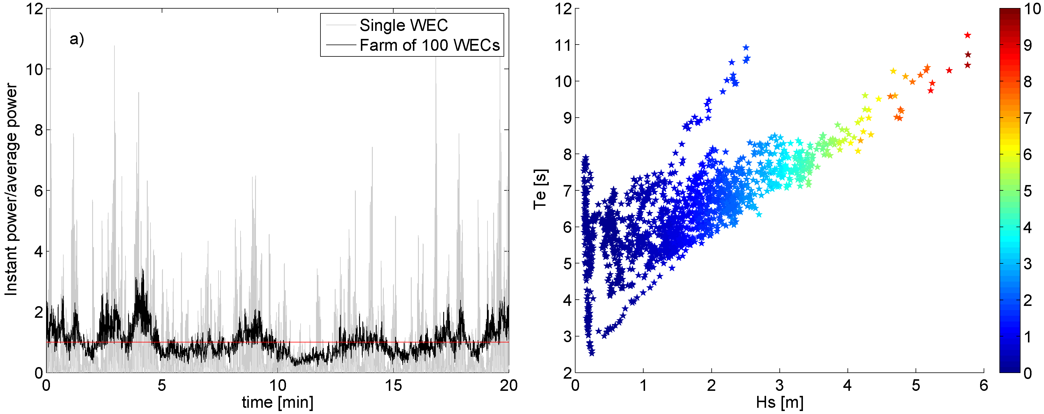
The time series of wave data are collected in sea states of 30 min, each characterized by significant wave height $H_s$ and energy period $T_e$. The absorbed power for single devices and the full farm that is computed in Section 3 is the time-averaged power absorbed during each sea state.

The wave power transported per unit width of the wave front can be written in terms of the significant wave height and energy period by $J=(\rho g^2/64\pi )H_s^2{T}_e$. This is an approximation that might underestimate the wave energy in shallow waters, but is sufficiently accurate for the system studied in this paper [27]. The wave energy incident onto a buoy of radius R is thus $2R\times J$. The capture width ratio (CWR) reflects how much of the wave power is incident on the device that is absorbed [28],

$$\mathrm{CWR}=\frac{\overline{P}}{2R\times J}$$

(17)

where the bar denotes the time-averaged value of the absorbed power. The capture width ratio is often used to compare the absorption and efficiency of different wave energy devices.

2.3. Interaction Distance Cut-Off

As discussed in Section 2.1, the most computationally-extensive part of solving the multiple scattering problem is to solve for the unknown coefficients in Equation (11) by inverting the diffraction matrix. The off-diagonal matrices $B{T}^{ij}$ in the diffraction matrix in Equation (12) contain all of the diffraction coupling terms between the WECs $i,j\in \{1,\cdots ,N\}$. Each of these submatrices are square matrices of the size $({\Lambda }_z+1)(2{\Lambda }_{\theta }+1)$, and the full diffraction matrix is hence a square matrix of size $N({\Lambda }_z+1)(2{\Lambda }_{\theta }+1)$. When computing multiple scattering between all devices in an array, all of these matrices are non-zero, and the diffraction matrix takes the form:

$$\left(\begin{array}{cccccccccccccccccccc}\mathbf{1}& *& *& *& *& *& *& *& *& *& *& *& *& *& *& *& *& *& *& *\\ *& \mathbf{1}& *& *& *& *& *& *& *& *& *& *& *& *& *& *& *& *& *& *\\ *& *& \mathbf{1}& *& *& *& *& *& *& *& *& *& *& *& *& *& *& *& *& *\\ *& *& *& \mathbf{1}& *& *& *& *& *& *& *& *& *& *& *& *& *& *& *& *\\ *& *& *& *& \mathbf{1}& *& *& *& *& *& *& *& *& *& *& *& *& *& *& *\\ *& *& *& *& *& \mathbf{1}& *& *& *& *& *& *& *& *& *& *& *& *& *& *\\ *& *& *& *& *& *& \mathbf{1}& *& *& *& *& *& *& *& *& *& *& *& *& *\\ *& *& *& *& *& *& *& \mathbf{1}& *& *& *& *& *& *& *& *& *& *& *& *\\ *& *& *& *& *& *& *& *& \mathbf{1}& *& *& *& *& *& *& *& *& *& *& *\\ *& *& *& *& *& *& *& *& *& \mathbf{1}& *& *& *& *& *& *& *& *& *& *\\ *& *& *& *& *& *& *& *& *& *& \mathbf{1}& *& *& *& *& *& *& *& *& *\\ *& *& *& *& *& *& *& *& *& *& *& \mathbf{1}& *& *& *& *& *& *& *& *\\ *& *& *& *& *& *& *& *& *& *& *& *& \mathbf{1}& *& *& *& *& *& *& *\\ *& *& *& *& *& *& *& *& *& *& *& *& *& \mathbf{1}& *& *& *& *& *& *\\ *& *& *& *& *& *& *& *& *& *& *& *& *& *& \mathbf{1}& *& *& *& *& *\\ *& *& *& *& *& *& *& *& *& *& *& *& *& *& *& \mathbf{1}& *& *& *& *\\ *& *& *& *& *& *& *& *& *& *& *& *& *& *& *& *& \mathbf{1}& *& *& *\\ *& *& *& *& *& *& *& *& *& *& *& *& *& *& *& *& *& \mathbf{1}& *& *\\ *& *& *& *& *& *& *& *& *& *& *& *& *& *& *& *& *& *& \mathbf{1}& *\\ *& *& *& *& *& *& *& *& *& *& *& *& *& *& *& *& *& *& *& \mathbf{1}\end{array}\right)$$

(18)

where all of the asterisks represent matrices $B{T}^{ij}$ and $\mathbf{1}$ are identity matrices. The matrix in this example corresponds to an array with 20 devices. To solve the multiple scattering problem, this diffraction matrix must be inverted, which poses a very challenging computational task as the array size increases.

We now introduce the notion of interaction distance cut-off $D_{\mathrm{int}}$. For a given wave energy farm, a maximal distance is specified, and coupling terms $B{T}^{ij}$ are only included in the diffraction matrix if they are closer to each other than the specified interaction distance cut-off. That is, only coupling terms between devices that are “close” are included in the diffraction matrix. For large arrays, this will result in a diffraction matrix that is sparse. For example, the above matrix may take the form:

$$\left(\begin{array}{cccccccccccccccccccc}\mathbf{1}& *& & & & & *& & & & *& & & & & & & & *& \\ *& \mathbf{1}& & & *& & & *& & & & & & & & & & & & \\ & & \mathbf{1}& & & & & *& & & & & & *& *& & & & & \\ & & & \mathbf{1}& & & & & & & & & & & & & *& & & *\\ & *& & & \mathbf{1}& & & & *& & & & & & & & & & & *\\ & & & & & \mathbf{1}& & & & *& *& & & *& & & & *& & \\ *& & & & & & \mathbf{1}& & & *& & & *& & & & & & & \\ & *& *& & & & & \mathbf{1}& & & & *& & & & *& & & & \\ & & & & *& & & & \mathbf{1}& *& & & & & *& & & & & \\ & & & & & *& *& & *& \mathbf{1}& & & & & & & & & & \\ *& & & & & *& & & & & \mathbf{1}& & & & & & & & & \\ & & & & & & & *& & & & \mathbf{1}& *& *& & & & & & \\ & & & & & & *& & & & & *& \mathbf{1}& & *& & *& & & \\ & & *& & & *& & & & & & *& & \mathbf{1}& *& & & & & \\ & & *& & & & & & *& & & & *& *& \mathbf{1}& & & & & \\ & & & & & & & *& & & & & & & & \mathbf{1}& & *& *& \\ & & & *& & & & & & & & & *& & & & \mathbf{1}& & & *\\ & & & & & *& & & & & & & & & & *& & \mathbf{1}& *& \\ *& & & & & & & & & & & & & & & *& & *& \mathbf{1}& \\ & & & *& *& & & & & & & & & & & & *& & & \mathbf{1}\end{array}\right)$$

(19)

where only the non-zero submatrices have been included. Various numerical methods can be applied to compute the inverse of sparse matrices, and the computational cost is reduced significantly. For even larger arrays, this reduction in computational cost and memory usage enables the modeling of large farms, which would not be possible for full, dense diffraction matrices.

Since the method with the interaction distance cut-off neglects only coupling terms between devices that are far away from each other in the farm, one can expect that the final result will not be affected to a large extent. This conjecture will be investigated and confirmed in Section 3.

The interaction distance cut-off can be set to any arbitrary distance; it may include only nearest neighbor interactions, or interactions between all devices within a specified distance, or all devices in the farm. No assumptions have to be made on the configuration of the array, on different length scales or equally-spaced WECs.

This paper focuses on arrays of small point-absorber WECs. In commercial large-scale farms, these devices will most likely be deployed in clusters to minimize the cost of deployment, sea cable and enable enough space for deployment and maintenance vessels. In the commercial wave energy farm that is currently being constructed by Seabased Industry AB and the energy company Fortum on the Swedish west coast, this is the case; a set of 36 WECs are currently deployed in a cluster and connected to the same marine substation (www.seabased.com). A large-scale farm may then consist of several of these clusters, each containing a number of WECs and a power system connecting them all together and transmitting the power to shore. For this reason, the large farms modeled in Section 3 are mainly comprised of several smaller clusters. Albeit the interaction distance cut-off can be set arbitrarily, in the modeling of large farms, for clarity, we therefore restrict to a full interaction, interactions within each cluster and only single-body diffraction and no interaction by radiated waves.

2.4. Numerical Simulations

The constant parameters in the equation of motion (Equation (15)) that have been used in the simulations are the mass of the buoy $m_b=3.0$ tons and translator $m_t=10.0$ tons, power take-off damping $\Gamma =140$ kNs/m, buoy radius $R=3$ m, draft $d=0.45$ m, water density $\rho =1025$ kg/m and water depth $h=25$ m.

All of the waves used in the paper are time-series of irregular waves measured off-shore at a test site in Lysekil on the Swedish west coast. A commercial Datawell Waverider buoy has been used to measure the surface elevation at a sampling rate of 2.56 Hz. All waves collected during each day have been separated into time intervals of 30 min each, for which the significant wave height and energy period have been computed, i.e., 48 sea states per day have been measured. All waves measured during January 2015 have been used in the simulation, corresponding to 48 sea states × 31 days $=1488$ wave climates, ranging from $H_s\in [0.13,5.77]$ m to $T_e\in [2.53,11.3]$ s. The sea state used in the plots where only one sea state has been used is characterized by significant wave height $H_s=1.53$ m and energy period $T_e=5.01$ s. The waves are assumed to be propagating along the x-axis, except for the simulations shown in Figure 2, where all incident wave angles have been considered.

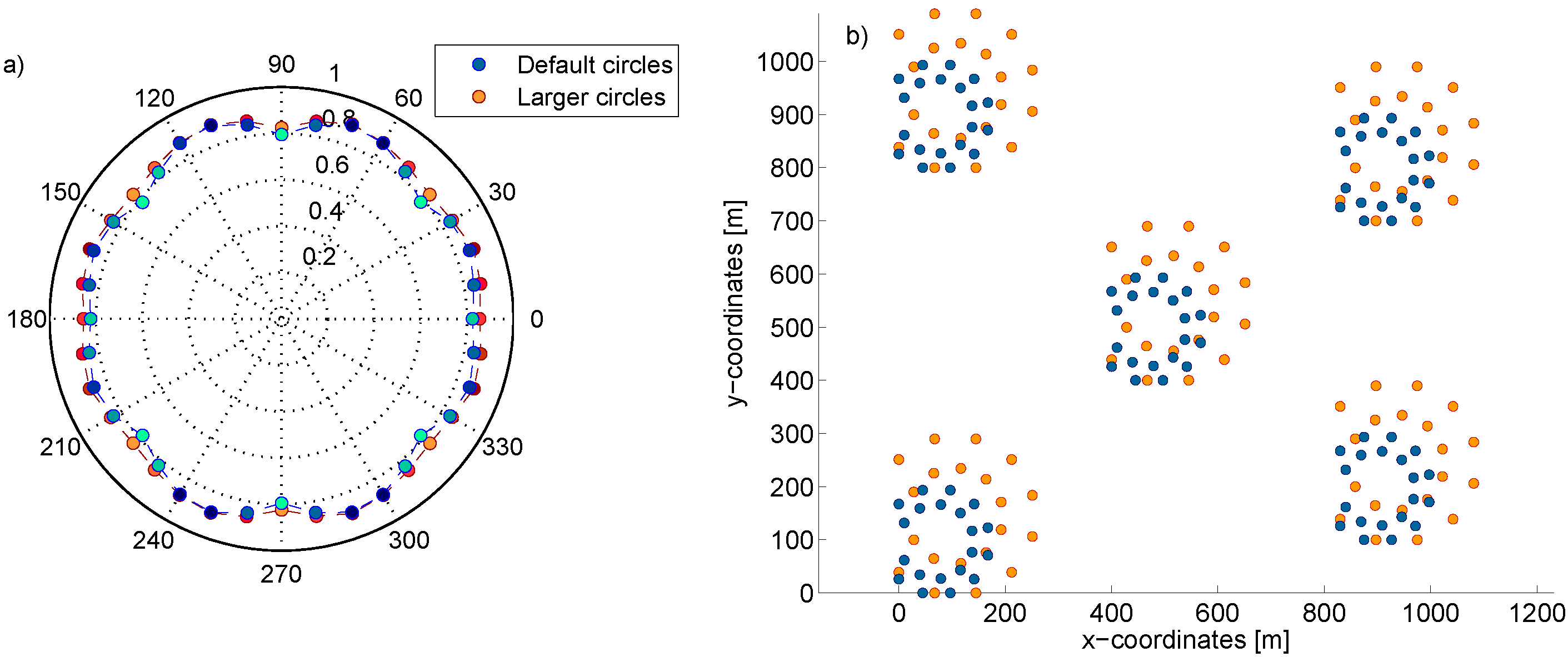
Figure 2. (a) Interaction factor q (radial coordinate in the plot) of an array with 100 WECs (shown in Figure 2b), as a function of incident wave angle. An angle of zero degrees corresponds to the configuration in Figure 2b and Figure 3 with the incident wave along the x-axis. The blue/cyan points correspond to the default smaller circles, whereas the red/orange points correspond to the larger circle configuration. (b) Configuration of the two farms with 100 WECs in five double circles with different inner and outer radii.

Figure 2. (a) Interaction factor q (radial coordinate in the plot) of an array with 100 WECs (shown in Figure 2b), as a function of incident wave angle. An angle of zero degrees corresponds to the configuration in Figure 2b and Figure 3 with the incident wave along the x-axis. The blue/cyan points correspond to the default smaller circles, whereas the red/orange points correspond to the larger circle configuration. (b) Configuration of the two farms with 100 WECs in five double circles with different inner and outer radii.

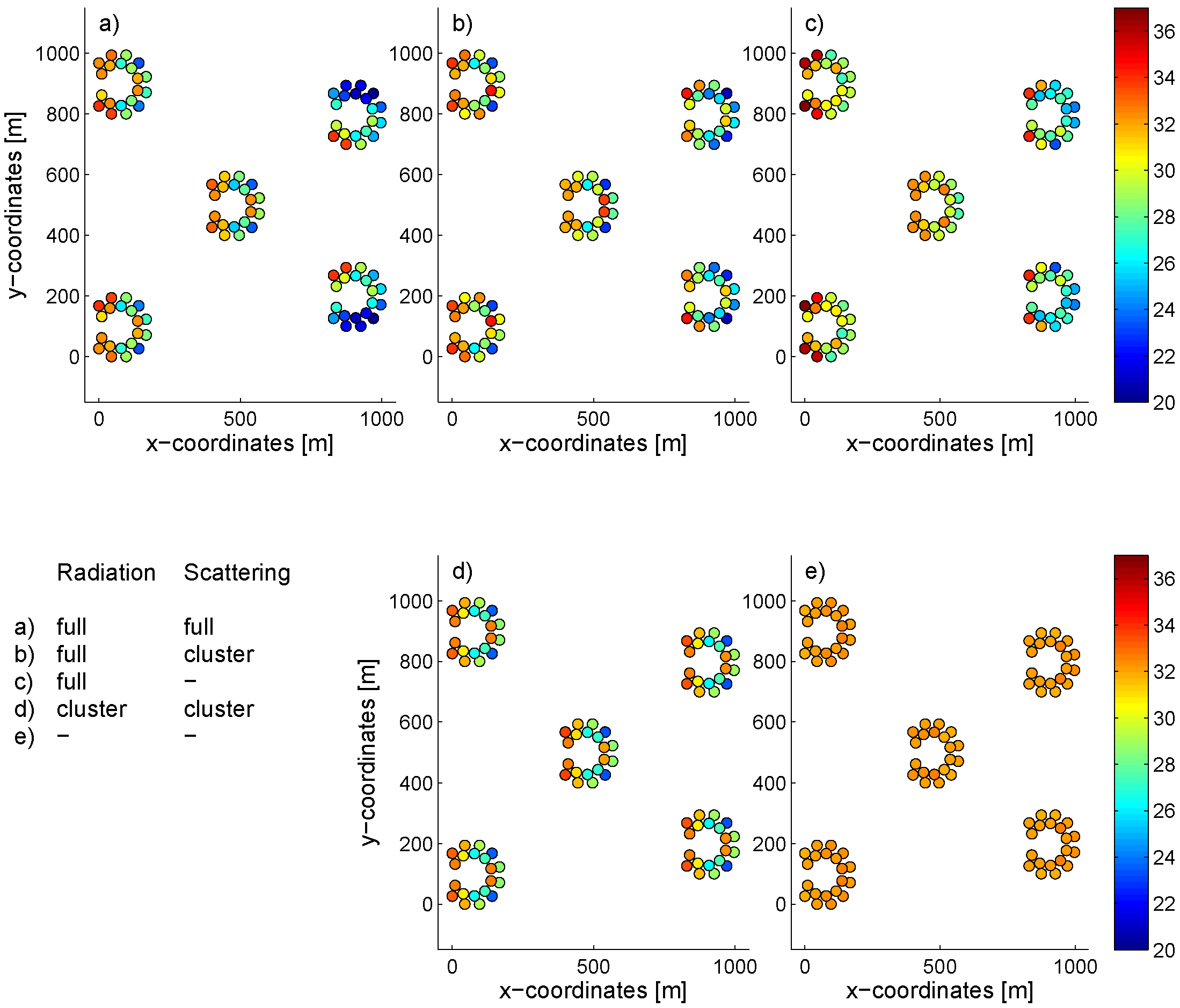
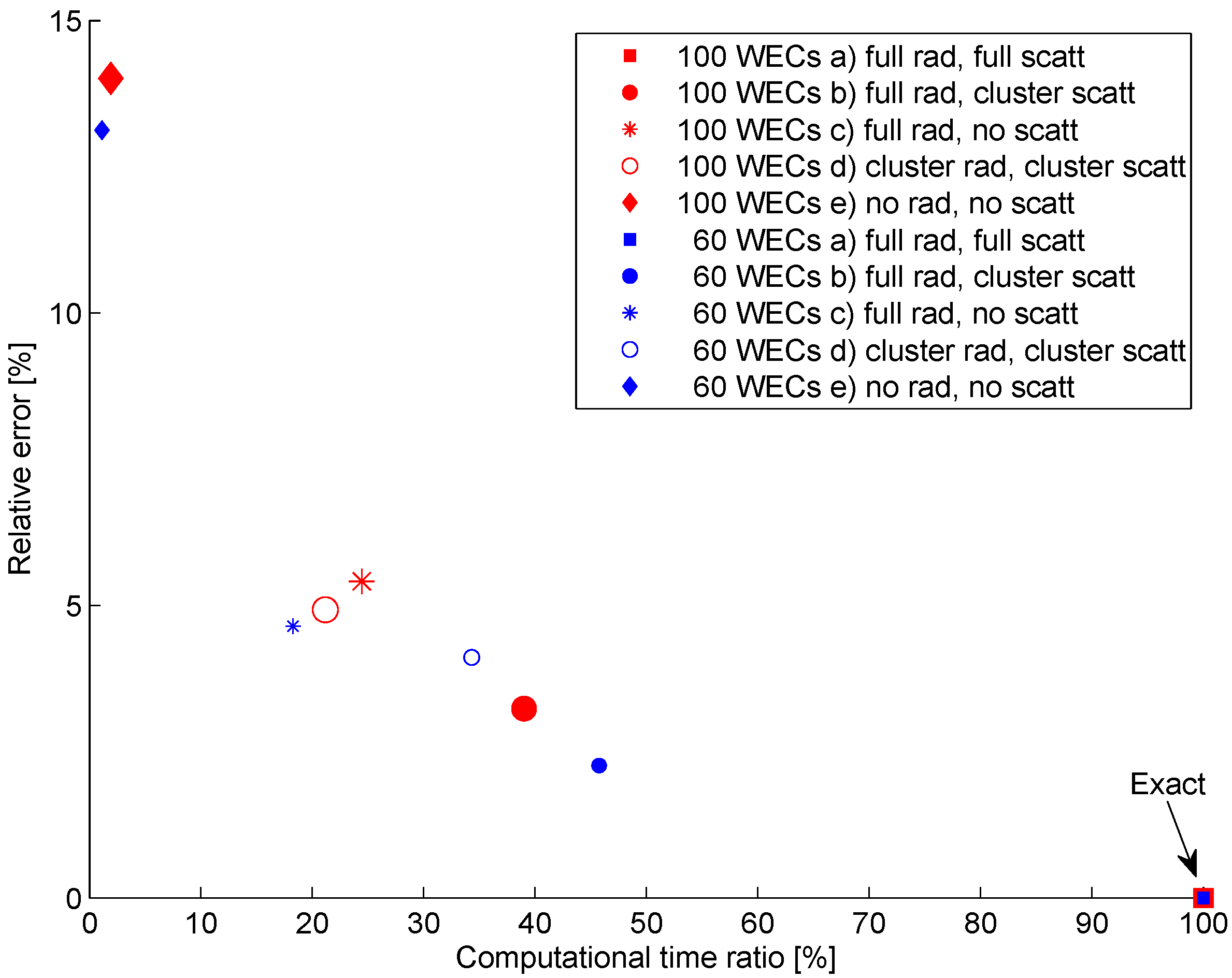
Figure 3. Farm of 100 WECs divided into five clusters. The capture width ratio in % for each WEC is shown with the color bar. The hydrodynamic interaction between the devices has been computed in five different ways with decreasing accuracy, shown in the table. (a) Full interaction is computed between all devices for diffracted and radiated waves; (b) Radiated waves between all WECs are taken into account, but diffraction is computed only within each cluster; (c) All WECs interact with radiated waves, but no multiple diffraction interaction is included; (d) Interaction is computed only within the cluster, both for radiated and diffracted waves; (e) No hydrodynamic interaction between the devices.

Figure 3. Farm of 100 WECs divided into five clusters. The capture width ratio in % for each WEC is shown with the color bar. The hydrodynamic interaction between the devices has been computed in five different ways with decreasing accuracy, shown in the table. (a) Full interaction is computed between all devices for diffracted and radiated waves; (b) Radiated waves between all WECs are taken into account, but diffraction is computed only within each cluster; (c) All WECs interact with radiated waves, but no multiple diffraction interaction is included; (d) Interaction is computed only within the cluster, both for radiated and diffracted waves; (e) No hydrodynamic interaction between the devices.

The multiple scattering model presented in Section 2.1 with the integrated interaction distance cut-off presented in Section 2.3 has been implemented as a MATLAB code and connected to a time domain model with the time series of measured waves as the input. The system of equations in Equation (10) has been truncated at ${\Lambda }_z=20$ and ${\Lambda }_{\theta }=3$. The inversion of the diffraction matrix is computed using the object-oriented factorization algorithm of [29].

The computations of small arrays of nine WECs have been executed on a standard desktop PC with four parallel Intel${}^{\circledR }$ Xeon${}^{\circledR }$ 3.07-GHz processors and 6 MB RAM. The simulations with the software WAMIT have been performed on the same computer. The computations for large farms have been executed on eight parallel Opteron 6220 cores running at 3 GHz with 4 GB RAM each on the high performance computer cluster UPPMAX.

3. Results

To evaluate the method of interaction distance cut-off in multiple scattering, in Section 3.1, we compare the results with the software WAMIT. After ensuring the reliability of the exact analytical multiple scattering method, the effect of introducing an interaction distance cut-off is further analyzed. The method is used to study farm configurations of arrays with over 100 WECs in Section 3.2.

3.1. Accuracy and Efficiency of the Method

WAMIT is a fast and reliable state-of-the-art boundary element method based on potential flow theory that is used in industry and academia all over the world. In the paper, the simulations with WAMIT have been computed with the higher-order method for the body geometry and solution, and first order linear potential theory has been used. The panel method is used to solve for the velocity potential and fluid pressure on the submerged surfaces of the bodies, and the output is given in terms of the hydrodynamic forces. WAMIT may serve as a benchmark tool for wave energy arrays of small or intermediate size and is used for the validation of the analytical method presented in the paper. For very large farms, however, the software becomes too computationally demanding, even on a high performance computer cluster.

The analytical method is validated against the numerical software in Figure 4. The accuracy of different values of the interaction distance cut-off is also studied. The array is a configuration of nine WECs on a square lattice with increasing separating distances D between adjacent devices; see Figure 4c.

In Figure 4a, the average power per device is plotted as a function of the separating distance. The agreement between the analytical method with full interaction distance cut-off and the numerical values is excellent, which is also confirmed by Figure 4b, showing the real part of the excitation force for the WEC at $x=0$, $y=0$ m in an array with separation distance $D=10$ m.

The least accuracy is obtained if the array is computed with no hydrodynamical interaction between devices. As expected, the simulation gives a constant power output for all devices and separation distances, and the excitation force in Figure 4b displays no diffraction patterns. In between the extrema of no interaction and full interaction, any interaction distance cut-off can be chosen: a smaller interaction distance cut-off will speed up the simulations considerably, but also reduce the accuracy. In the figure, the simulations for the nearest neighbor (NN) interaction is shown, i.e., hydrodynamic interactions are included only for the WECs that are closest to each other. The simulations give a better agreement than the simulations with no interaction, as expected. An even better approximation is achieved with the next-to-nearest neighbor (NNN) interaction, i.e., the WECs in the outer corners interact only with the three closest WECs, whereas the WEC in the middle interacts with all other WECs. In the simulation shown in Figure 4a, the NN approximation gives an average relative error of 2.9% from the WAMIT value, whereas the NNN approximation would give an average relative error of 2.1%.

Figure 4. Accuracy of the analytical model, as compared to WAMIT. Simulations with the analytical model performed with no interaction, nearest neighbor (NN) interaction and full interaction between devices. (a) Average power per device in an array with nine WECs, as a function of separation distance D between adjacent devices; (b) The real part of the excitation force with increasing interaction distance cut-off; (c) The configuration of the array.

Figure 4. Accuracy of the analytical model, as compared to WAMIT. Simulations with the analytical model performed with no interaction, nearest neighbor (NN) interaction and full interaction between devices. (a) Average power per device in an array with nine WECs, as a function of separation distance D between adjacent devices; (b) The real part of the excitation force with increasing interaction distance cut-off; (c) The configuration of the array.

Another option is to set the interaction distance cut-off to a constant number, for example 50 m. The results will then follow the exact results as long as all devices are within 50 m from each other, but will take the same approximate values as the simulations with no interactions when all WECs are separated by more than 50 m [19]. The accuracy and time savings with different interaction distance cut-offs is further analyzed in Figure 5.

A farm of 100 WECs divided into five clusters is shown in Figure 3. The capture width ratio (Equation (17)) in % is shown for each device with the color bar. The hydrodynamical interactions between the devices in the farm are computed with different interaction distance cut-offs, so that the interaction is either computed between all devices, or only between devices within the same cluster, or neglected. This can be done for both the radiated and the scattered waves.

In all of the farms (a–c) in the upper row, the hydrodynamical interactions by radiated waves (non-diagonal terms in the radiation force) are included between all devices. In Farm (a), full interaction is computed between all devices for scattered and radiated waves, and the total power of the farm is computed as 0.97 MW. This is the target value that we will be referring to as the exact value, since it is exact within the assumptions of linear potential flow theory (up to the truncation of infinite sums). In Farm (b), multiple scattering effects are restricted to interact only within each cluster, and the total power is computed to be 1.00 MW. The multiple diffraction effects are neglected (point-absorber approximation) in Farm (c), giving a computed total power of 1.03 MW, i.e., an overprediction by 5%. In Farm (d), the interactions by both radiated and diffracted waves are computed only within the clusters (total power 1.02 MW), and in the last Farm (e), the hydrodynamical interactions are fully neglected (total power 1.11 MW).

Figure 5. Computational time ratio vs. relative error of farm simulations with the different interaction distance cut-off shown in Figure 3. The exact values (highlighted in the figure) are for farms with full diffraction and radiation interaction. The farms with 100 WECs are plotted in red, larger markers; the farms with 60 WECs in blue, smaller markers.

Figure 5. Computational time ratio vs. relative error of farm simulations with the different interaction distance cut-off shown in Figure 3. The exact values (highlighted in the figure) are for farms with full diffraction and radiation interaction. The farms with 100 WECs are plotted in red, larger markers; the farms with 60 WECs in blue, smaller markers.

To quantify the accuracy and the time savings of the interaction distance cut-off, the results of using different values of the interaction distance cut-off have been plotted in Figure 5. As benchmark values, the exact results from computing full interactions in the scattering and radiation problems are used, i.e., Farm (a)). The remaining simulations are plotted as ratios:

$$\begin{array}{c}\mathrm{Computational}\mathrm{time}\mathrm{ratio}=\frac{\mathrm{computation}\mathrm{time}}{{\mathrm{computation}\mathrm{time}}_{\mathrm{exact}}},\hfill \\ \mathrm{Relative}\mathrm{error}=\frac{\mathrm{total}\mathrm{absorbed}\mathrm{power}}{{\mathrm{total}\mathrm{absorbed}\mathrm{power}}_{\mathrm{exact}}}-1\hfill \end{array}$$

(20)

The results for farms with 100 WECs are plotted in red, larger markers. Equivalent results for a farm with 60 WECs, corresponding to the three clusters with the lowest y-coordinates in the farm with 100 WECs, are plotted in blue, smaller markers. For the benchmark, exact values are plotted as squares. Here, we see that ignoring all hydrodynamic interaction effects between devices (filled diamonds) will save more than 98% of the computational time, but have an error of around 13%–14%. Instead, neglecting the interaction between devices in different clusters (empty circles) will give a result that is around 5% off the exact value, to 20%–35% of the computational cost. Including full interaction for radiated waves, but neglecting all multiple scattering effects (asterisks) gives around the same error, but slightly more time savings. The best approximation is given by including full interaction for radiated waves, but scattering only within the clusters, which gives an error of 2%–3%, to around 40%–45% of the computational cost of the benchmark values. The simulations for 60 and 100 WECs follow the similar trend, but one can observe that the inter-cluster interactions are relatively more important for larger farms than for the smaller ones.

It is important to note that all of the approximative simulations overestimate the absorbed power for the farm.

3.2. Performance of Large Wave Energy Farms

The farms studied in this section are all computed with full interaction distance cut-off, i.e., multiple scattering that is exact up to the truncation of infinite sums.

The interaction factor q, sometimes referred to as the q-factor or interference effect factor, is often used to compare different array layouts. It is defined as the ratio between the absorbed power of the full farm and the power that would have been absorbed by the same number of isolated WECs,

$$q=\frac{P_{\mathrm{tot}}}{N\times P_{\mathrm{isolated}}}$$

(21)

A constructive interaction factor $q>1$ means that the WECs interact constructively, so that the total power absorbed by the farm is higher than it would have been if the devices were isolated. For large farms and in realistic, irregular sea states, a destructive interaction factor $q<1$ is more likely to occur. Since the performance of the farm depends on the incident wave direction, it is important to investigate the interaction factor as a function of wave propagation angles and to avoid array configurations that have large destructive interactions.

The interaction factor of the array in Figure 3, with 100 WECs in five clusters, has been plotted as a function of different incident wave angles in Figure 2a (blue markers). As can be seen in the figure, the farm configuration is rather insensitive to the incident wave direction; the interaction factor varies between 0.79 and 0.89, with the highest farm effect around incident wave angles of $\pm 20,70,110,160$ degrees and lowest for $\pm 40,90,140$. Since the interaction between devices in a farm is expected to decrease with increased distance between the devices [8,9], also a second farm configuration with 100 WECs in five larger circles has been studied. The two farm configurations are plotted in Figure 2b. The interaction factor of the farm with larger circles is plotted as a function of incident wave angle with red/orange markers in Figure 2a. The interaction factor of the farm with larger circle is slightly higher, $q\in [0.83,0.90]$, but the general trend for the two farms is the same: rather insensitive to wave direction and the lowest interaction factor for the same incident wave angles as the smaller circle.

Although the farm with larger circles has a larger interaction factor, one of its drawbacks is that the length of the sea cable will be increased, as compared to the layout with smaller circles. As the cost of sea cable is one of the major installation costs, this is an important point to consider. If all WECs in the farm are connected to an intermediate substation in the middle of each circle, the total cable length of a small circle is 1.68 km, compared to 2.37 km for a large circle.

To get a good estimate of the performance of a farm in realistic conditions, the farm with 100 WECs in Figure 3 has been studied for long time series of irregular waves measured at the off-shore test site in Lysekil, the west coast of Sweden, during the full month of January 2015. The result is plotted in Figure 6b and shows how the total performance of the farm depends on the significant wave height and energy period. The total absorbed power is shown in MW with the color bar and is computed as the time average of the instantaneous absorbed power of the full farm at each time instance. The average significant wave height and energy period for these 31 days were $H_s^{\mathrm{avg}}=1.58$ m, $T_e^{\mathrm{avg}}=6.4$ s, which gave an average total power absorption of $P_{\mathrm{total}}^{\mathrm{avg}}=1.35$ MW during the month.

One of the major reasons for deploying WECs in large arrays is to reduce the power fluctuations and deliver electricity of good quality to the grid. The ratio between the instantaneous power $P_{\mathrm{tot}}\left(t\right)$ and the time-averaged power of the farm with 100 WECs in Figure 3 is plotted during 20 min in Figure 6a and compared to the equivalent plot for a single device. It can be seen that the power peaks of the single device are sometimes over 12-times the average value, whereas the maximal power peaks for the farm are below three-times the average. The absorbed power for the single device and farm in this sea state is 12 kW and 973 kW, respectively, which shows the magnitude of the destructive interaction effects in the farm, since no interaction would imply a total power of $100\times 12$ kW.

Figure 6. (a) Ratio between instantaneous power $P_{\mathrm{tot}}\left(t\right)$ and time-averaged power of a single WEC (gray) and the farm of 100 WECs (black) with the configuration shown in Figure 3; (b) The total absorbed power (MW) for the same farm with 100 WECs, as a function of the energy period and significant wave height. All waves measured at the Lysekil test site during January 2015 have been used, separated into sea states of 30 min each.

Figure 6. (a) Ratio between instantaneous power $P_{\mathrm{tot}}\left(t\right)$ and time-averaged power of a single WEC (gray) and the farm of 100 WECs (black) with the configuration shown in Figure 3; (b) The total absorbed power (MW) for the same farm with 100 WECs, as a function of the energy period and significant wave height. All waves measured at the Lysekil test site during January 2015 have been used, separated into sea states of 30 min each.

4. Discussion

The physical interpretation of the interaction distance cut-off can be seen clearly in Figure 3. When no hydrodynamic interaction between devices is considered, as in Figure 3e, all WECs display the same power absorption. When interaction is considered only within the clusters, all clusters are equal, as can be seen in Figure 3d.

The computations (c) in Figure 3 and Figure 5 are performed for an infinite interaction distance cut-off for the radiated waves, but zero interaction distance cut-off for the diffracted waves. This is the same as the point-absorber approximation; the non-diagonal terms in the radiation force are included, but only single-body diffraction is computed. Hence, Figure 3, Figure 4 and Figure 5 shed light on the validity of the point-absorber approximation in comparison to the exact computations and also to other valid approximations. For a farm with 100 WECs in five clusters, we see that the point-absorber approximation is comparable in accuracy and time-savings with computations where multiple diffraction and interaction by radiated waves are included only for devices within the same cluster.

In [30], it was shown that the interaction factor integrated over all incident wave angles equals unity, implying that if there are destructive interaction factors for some incident wave angles, they must be positive for other angles. An underlying assumption for that computation is that the single devices perform at resonance, so that maximum power is absorbed. The resonance condition is not satisfied by the WECs studied in this paper; hence, a destructive interaction factor can be expected for all wave angles. One goal of the optimization of the farm configuration is then to minimize the destructive interactions to avoid the lowest interaction factor values. The interaction factor q for the farm in Figure 3 has been plotted as a function of incident wave angle in Figure 2 and shows that the farm configuration is rather insensitive to the incident wave angle.

The hydrodynamical interaction between devices decreases with increasing separation distance between the devices [8,9]. To study this effect, the interaction factor has been studied for the same farm configuration,, but with larger double circles; see Figure 2b. The interaction factor is increased slightly; hence, the destructive interaction effects are lower in the larger circles. On the other hand, if the WECs are all connected to a substation at the center of the circles, the cable length for connecting all of the WECs is increased for the configuration with larger circles. These two design parameters, lowering the destructive interaction factor and reducing cost for sea cable, must be weighed against each other, the preferred choice depending on the price per produced kW electricity versus the cost of cable.

5. Conclusions

An analytical model for the hydrodynamic interactions in wave energy farms has been developed based on the multiple scattering method. To reduce computational cost, but retain high accuracy, the interactions are included only between devices within an arbitrarily-specified interaction distance cut-off. With infinite interaction distance cut-off, the method is exact up to the truncation of infinite sums and within the assumptions of linear potential flow theory, and excellent agreement with state-of-the-art numerical software is achieved for the arrays where both methods can be applied. The interaction distance cut-off can be chosen differently for the interaction by radiated and diffracted waves, and the accuracy of different values of the interaction distance cut-off has been investigated. Whereas an approximation of no hydrodynamical interactions for a farm with 100 WECs gives a result for the total power output, which is 14% off the exact value (to less than 2% of the computational cost), a good approximation is achieved when full interaction by radiated waves is included, but multiple scattering is computed only for devices that are close. The relative error is then only 2%–3%, to less than 50% of the computational cost.

The method has been used to study the instantaneous power output and power fluctuations of wave energy farms with 60–120 WECs operating in irregular waves measured off-shore on the Swedish west coast. One month of continuous wave data has been used in the simulations, and the time-averaged power output for each 30-min sea state ranged up to 10 MW.