2.1. Wave Data
Adequate buoy data are not available off the coast of Brazil; thus, the dataset used for the present work is derived from the European Centre for Medium-Range Weather Forecasts (ECMWF) data set. The ECMWF is a meteorological data assimilation project, where an atmosphere circulation reanalysis is integrated with a wave model. Weather predictions are based on the implementation of weather observations collected over decades through a single consistent analysis in forecast models. Operatively, a meteorological future state is derived on how the climate systems evolve with time from an initial condition. The sea state is described by the two-dimensional wave spectrum. No wave parameters are assimilated, making the sea surface conditions a hindcast run, where forecasts have always relied on accurate observations of the current weather. The dataset used is termed ERA-Interim (ECMWF Reanalysis from 1979 onward), continuously updated in real time. Significant wave height (H
s), mean period (T
m) and mean direction (θ
m), ranging from January 2004, to December 2014, were extracted from the ERA-Interim archive, available for download online [
46]. This dataset constitutes the basis of the analyses conducted in this paper.
The Atlantic Ocean is covered by the base model grid with a resolution of 0.75° × 0.75°. In order to analyze the direct interaction between composited meteorological conditions of the wind field and ocean waves, very large temporal and spatial domain should be taken into account.
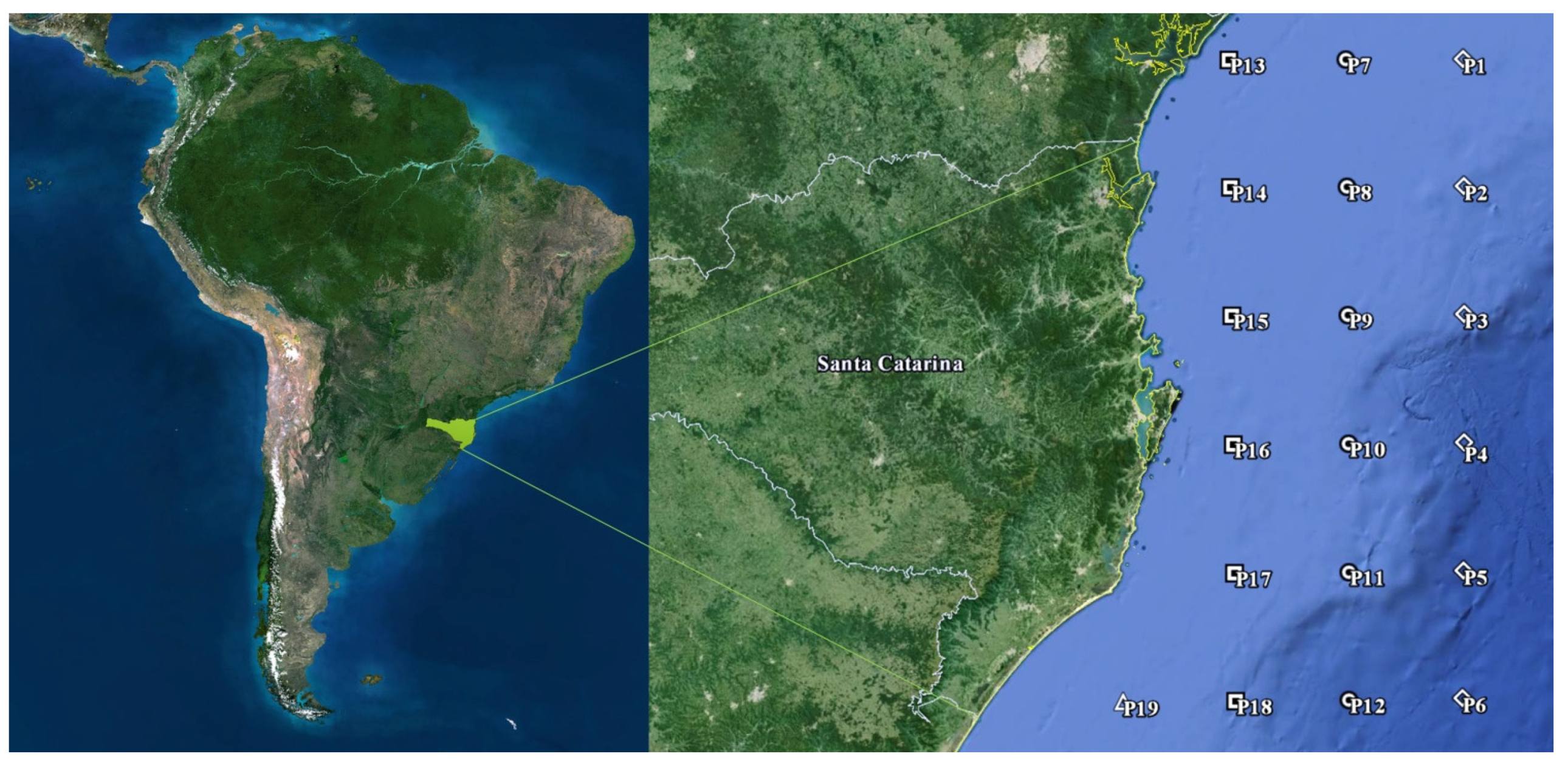
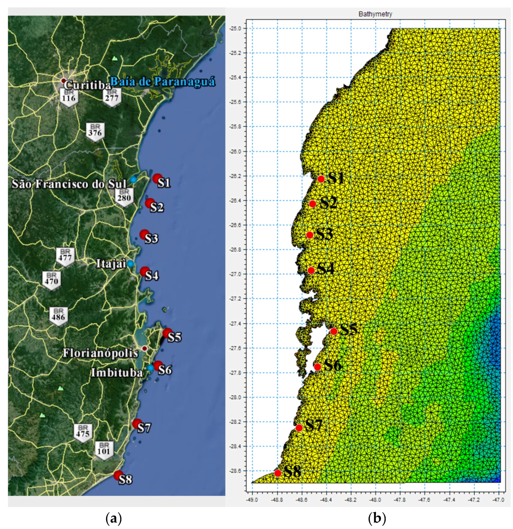
The approach to directly use the wave parameters instead of wind data, in further accordance with the dimension of coastlines, allows to analyze the variability of offshore wave power, but reducing the observational scale and, in turn, the number of reference points from ECMWF. Therefore, 19 grid points (P1–P19) were considered necessary, and have been selected to cover a latitude from 25.5°S to 29.25°S with a longitude ranging from 46.5°O to 48.75°O (
Figure 1).
The geographical coordinates of the offshore points, and their distance from the coastline and seabed, are shown in
Table 1.
Table 1.
Geographical information of European Centre for Medium-Range Weather Forecasts (ECMWF) grid points P1–P19.
Table 1.
Geographical information of European Centre for Medium-Range Weather Forecasts (ECMWF) grid points P1–P19.
| Point | Distance from Coast (km) | Depth (m) | Lat | Lon |
|---|
| P1 | 133 | 104 | 25°30′0.00′′S | 46°30′0.00′′O |
| P2 | 188 | 236 | 26°15′0.00′′ S | 46°30′0.00′′ O |
| P3 | 210 | 445 | 27°0′0.00′′S | 46°30′0.00′′O |
| P4 | 187 | 1646 | 27°45′0.00′′S | 46°30′0.00′′O |
| P5 | 214 | 2024 | 28°30′0.00′′S | 46°30′0.00′′O |
| P6 | 235 | 2306 | 29°15′0.00′′S | 46°30′0.00′′O |
| P7 | 76 | 55 | 25°30′0.00′′S | 47°15′0.00′′O |
| P8 | 126 | 101 | 26°15′0.00′′S | 47°15′0.00′′O |
| P9 | 118 | 144 | 27°0′0.00′′S | 47°15′0.00′′O |
| P10 | 114 | 270 | 27°45′0.00′′S | 47°15′0.00′′O |
| P11 | 136 | 301 | 28°30′0.00′′S | 47°15′0.00′′O |
| P12 | 165 | 1553 | 29°15′0.00′′S | 47°15′0.00′′O |
| P13 | 21 | 20 | 25°30′0.00′′S | 47°0′0.00′′O |
| P14 | 44 | 54 | 26°15′0.00′′S | 48°0′0.00′′O |
| P15 | 49 | 65 | 27°0′0.00′′S | 48°0′0.00′′O |
| P16 | 45 | 91 | 27°45′0.00′′S | 48°0′0.00′′O |
| P17 | 72 | 125 | 28°30′0.00′′S | 48°0′0.00′′O |
| P18 | 110 | 277 | 29°15′0.00′′S | 48°0′0.00′′O |
| P19 | 64 | 91 | 29°15′0.00′′S | 48°45′0.00′′O |
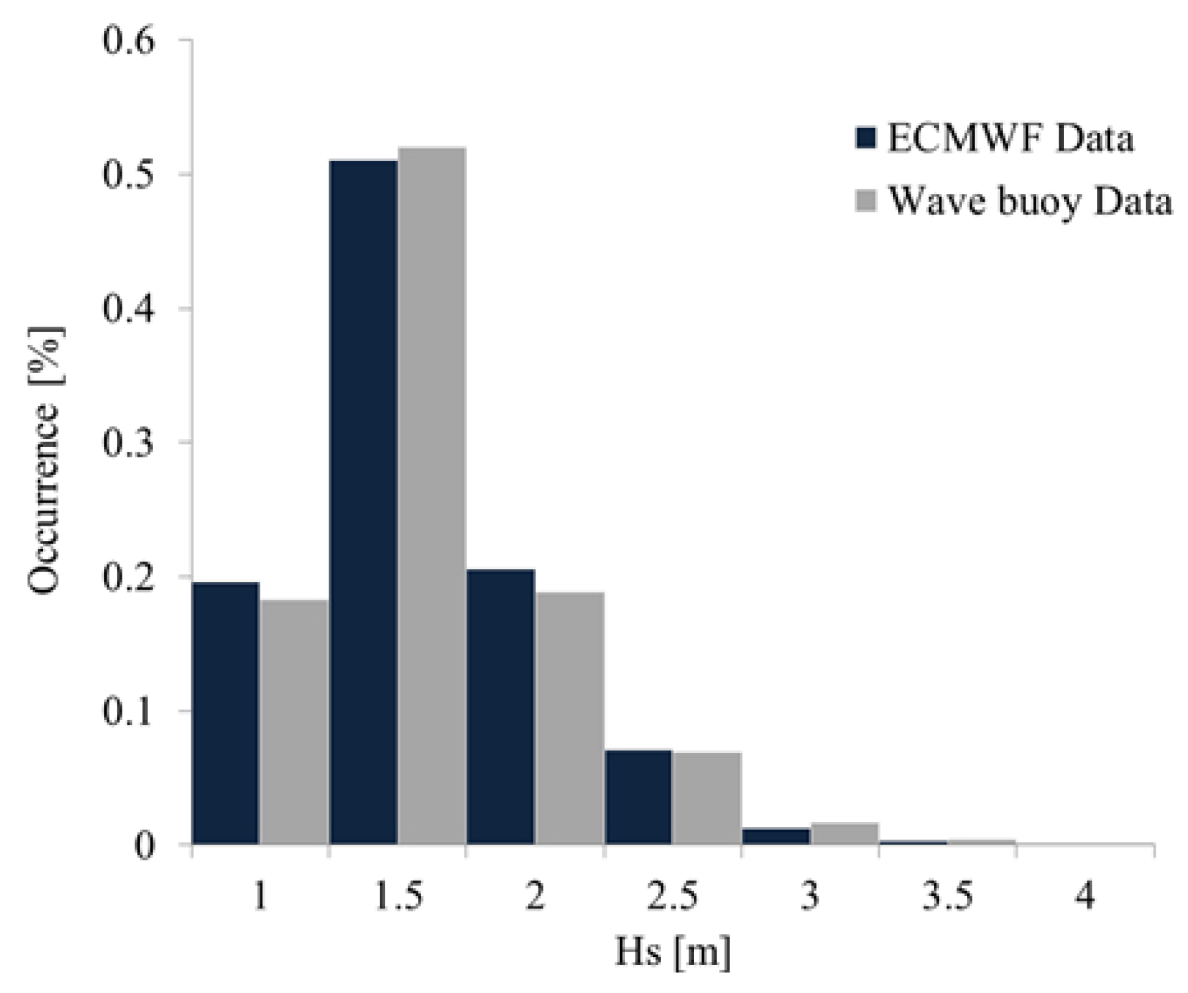
The ECMWF model uses the currently best description of the model physics, thus, the hindcasts from it can be considered reliable. Detailed data validation is not possible since only limited, measured wave time series are available for the region of interest [
47].
2.2. Method
The offshore wave climate at any arbitrary site is comprised of a superposition of wave fields, including swells propagating from several distant sources and “sea” waves generated by local winds.
The energy flux or power,
P, transmitted by a regular wave per unit crest width can be written as a vertical section of unit width, perpendicular to the wave propagation direction, equal to:
in which
Cg is the group velocity. For natural a sea state, where waves are random in height, and period (and direction), the spectral parameters have to be used. The wave energy flux can be defined as:
where
ρ is the sea water density,
g is the gravity acceleration,
f is the frequency,
h is the water depth,
S(f,θ) denotes the directional spectral density function, and
Cg(f,h) denotes the wave group velocity, expressed as:
where
k is the wave number.
Wave height computation is based on zero-order moment of the spectral function, and is readily estimated as follows:
In the method, the energy period,
Te, is the preferred period parameter. The reason can be found in the conceptual definition of energy period; as the period of the sinusoidal wave that has the same parametric height and the same power density of the considered sea-state. In deep water, it can be defined in terms of the minus-one and the zeroth spectral moments:
where
mn represents the spectral moment of order
n.
The offshore wave power is not affected by refraction and shoaling, and can be computed directly from hindcast wave data using the approximate deep water expression (
i.e., where h > L/2), simplified to:
From each hindcast point, the 6-h pair dataset was obtained. For each pair, the related power series was calculated. Furthermore, the power series was analyzed in order to get monthly and yearly power. Operatively, from the 6-h triple (
Hs,
Tm,
θm) provided by the ERA-interim for grid points P1–P19, a 10-year averaged 6-h triple dataset was obtained. Then, the corresponding energy period,
Te, was computed. The energy period is rarely specified and must be estimated from other variables (e.g., mean or peak period) when the spectral shape is unknown. When the peak period
Tp is known, a possible approach could be assumed.
where the coefficient
α depends on the frequency spectrum model.
The coefficient
α was assumed equal to 1 in the assessing of the wave energy resource in Southern New England [
48]. General speaking,
α increases towards unity with decreasing spectral width [
49]. In fact, for a Pierson-Moskowitz spectrum, which is only used for fully developed seas [
50],
α = 0.86 could be assumed, whereas for a standard JONSWAP (JOint North Sea WAve Project) spectrum with a peak enhancement factor of
γ = 3.3,
α reaches 0.90. The Santa Catarina real sea state is comprised of multiple wave systems,
i.e., a local wind sea plus more swells approaching from different directions. It is beyond the scope of this study to evaluate correspondence of the spectral distributions to the spectrum model. Furthermore, being unknown, the peak period, a relationship with the mean period, should be used. In preparing the Atlas of UK Marine Renewable Energy Resources [
51], it was assumed that
Te = 1.14
Tm. This approach seems more conservative, despite a direct correlation with peak period in the study area, where very long-period swell can be recognized. Therefore, it has been adopted in this study. Finally, the related power series was calculated using Equation (1). The power series were analyzed in order to get monthly and yearly power.
2.3. Results
The main parameters of wave climate at each grid point are reported in
Table 2. The overall wave climate is characterized by overall averaged wave parameters, with a significant wave height of 1.76 m, a mean period of 8.07 s, and a mean direction of 126°. Very low variability around these mean values has been found, as confirmed by the small standard deviation of significant wave height and mean period for each point and averaged over the whole dataset (respectively
σH,
σT and
σ in
Table 2).
Table 2.
Main wave climate parameters (based on 10-year average) at ECMWF grid points.
Table 2.
Main wave climate parameters (based on 10-year average) at ECMWF grid points.
| Point | Hs,mean | Hs,max | Hs,min | σH | Tm, mean | Tm, max | σT | Te,mean | θm |
|---|
| (m) | (m) | (m) | (m) | (s) | (s) | (s) | (s) | (°) |
|---|
| P1 | 1.64 | 4.14 | 0.75 | 0.49 | 8.23 | 14.27 | 1.25 | 9.39 | 132 |
| P2 | 1.76 | 4.59 | 0.77 | 0.54 | 8.27 | 14.50 | 1.29 | 9.43 | 130 |
| P3 | 1.85 | 4.94 | 0.78 | 0.58 | 8.25 | 14.47 | 1.33 | 9.40 | 129 |
| P4 | 1.94 | 5.34 | 0.80 | 0.61 | 8.24 | 14.30 | 1.35 | 9.39 | 128 |
| P5 | 2.02 | 5.62 | 0.82 | 0.64 | 8.22 | 13.98 | 1.36 | 9.37 | 127 |
| P6 | 2.09 | 5.82 | 0.84 | 0.67 | 8.20 | 14.00 | 1.37 | 9.35 | 128 |
| P7 | 1.41 | 3.68 | 0.66 | 0.41 | 7.94 | 13.92 | 1.17 | 9.06 | 129 |
| P8 | 1.57 | 4.19 | 0.71 | 0.47 | 8.04 | 13.85 | 1.22 | 9.16 | 127 |
| P9 | 1.68 | 4.49 | 0.73 | 0.51 | 8.06 | 14.14 | 1.28 | 9.19 | 126 |
| P10 | 1.82 | 5.04 | 0.77 | 0.56 | 8.12 | 14.13 | 1.33 | 9.25 | 125 |
| P11 | 1.94 | 5.44 | 0.79 | 0.60 | 8.12 | 13.91 | 1.35 | 9.26 | 125 |
| P12 | 2.04 | 5.68 | 0.81 | 0.65 | 8.11 | 14.16 | 1.36 | 9.25 | 125 |
| P13 | 1.38 | 3.79 | 0.65 | 0.41 | 7.81 | 13.88 | 1.17 | 8.91 | 124 |
| P14 | 1.38 | 3.79 | 0.65 | 0.41 | 7.81 | 13.88 | 1.17 | 8.91 | 124 |
| P15 | 1.36 | 3.76 | 0.62 | 0.39 | 7.70 | 13.77 | 1.20 | 8.78 | 124 |
| P16 | 1.83 | 5.17 | 0.76 | 0.56 | 8.10 | 14.18 | 1.36 | 9.23 | 124 |
| P17 | 1.96 | 5.53 | 0.76 | 0.61 | 8.04 | 14.28 | 1.37 | 9.16 | 123 |
| P18 | 1.95 | 5.51 | 0.76 | 0.61 | 8.03 | 14.42 | 1.35 | 9.16 | 123 |
| P19 | 1.74 | 4.98 | 0.68 | 0.54 | 7.99 | 14.70 | 1.32 | 9.11 | 124 |
| Mean | 1.76 | 4.82 | 0.74 | 0.54 | 8.07 | 14.14 | 1.29 | 9.20 | 126 |
| σ | 0.24 | 0.74 | 0.06 | 0.09 | 0.16 | 0.26 | 0.07 | 0.18 | 2.66 |
Table 3 summarizes the seasonal and yearly mean power at each point. Standard deviation of power,
σP, and the yearly energy flux in MWh/m are also reported. The seasonal data are regrouped according to the following months: January, February, and March (Summer); April, May, and June (Autumn); July, August, and September (Winter); and October, November, and December (Spring). The annual wave power was found to range between about 9 kW/m (P13) and 21 KW/m (P6), with a gross mean of 15.2 kW/m and a standard deviation based on all data points,
σP, of 3.9 kW/m.
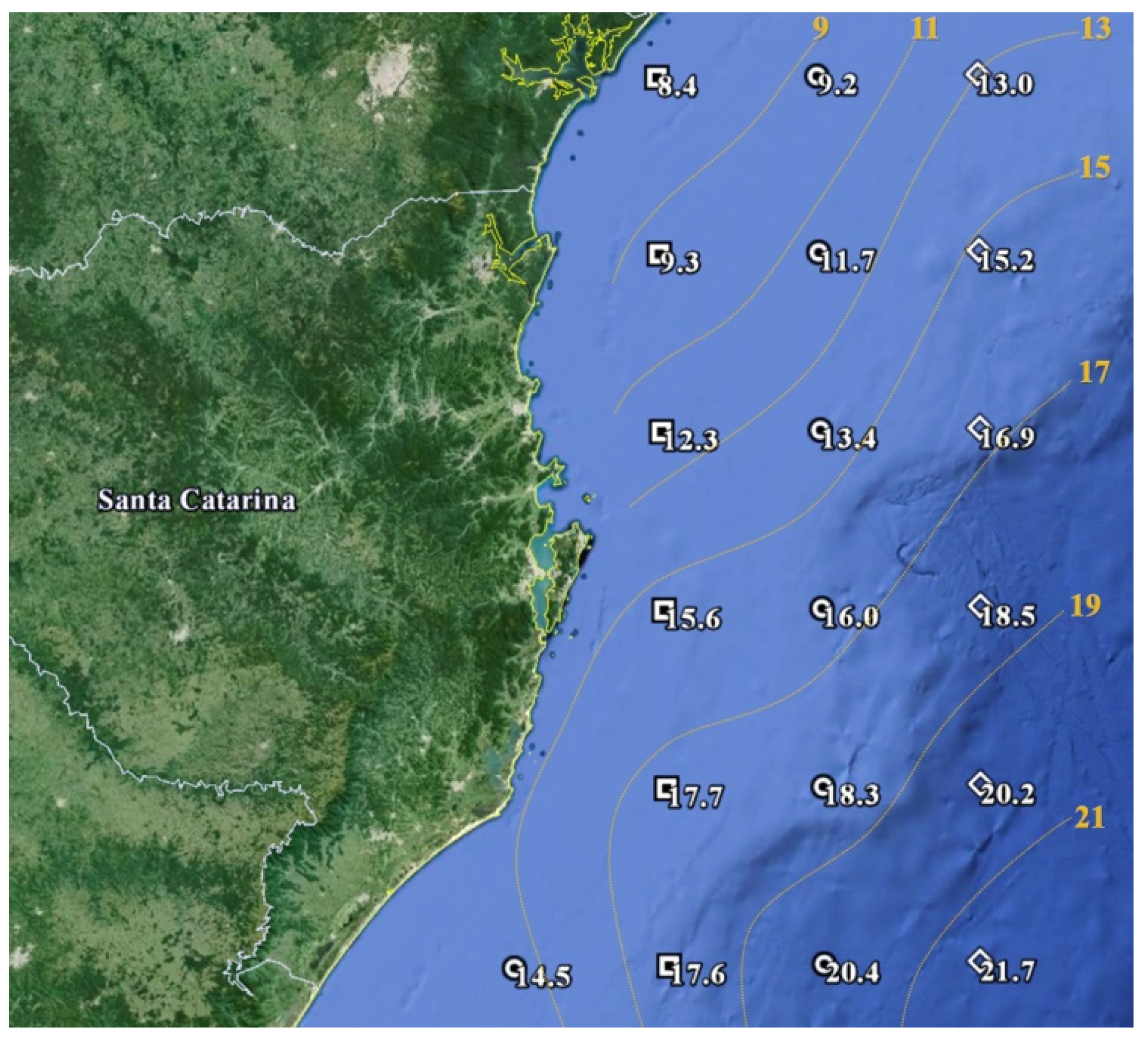
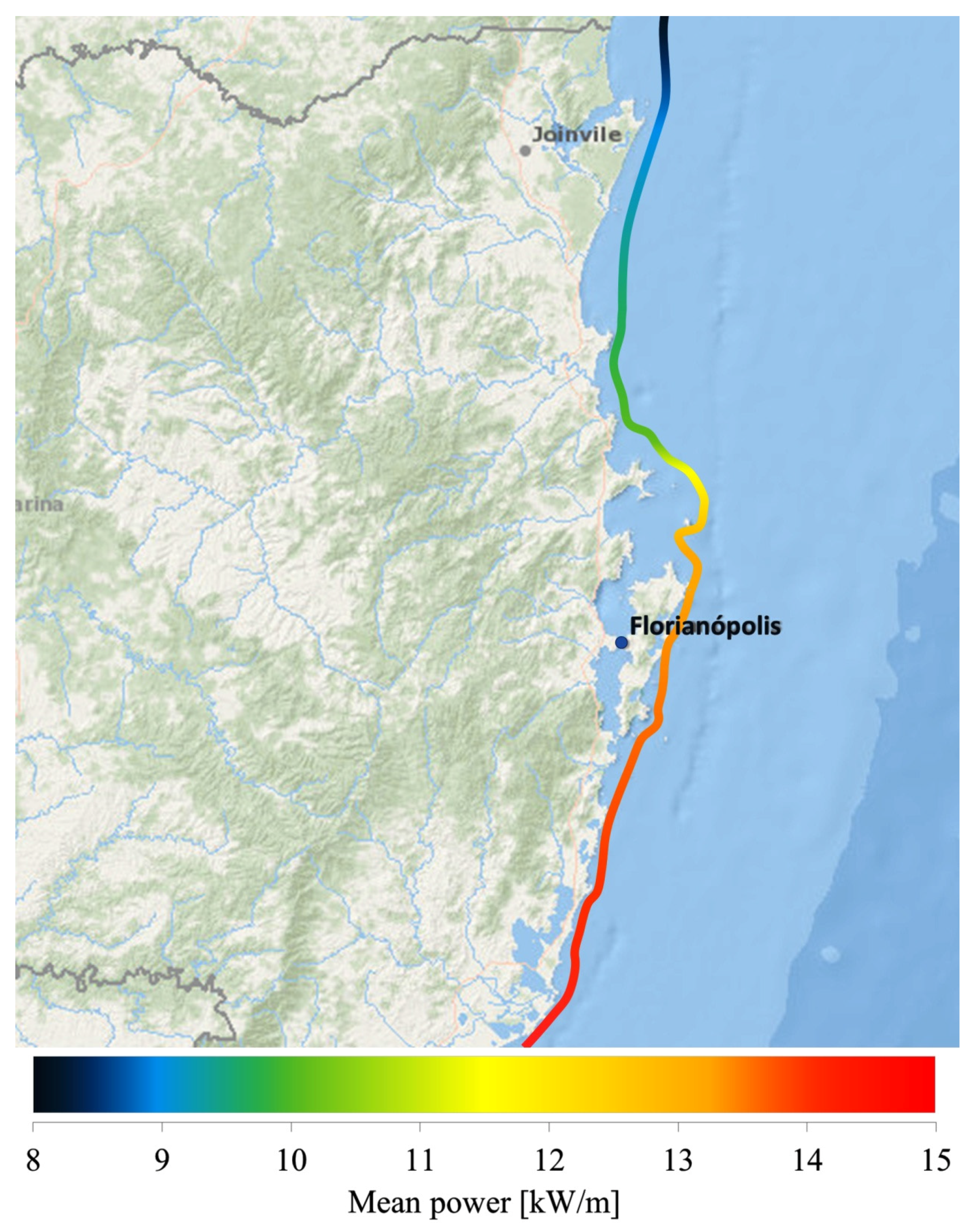
A tentative contour map (based on interpolation of power rate at 19 grid points) has been provided in
Figure 2, where wave power isolines, spacing 2 kW/m, are depicted, ranging from 8 to 22 kW/m.
Considering only the grid point in deep water (
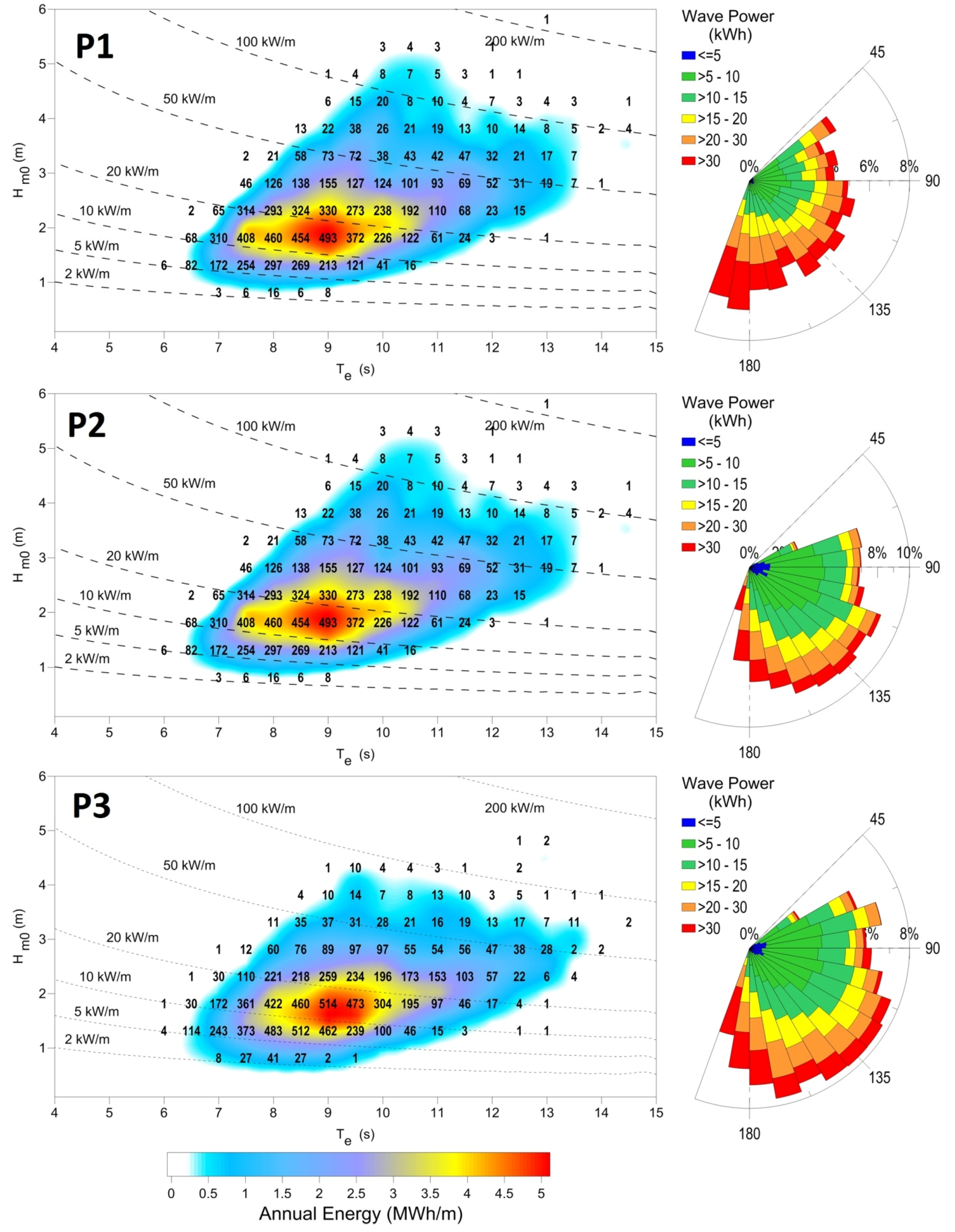
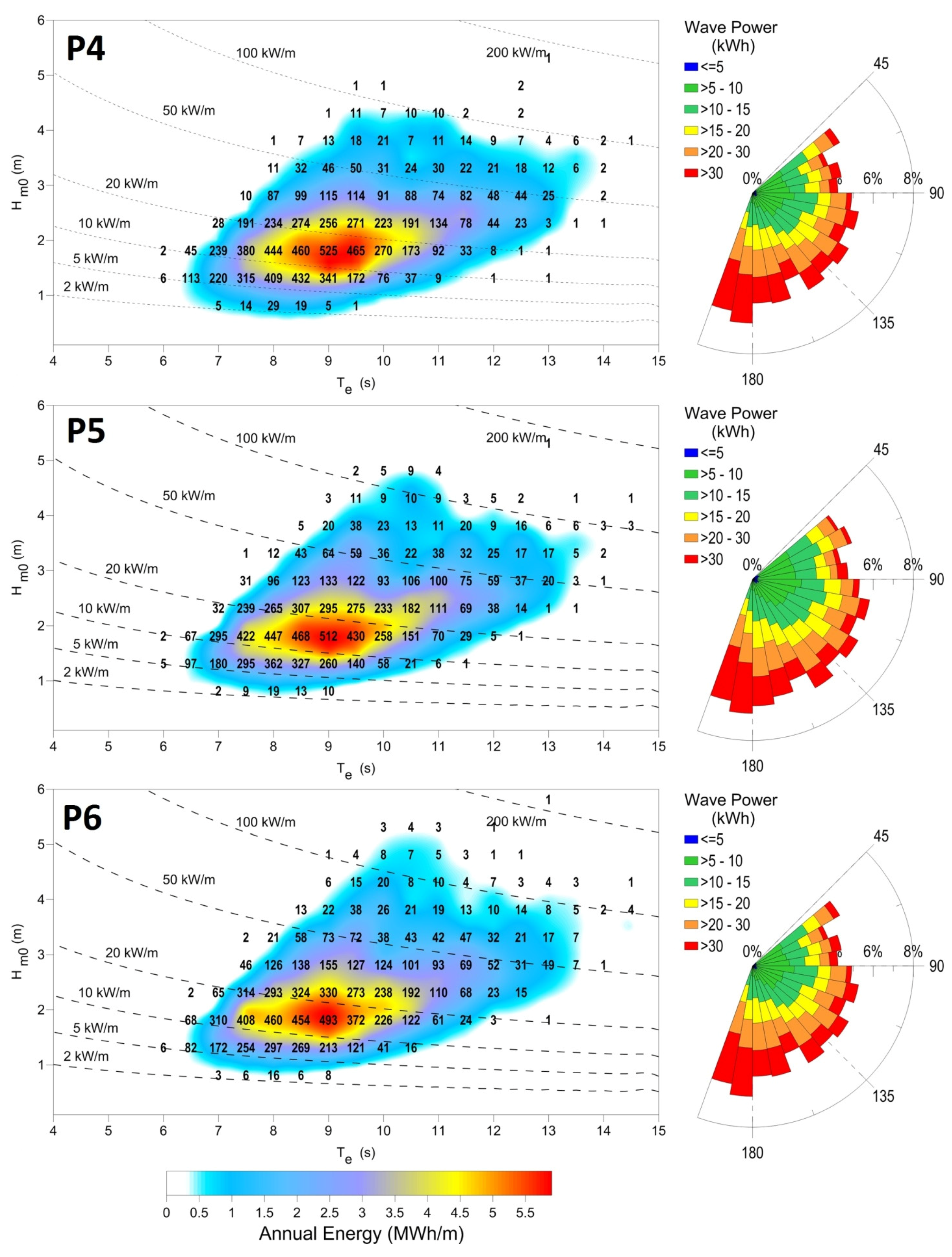
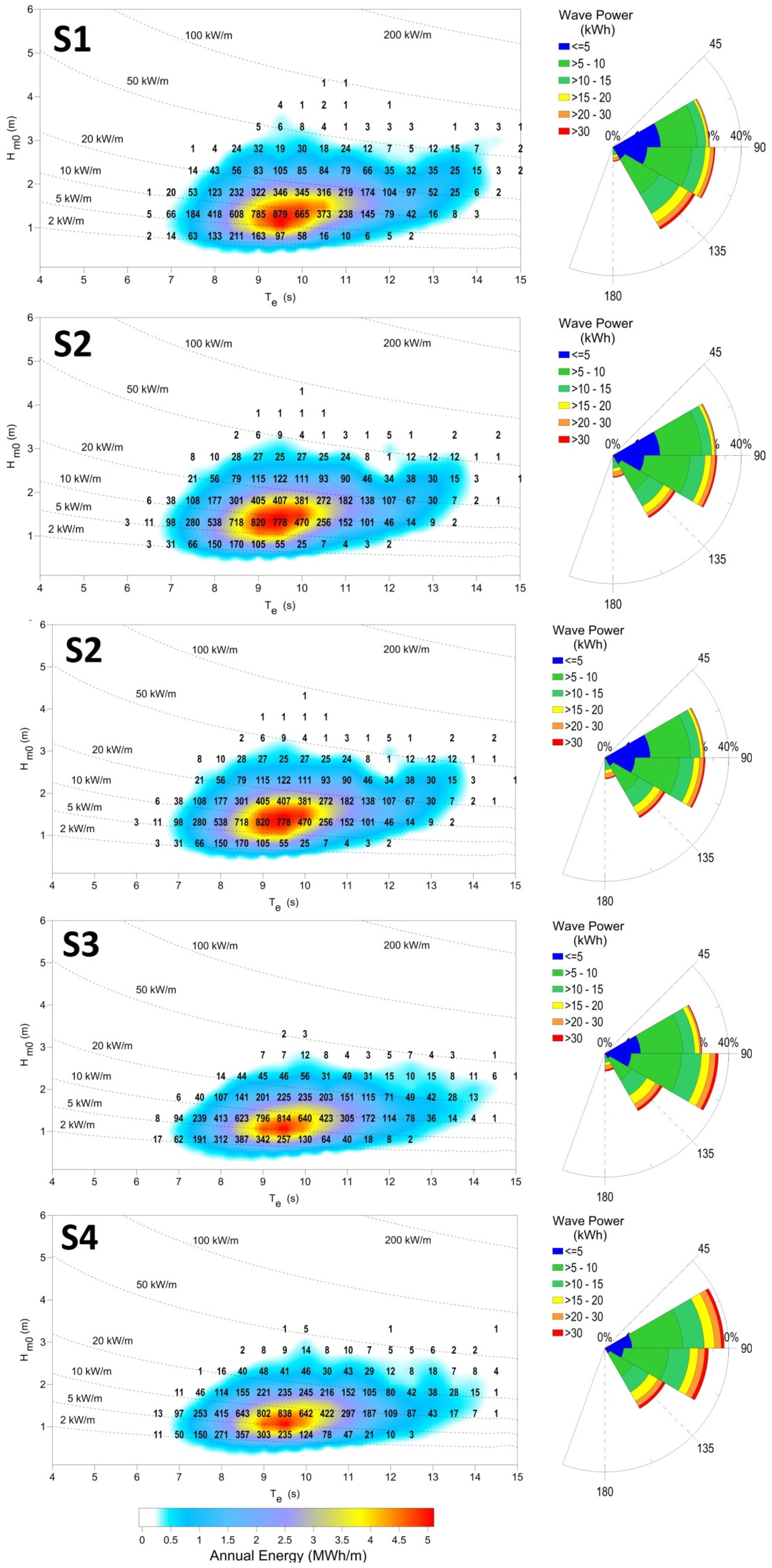
i.e., >70 m water deep), hence excluding points P7, P13 and P14, the energy density averaged on the whole offshore region is approximately equal to 16.4 kW/m. Focusing on the furthest from the shore grid points (on longitude 46.5°O), it is possible to note, in
Figure 3 and
Figure 4, that the bulk of the power is provided by south-southeast waves, with the south component being more dominant for increasing latitudes. The results are graphically represented by diagrams assembled in
Figure 3 and
Figure 4.
Table 3.
Average seasonal and yearly wave power (based on 10-year average) at ECMWF grid points.
Table 3.
Average seasonal and yearly wave power (based on 10-year average) at ECMWF grid points.
| Point | Average Yearly Power | Average Montly Power (kW/m) |
|---|
| (kW/m) | (MWh/m) | Spring | Summer | Autumn | Winter | σ |
|---|
| P1 | 13.00 | 113.87 | 11.58 | 10.09 | 14.89 | 15.42 | 2.58 |
| P2 | 15.18 | 132.98 | 13.41 | 11.72 | 17.48 | 18.12 | 3.11 |
| P3 | 16.86 | 147.67 | 14.72 | 12.99 | 19.56 | 20.16 | 3.55 |
| P4 | 18.52 | 162.19 | 15.90 | 14.08 | 21.77 | 22.31 | 4.14 |
| P5 | 20.15 | 176.48 | 17.08 | 15.11 | 23.87 | 24.53 | 4.75 |
| P6 | 21.73 | 190.35 | 18.24 | 16.08 | 25.82 | 26.77 | 5.36 |
| P7 | 9.21 | 80.71 | 8.53 | 7.40 | 10.23 | 10.71 | 1.53 |
| P8 | 11.65 | 102.05 | 10.62 | 9.29 | 13.04 | 13.65 | 2.04 |
| P9 | 13.43 | 117.68 | 12.05 | 10.62 | 15.21 | 15.85 | 2.51 |
| P10 | 16.01 | 140.26 | 14.02 | 12.40 | 18.52 | 19.10 | 3.31 |
| P11 | 18.29 | 160.19 | 15.73 | 13.88 | 21.42 | 22.12 | 4.10 |
| P12 | 20.37 | 178.47 | 17.30 | 15.18 | 23.98 | 25.03 | 4.87 |
| P13 | 8.38 | 73.42 | 7.95 | 6.94 | 9.06 | 9.57 | 1.17 |
| P14 | 9.32 | 81.68 | 8.85 | 7.72 | 10.08 | 10.65 | 1.30 |
| P15 | 12.31 | 107.87 | 11.69 | 10.22 | 13.30 | 14.04 | 1.71 |
| P16 | 15.57 | 136.41 | 13.64 | 12.06 | 18.03 | 18.56 | 3.22 |
| P17 | 17.74 | 155.42 | 15.30 | 13.40 | 20.70 | 21.57 | 4.01 |
| P18 | 17.59 | 154.07 | 15.22 | 13.30 | 20.43 | 21.40 | 3.94 |
| P19 | 14.47 | 126.78 | 12.84 | 11.26 | 16.56 | 17.23 | 2.88 |
| Mean | 15.25 | 133.61 | 13.40 | 11.78 | 17.58 | 18.25 | 3.16 |
| 3.92 | 34.32 | 3.01 | 2.69 | 4.94 | 5.05 | 1.25 |
Figure 2.
Ten-year averaged energy flux for the 19 ECMWF grid point and contour lines of the estimated mean wave power flux per unit crest on the Santa Catarina coastline.
Figure 2.
Ten-year averaged energy flux for the 19 ECMWF grid point and contour lines of the estimated mean wave power flux per unit crest on the Santa Catarina coastline.
Figure 3.
Characterization of the yearly average wave energy points P1, P2 and P3, in terms of significant wave height (Hm0) and energy period (Te). The color scale represents annual energy per meter of wave front (in MWh/m). The numbers within the graphs indicate the occurrence of sea states (in number of hours per year) and the isolines refer to wave power.
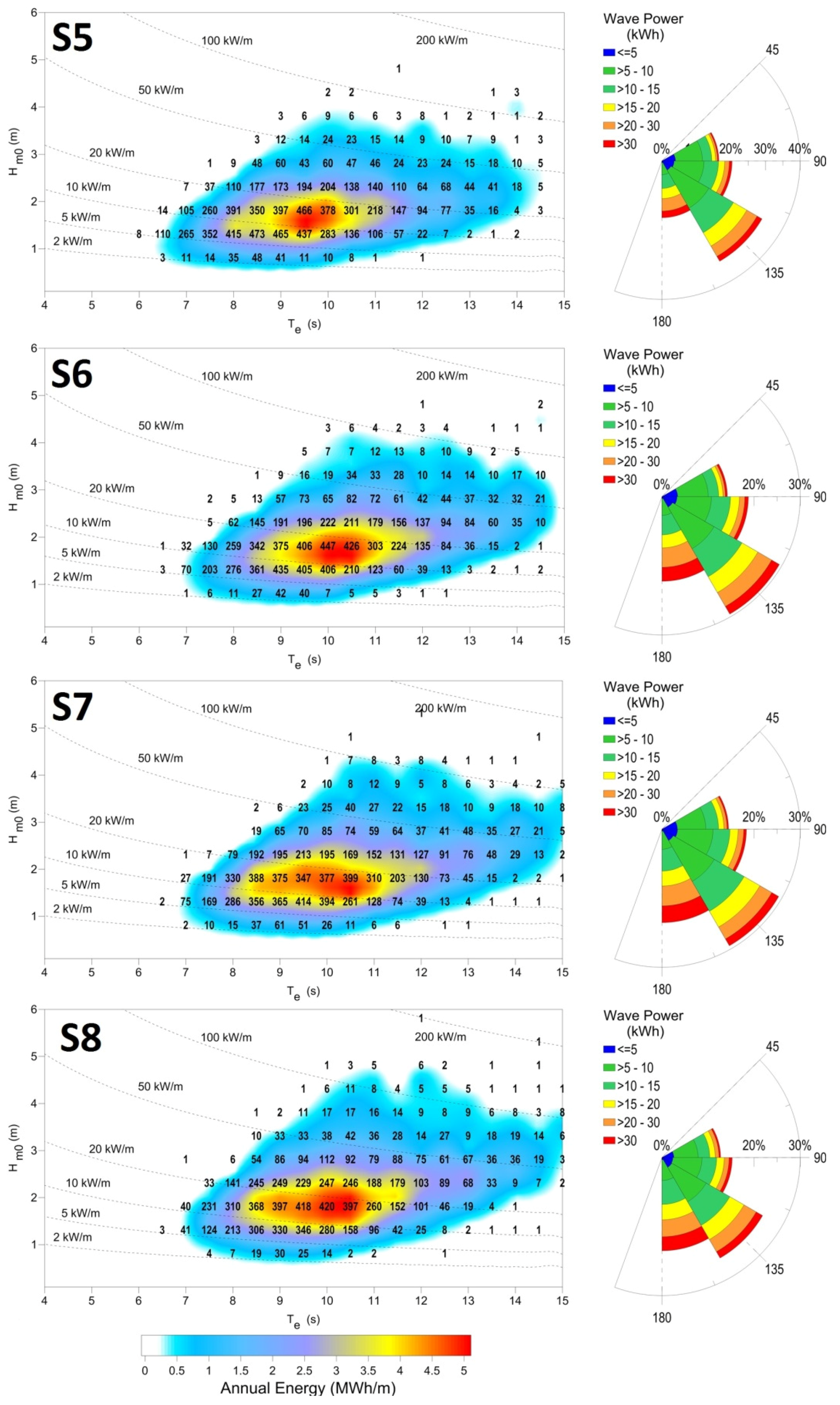
Figure 4.
Characterization of the yearly average wave energy points P4, P5, and P6 in terms of significant wave height (Hm0) and energy period (Te). The color scale represents annual energy per meter of wave front (in MWh/m). The numbers within the graphs indicate the occurrence of sea states (in number of hours per year) and the isolines refer to wave power.
About half of the annual wave energy (based on a 10-year average) is provided by waves with significant heights between 1.5 and 2.5 m and mean periods between 8 and 10 s (
Table 2).
Annual wave energy is distributed almost uniformly in all seasons. In particular, the mean percentages of power provided by each season are 22%, 19%, 29%, and 30% for Spring, Summer, Autumn and Winter, respectively.
The important seasonal stability registered in the area is due to weather factors of a large scale. Brazilian southern coast experiences a great regularity, regardless of seasonality [
52,
53,
54]. The principal reason is attributed to the rarity along South Atlantic Ocean of thunderstorms, organized on a large scale, such as hurricanes and tropical cyclones. This is the most remarkable feature of the South Atlantic weather system, completely opposite to its northern counterpart, which experiences hurricane season and, therefore, hurricane-generated waves. It is important to note, however, that South Atlantic tropical cyclones can be unusual weather events, but are not impossible. During March 2004, in fact, an extratropical cyclone formally transitioned into a tropical cyclone and made landfall on Brazil, after becoming a category 2 hurricane on the Saffir-Simpson hurricane wind scale. This storm, Cyclone Catarina, was defined as the first hurricane-intensity tropical cyclone ever recorded in the Southern Atlantic Ocean on 63 subtropical cyclones occurred between 1957 and 2007 [
55].
The major atmospheric perturbations in the study area are the cold fronts that cross the region. An average of six cold frontal systems per month, reaching South America, was defined [
56]. Monthly differences in wave power patterns can be related to the intensity and frequency of these meteorological systems, rather than their characteristics.
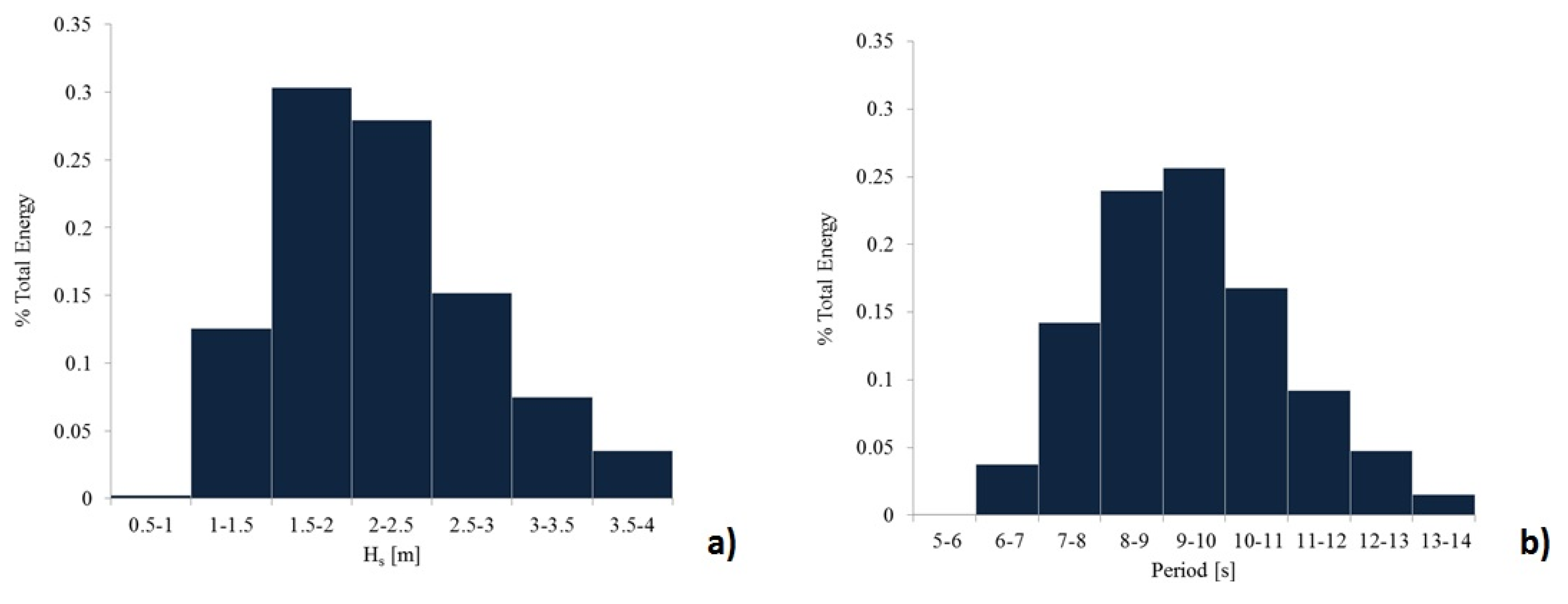
Wave characteristics reflect the wind regime over the South Atlantic, being the main share of energy flux supplied by south-southeast waves. Characterizing the wave energy source in terms of significant wave height at point P16, selected as more representative for the region of interest, it is highlighted in
Figure 5a as 58% of annual wave energy (based on a 10-year average), is provided by waves with significant heights of between 1.5 and 2.5 m. About 50% of the total annual resources are related to waves with peak periods between 8 and 10 s (
Figure 5b). For waves with periods greater than 10 s, the amount of energy is 32%, which is in accordance with the long fetch facing Santa Catarina and the above-mentioned local meteorological patterns.
Figure 5.
(a) Percentage of total wave energy vs. significant wave height at grid point P16; (b) Percentage of total wave energy vs. peak wave period at grid point P16.
Figure 5.
(a) Percentage of total wave energy vs. significant wave height at grid point P16; (b) Percentage of total wave energy vs. peak wave period at grid point P16.
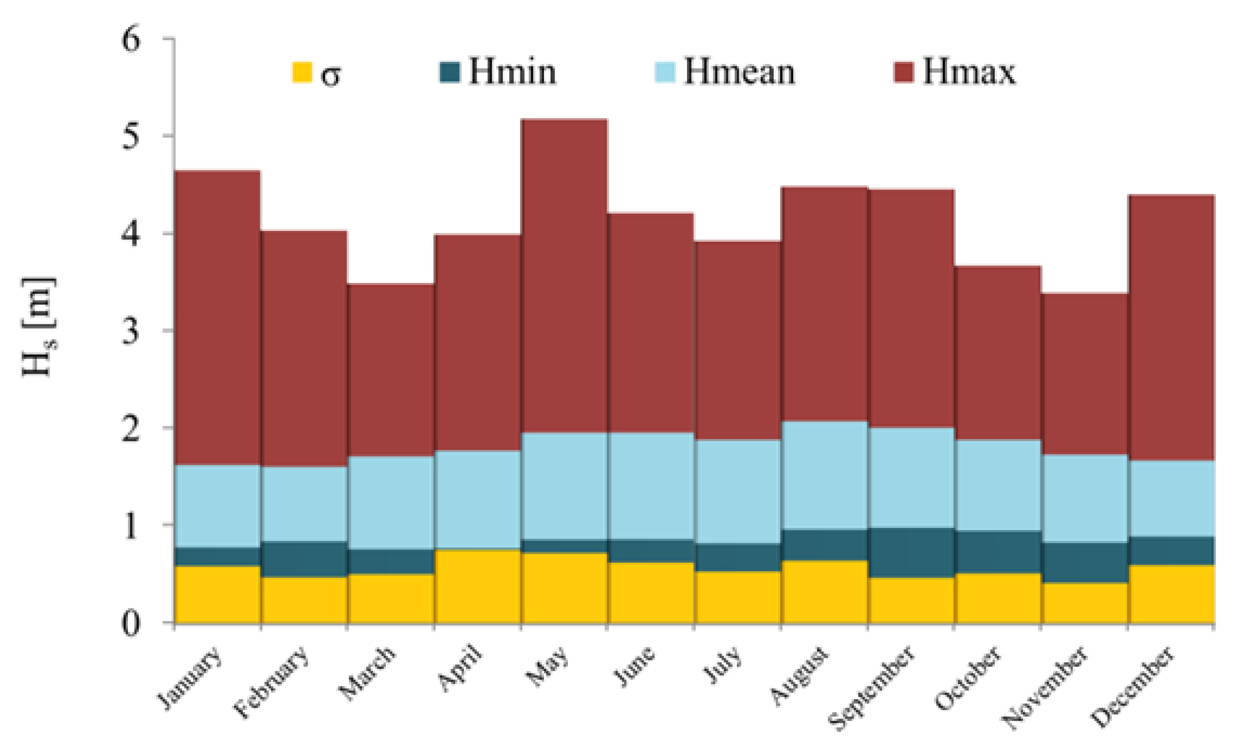
For the same point, P16,
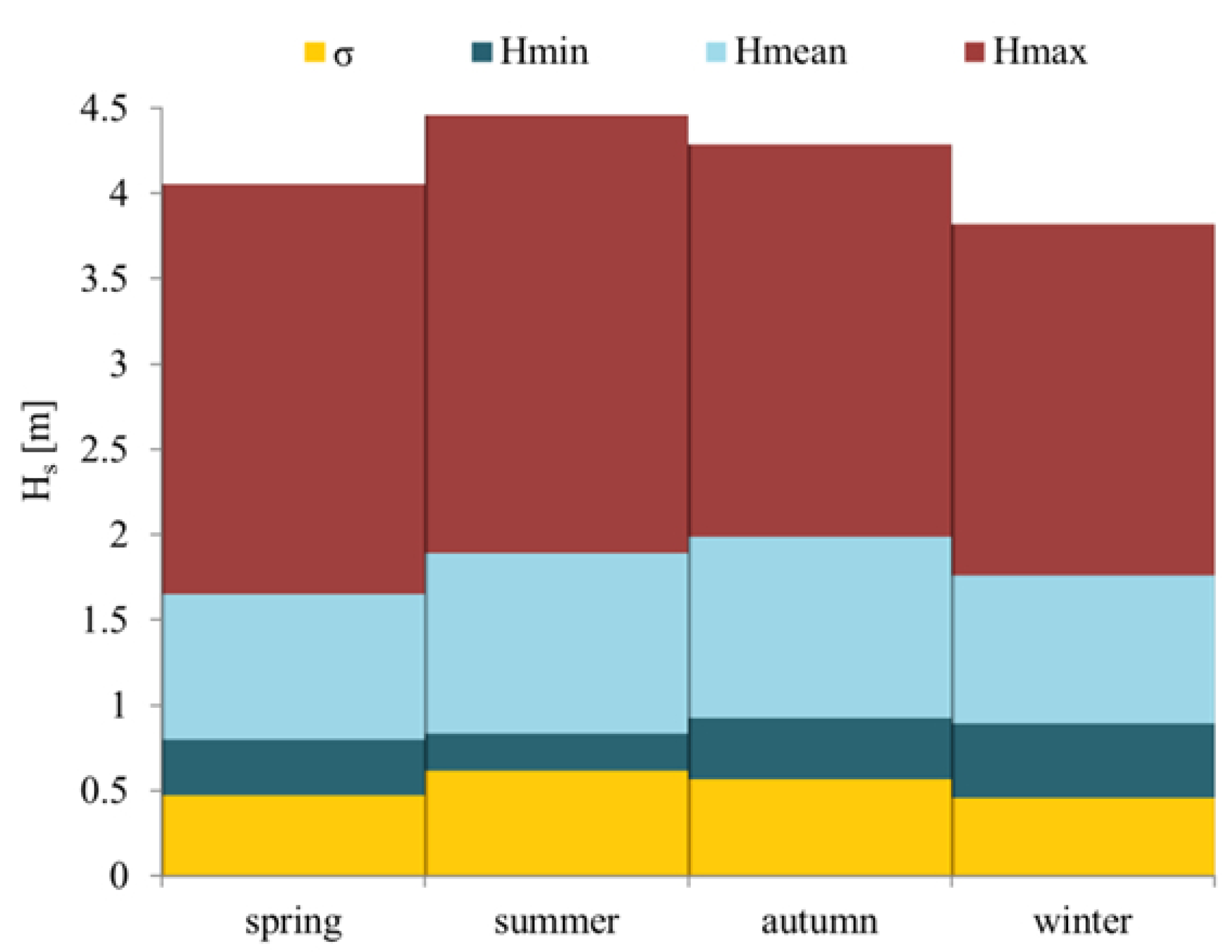
Figure 6 and
Figure 7 show, respectively, the monthly and seasonal distribution of the wave height patterns, averaged over the 10-year period of ECMWF wave forecasting data. The mean wave height is 1.83 m, ranging from 1.2 m and 1.7 m, respectively, in July and September. The maximum wave height was found to range between 3.8 m in January and 2.4 m in March, which is also the month where the minimum averaged wave height was found (0.65 m).
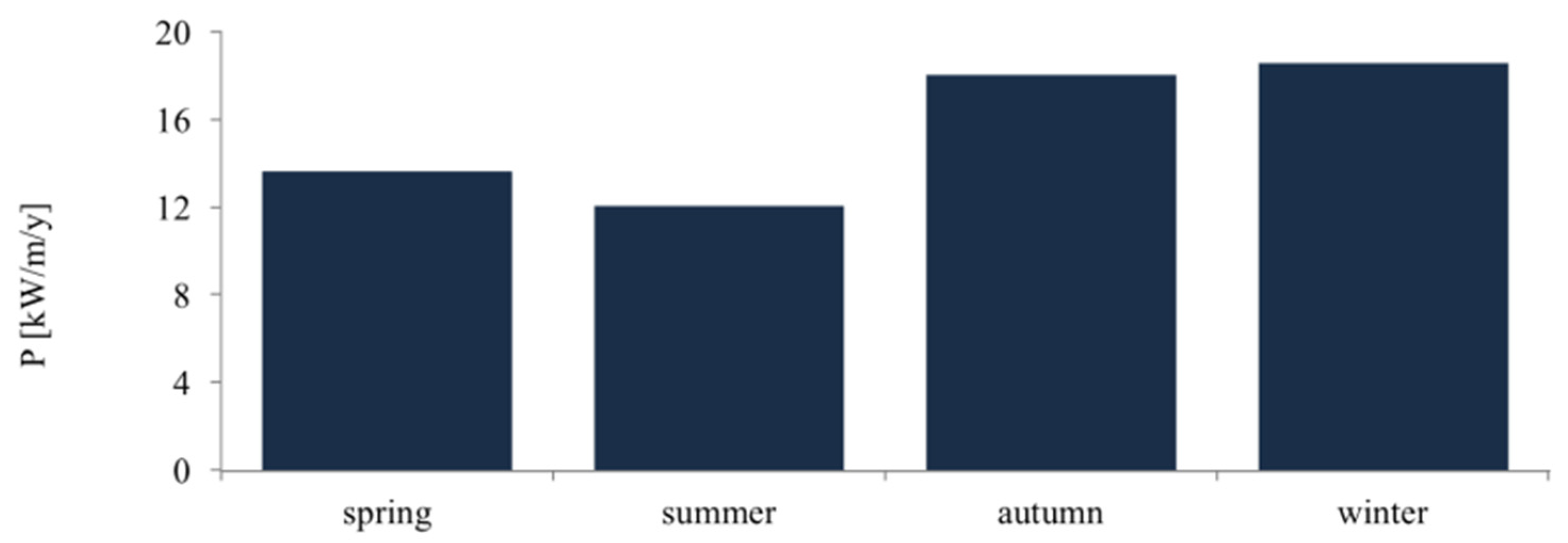
Whereas maximum averaged wave height is recorded in the summer period (from 21 December to 23 September), the energy flux in the winter period is higher than in the other periods (
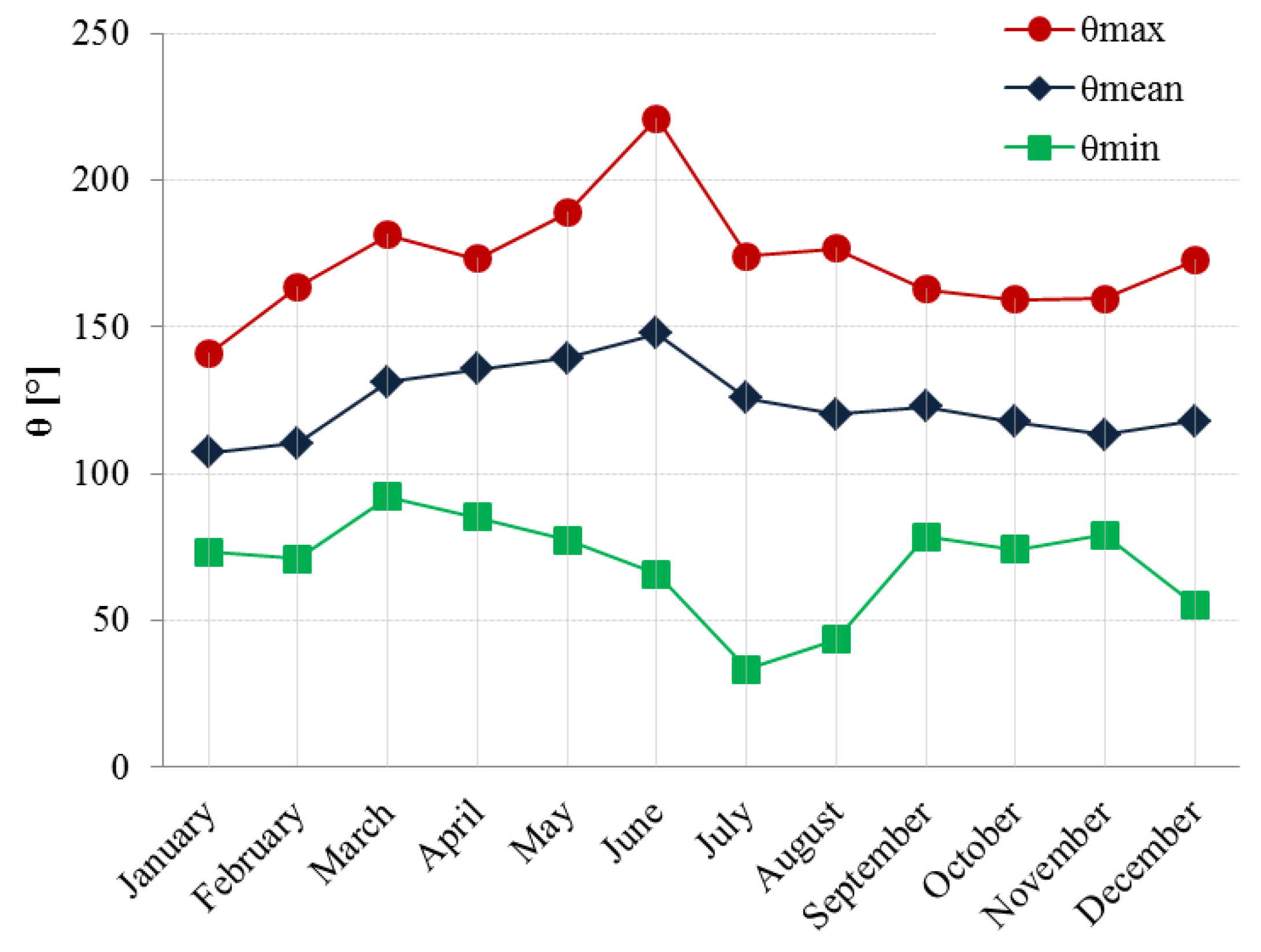
Figure 8), providing about 29.8% of total power. This value is not much higher than the autumn period (28.9%) and others seasons, which range approximately from 19.4% (Summer) to 21.9% (Spring). This poor seasonal dependence is also recognizable for wave direction, θ, shown in
Figure 9, a monthly stable wave energy flux sector. The dominant direction is 124°, with a monthly average ranging from 107° and 148°.
Figure 6.
Monthly wave climate characterization, in terms of significant wave height, averaged over 10 years at point P16.
Figure 6.
Monthly wave climate characterization, in terms of significant wave height, averaged over 10 years at point P16.
Figure 7.
Seasonal wave climate characterization, in terms of significant wave height, averaged over 10 years at point P16.
Figure 7.
Seasonal wave climate characterization, in terms of significant wave height, averaged over 10 years at point P16.
Figure 8.
Seasonal distribution of the wave energy flux, averaged over 10 years at point P16.
Figure 8.
Seasonal distribution of the wave energy flux, averaged over 10 years at point P16.
Figure 9.
Monthly distribution of the wave direction, averaged over 10 years at point P16.
Figure 9.
Monthly distribution of the wave direction, averaged over 10 years at point P16.


