1. Introduction
As the vertically integrated power industry evolves into a competitive market, electricity now can be treated as a commodity governed by demand and generation interactions. Competition among generating companies (GenCos) is highly encouraged in order to lower the energy price and benefit end consumers. However, when GenCos are given more flexibility to choose their bidding strategies, larger uncertainties are also brought into the electricity markets. Many factors that affect bidding strategies include the risk appetite of Gen Cos, price volatility of fuels, weather conditions, network congestion and overloading. These factors and their interactions may lead to larger price volatility in the deregulated power market.
Many efforts have been made to design and optimize the bidding strategies in the presence of uncertainty. Zhang
et al. [
1] proposed an efficient decision system based on a Lagrangian relaxation method to find the optimal bidding strategies of GenCos. Kian and Cruz [
2] modeled the oligopolistic electricity market as a non-linear dynamical system and used dynamic game theory to develop bidding strategies for market participants. Swider and Weber [
3] proposed a methodology that enables a strategically behaving bidder to maximize the revenue under price uncertainty. Centeno
et al. [
4] used a scenario tree to represent uncertain variables that may affect price formation, which include hydro inflows, power demand, and fuel prices. They also presented a model to analyze GenCos’ medium-term strategic analysis. In [
5], a dynamic bid model was used to simulate the bidding behaviors of the players and study the inter-relational effects of the players’ behaviors and the market conditions on the bidding strategies of players over time. Li and Shi [
6] proposed an agent-based model to study the strategic bidding in a day-ahead electricity market, and found that applying learning algorithms could help increase the net earnings of the market participants. Nojavan and Zare [
7] proposed an information gap decision theory model to solve the optimal bidding strategy problem by incorporating the uncertainty of market price. Their case study further shows that risk-averse or risk-taking decisions could affect the expected profit and the bidding curve in the day-ahead electricity market. Qiu
et al. [
8] discussed the impacts of model deviations on the design of a GenCo’s bidding strategies using the conjectural variation (CV) based methods, and further proposed a CV-based dynamic learning algorithm with data filtering to alleviate the influence of demand uncertainty. Kardakos
et al. [
9] point out that when making a bidding decision, a GenCo would take into accounts the behavior of its competitors as well as specific features and enacted rules of the electricity market. They further developed an optimal bidding strategy for a strategic generator in a transmission-constrained day-ahead electricity market. Other studies [
10,
11,
12] emphasized that transmission constraints, volatile loads, market power exertions, and collusions may induce GenCos to bid higher prices than their true marginal costs, thereby aggravating the price volatility issue.
As concern for the sustainability of the power market increases, efforts also have been made to reduce the risk of price variation. Most studies focus on the employment of price-based demand response (DR) programs for the electricity users to control and reduce the peak-to-average load ratio [
13,
14,
15,
16,
17,
18,
19,
20,
21,
22]. For instance, Oh and Hildreth [
13] proposed a novel decision model to determine whether or not to participate in the DR program, and further assessed the impact of the DR program on the market stability. Faria
et al. [
14] suggested that adequate tolls could motivate the potential market players to adopt the DR programs. Ghazvini
et al. [
15] showed that multi-objective decision-making is more realistic for retailers to optimize the resource schedule in a liberalized retail market. In [
16], a two-stage stochastic programming model was formulated to hedge the financial losses in the retail electricity market. Zhong
et al. [
17] proposed a new type of DR program to improve social welfare by offering coupon incentives. The researchers in [
18,
19] handled the energy scheduling issue by optimizing the DR program in a smart grid environment. Yousefi
et al. [
20] proposed a dynamic model to simulate a time-based DR program, and used Q-learning methods to optimize the decisions for the market stakeholders. In [
21,
22,
23], much more detailed reviews were provided for benefit analyses and applications of DR in a smart grid environment.
However, in electricity markets where the demand side is regulated, how to design and optimize GenCos’ bidding strategies is treated as one of the most efficient ways to sustain the market price in the presence of uncertainty. Some studies have been made by proposing an incentive mechanism or contract for the GenCos to mitigate the risk of price variation caused by their subjective preferences during the bidding process [
24,
25,
26,
27]. Silva
et al. [
24] introduce an incentive compatibility mechanism, which is individually rational and feasible, to resolve the asymmetric information problem. Liu
et al. [
25] proposed an incentive electricity generation mechanism to control GenCos’ market power and reduce the pollutant emissions using the signal transduction of game theory. Cai
et al. [
26] proposed a sealed dynamic price cap to prevent GenCos from exercising market power. Heine [
27] performed a series of studies on the effectiveness of regulatory schemes in energy markets, and pointed out that potential improvements exist in contemporary systems when incentive-based regulations are appropriately implemented.
Although there is a large body of literature in bidding and incentive policy, most of the studies neglect assessment of the long-term effects of the incentive programs on the GenCos’ learning behaviors. Besides, less attention is paid to the dynamic response of the GenCos to the volatile loads and incentive schemes. To maintain the market stability, it is highly desirable to understand the interplays between the incentive mechanism and the GenCos’ adaptive responses to the variable market. This paper aims to fill this gap by proposing an incentive mechanism in a day-ahead power market to reduce price variance, and further assessing the subsequent long-term impacts of the incentive mechanism. To that end, a two-level Stackelberg gaming model was developed to analyze the bidding strategies of the market participants including one independent system operator (ISO) and several GenCos. An optimal menu of incentive contracts was derived under a one-leader and multi-followers game theoretic framework. Finally, a Stackelberg-based Q-learning approach was employed to assess the GenCos’ response to the incentive-based generation mechanism.
The remainder of the paper is organized as follows: in
Section 2, we introduce the menu of incentive contracts, and describe the workflow of the multi-agent game framework; in
Section 3, we give a mathematical description of the problem, and present the details of the Stackelberg model; in
Section 4, we use a Q-learning methodology to investigate the long-term effectiveness of the incentive contracts; in
Section 5, numerical examples are provided to demonstrate the application and performance of the method;
Section 6 concludes the paper.
2. Problem Statement
2.1. Description of the Menu of Incentive Contracts
A commercial agreement between the ISO and the GenCo is proposed, which defines a reward scheme in exchange for a consistent bidding behavior: the GenCo agreed to bid a reasonable power generation with a constant bidding curve during the contract period. Note that the reasonable power output should be larger than the regulated threshold of power output.
In general it is not efficient to design a uniform incentive contract with a constant threshold due to the fact that GenCos usually possess diverse bidding behaviors. It is also rather complex to design customized incentive contracts for all GenCos. One viable approach is to design a pertinent incentive menu comprised of key characteristic incentive contracts for certain target GenCos. These GenCos are selected as representatives from the entire group of power generators. Though the ISO cannot precisely predict the target GenCos’ bidding information in a future bidding round, the customized incentive contracts still can be devised by incorporating the target GenCos’ interest through inference of historical bidding data. For the target GenCo, its expected profit could be amplified if it complies with the incentive contract which takes into account its individual rational constraints and incentive compatibility constraints. Hence it is reasonable to assume that target GenCos would not reject the customized contract.
Though the incentive contracts in the menu are designed based on the individual rationality and incentive compatibility of the target GenCos, they also benefit non-target GenCos that are willing to accept the incentive contracts. For a non-target GenCo, the incentive contract would be appealing if the expected profit is higher by abiding with the agreement. To better illustrate how the menu of the incentive contracts works, some notations are given as follows.
2.1.1. Target GenCo and Contracted Generating Companies
The GenCos are termed the target GenCos if their individual rationality constraints and incentive compatibility constraints are considered so that they could be motivated to accept the incentive contract.
We define A0 as set of all possible combinations of target GenCos. For each a0 ∈ A0, , where represents whether GenCo i is chosen as a target GenCo or not. Further, we define as a set of target GenCos.
Note that a is a combination of strategies of GenCos, , where ai represents whether GenCo i decides to accept the menu of the incentive contracts or not. If ai = 0, it is “not”, and ai ≠ 0 is “yes”. If ai ≠ 0, ai = k, k ∈ I, meaning GenCo k accepts the incentive contract and becomes the target GenCo. The GenCos with ai ≠ 0 are termed as contracted GenCos.
2.1.2. Bidding Curve and Market Clearing Price
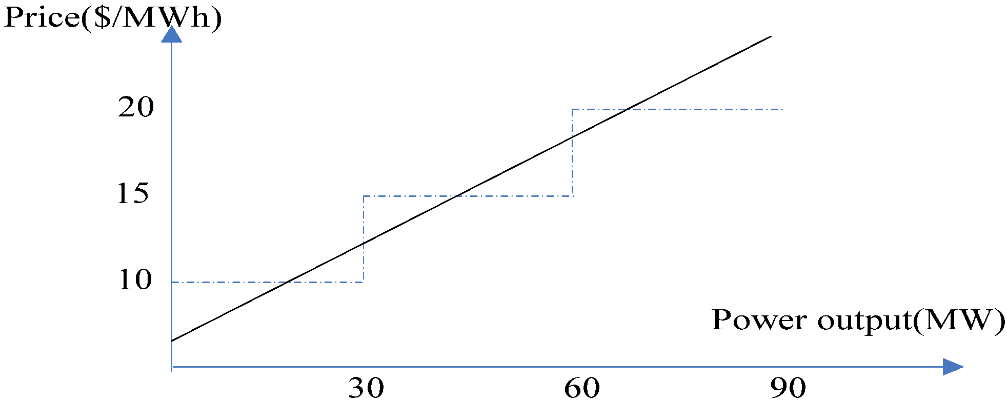
For electricity transactions, The study in [
28] shows that GenCos submit power output in MW (Megawatts) along with associated prices for one bid in both discrete form and continuous form. A bid in discrete form with three different blocks is shown in
Table 1. If the power output level is below 30 MW, the price is 10 $/MWh; If the power output level is between 30 MW and 60 MW, the price is 15 $/MWh; If the power output level is between 60 MW and 90 MW, the price is 20 $/MWh. Generally, this bid could also take a continuous form as shown in
Figure 1. Without loss of generality, a continuous bid curve model is adopted in this paper. For GenCo
i, its bidding curve at time
t is in the form of
pit = α
it + β
itqit, where α
it and β
it are the bidding coefficients of GenCo
i at time
t. Here
pit and
qit respectively, represent the bidding price and the bidding power output of GenCo
i at time
t.
Table 1.
Block bid.
| Blocks | Price ($/MWh) | Power output level (MW) |
|---|
| Block 0 | 10 | 30 |
| Block 1 | 15 | 60 |
| Block 2 | 20 | 90 |
Figure 1.
Block bid and continuous bid curves.
Figure 1.
Block bid and continuous bid curves.
The market clearing price (MCP) is a uniform price shared by all GenCos, and the actual MCP depends on all GenCos’ bidding behaviors. Assume the bidding curve of GenCo
i is
pit = α
it + β
itqit, and the electricity demand at time
t is
Dt. The MCP at time
t, which is denoted as
pt, can be obtained by solving the following power balance equation:
2.1.3. Menu of the Incentive Contracts
The menu of the incentive contracts is composed of multiple contracting terms in the form of (αi, βi, πi), where αi and βi represent the thresholds of bidding coefficients respectively, and πi is the relevant reward for meeting the incentive contract. Though each incentive contract is originally tailored to the rational and incentive-compatibility constraints of a certain target GenCo, it is also expected that these contracts are designed appropriately to motivate non-target GenCos to participate in the incentive program.
Assuming an incentive contract is customized for a target GenCo with bidding coefficients αi0 and βi0, and the amount of the reward is πi0 by calculating the target GenCo’s individual rationality and incentive compatibility conditions. This contract could be expressed by the triplet (αi0, βi0, πi0) which specifies the reward and the obligation associated with the contracted GenCo: if the dispatched power output of the contracted GenCo during the contract period is always greater than the required level, which is prescribed as with pt being the MCP at time t, a reward of πi0 would be received at the end of the contract period.
All sets of (αi, βi, πi) are further incorporated into (AL, B, π), where AL, B, π are the vectors of αi, βi, πi, respectively. Hence the menu of the incentive contracts could be concisely specified in the form of (AL, B, π).
2.2. Scenario-Based Approach
At certain time, unexpected events like hot weather, network congestion, and demand spikes may occur randomly, which causes load soaring and demand forecast errors. Scenario based approach [
16,
29,
30] is often employed to address these types of uncontrollable events. These uncertain events are characterized by scenarios with corresponding probabilities. The scenarios considered in this paper include both normal scenario and bad scenario. In the latter, the load is 20% higher than the average demand. Probability of each scenario could be inferred from historical data and experiences. The Monte Carlo method is adopted to simulate both normal and bad scenarios.
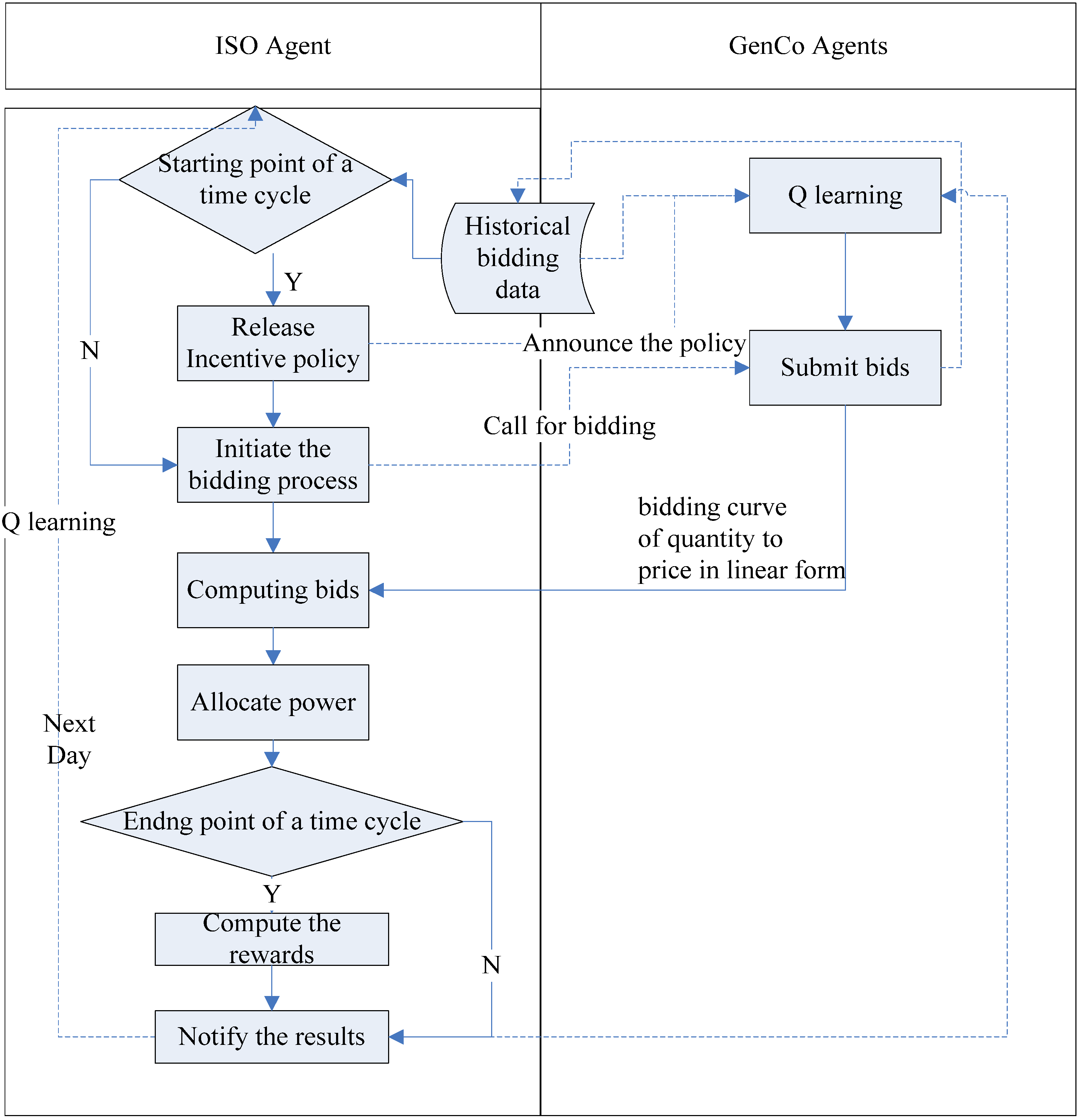
2.3. The Workflow of Multi-Agent System
In this paper, a multi-agent system, adapted to a simulated context with multiple GenCos and one ISO, is proposed to study a day-ahead electricity market based on the proposed incentive menu of contracts. The multi-agent system was developed in a Java platform that was partly inherited from the Repast platform [
31]. Some actions of GenCos were coded by Matlab, and then packaged and implanted into the multi-agent Java platform.
Figure 2 shows the flowchart of multi-agent system (MAS) scheduling procedure.
Figure 2.
Flow chart of multi-agent system (MAS) scheduling mechanism (note: Y = yes and N = no). ISO: independent system operator.
Figure 2.
Flow chart of multi-agent system (MAS) scheduling mechanism (note: Y = yes and N = no). ISO: independent system operator.
At the beginning of a specified period
that consists of
T days (
i.e., a period may include several days, or several months), ISO announces the menu of the incentive contracts. GenCos, which act for their own interest, decide whether they accept the incentive contract or not by using the periodic Q-learning method. This decision-making system resembles the one-leader and multi-followers Stackelberg game where the ISO is the leader and the GenCos are the followers. An algorithm using the idea of the Stackelberg game, which is further illustrated in
Section 4.3, is presented for the ISO to find the initial optimal menu of incentive contracts in the first period. In addition, a periodic Stackelberg-based Q-learning method, which is illustrated in
Section 4.2, is proposed for the ISO to find the subsequent optimal menu of incentive contracts over the following periods.
At the beginning of a period, GenCo i decides whether or not to accept the incentive program, by using its periodic Q-learning method. In each day of the period, GenCo i chooses to place a high bid or a normal bid by using its daily Q-learning method, and submits its bid, taking the form of pit = αit + βitqit. After the ISO receives all the bids from the participants, the relevant information is aggregated and stored in a central repository. Based on the estimated hourly electricity demand of the next day, the ISO decides the unified hourly MCP of the next day, and announces the hourly power output schedule of individual GenCos for the next day.
At the end of period , the ISO computes the relevant rewards based on the bidding data retrieved from the central repository. If any GenCo’s bidding data in the given period are constant, and always in alignment with certain contract in the menu of the incentive contracts, the GenCo would receive the relevant reward. During the repetitive bidding periods, both ISO and the GenCos improve their pricing policy and bidding strategies using the Q-learning algorithm.
3. Multi-Agent Stackelberg Game Model
3.1. Model Assumption and Description
Model assumptions are given as follows:
(1) To prevent GenCos reaping extra profits by modifying their bidding data to satisfy the incentive contract, it is stipulated that any GenCo using new bidding coefficients is not eligible to join the incentive program until after several rounds.
(2) At some time, due to the uncertainties in weather condition, network reliability and consumer behavior, unexpected demand spikes may occur, and the load may vary with a large degree of uncertainty. Probabilistic scenarios trees are adopted to accommodate the uncertain characteristics of the load profile. For instance, the electricity demand at time t is estimated to be 100 MW with probability of 0.8 for the normal demand scenario, and 150 MW with probability 0.2 for the high demand scenario, or bad scenario. Enumeration methods can be used to capture all possible scenarios if the problem size is not too large. Let Λ denote a set of uncertain scenarios, and λt denotes a realized scenario in Λ at time t. In addition, ΛB is used to represent a set of bad scenarios.
(3) It is assumed that each GenCo within the MAS framework have two bidding options: either place a high bid (
i.e.,
bi,t = 1) or place a normal bid (
i.e.,
bi,t = 0), where
bi,t is the bidding strategy of GenCo
i at time
t. The coefficients for different bidding options are defined as follows:
where α
ic, β
ic are parameters of the normal bidding curve for GenCo
i, and α
ih, β
ih are parameters of the corresponding high bidding curve. Obviously, if a GenCo has accepted an incentive contract, we have
bit = 0, α
i,t = α
ic, β
i,t = β
ic for
.
3.2. Single-Period Decision-Making Model of GenCo
Based on the given menu of incentive contracts, in each time period, a GenCo tries to maximize its profit by choosing the best bidding strategy as follows:
For a GenCo who does not accept any incentive contract, its profit is given as:
where
, and
ρ(λ
t) represents the probability of λ
t, and
is the reward specified in the incentive contract for target GenCo
k.
It is usually difficult for a GenCo to know the actual bidding behavior of others, but it is reasonable to assume that the probability of its competitors’ decision can be inferred from historical data. Hence
can be obtained as:
where:
where
is the power output of GenCo
i when its bidding action is
bi,t in a scenario λ
t.
ci1 and
ci2 are cost coefficients of GenCo
i.
bti,c = {
b1,t,
b2,t,
bi-1,t, 0,
bi+1,t,…,
bm,t} represent a bidding combination when GenCo
i places a normal bid. Note that
posj(
bj,t) is the probability for GenCo
j to take action
bj,t. Here
p(λ
t,
bt(
a)) is the expected electricity price when the bidding combination of GenCos is
bt(
a) in scenario λ
t. Note that
p(λ
t,
bt(
a)) is
p(λ
t,
bti,C) when GenCos’ bidding action is
bti,C in scenario λ
t, and is
p(λ
t,
bti,H) when GenCos’ bidding action is
bti,H in scenario λ
t.
For a contracted GenCo who agrees on the acceptance of an incentive contract which is tailored to the target GenCo
k, its profit could be calculated as follows:
Assuming the incentive contract is prescribed as (α
k, β
k, π
k) triplet, we have:
So
could be calculated as:
subject to:
The optimization problem faced by a GenCo is how to choose an optimal bidding strategy such that its expected profit is maximized. Hence the incentive-compatibility constraint could be formulated as:
If a GenCo accepts an incentive contract, its expected profit should be higher than the alternative. Thus the personal rationality constraint could be re-formulated as:
3.3. Optimization Problem of Independent System Operator
From the ISO’s point of view, its goal is to design an optimal menu of incentive contracts such that the average MCP during the period remains at a relatively stable level, or the volatility of price in the worst scenarios could be mitigated, while the total electricity payment is minimized. To that end, it is necessary for the ISO to identify the optimal set of target GenCos (i.e., a0) as well as designing the incentive menu for attracting contracted GenCos, so that its objectives could be optimized. Since an incentive contract, which is specified in the triplet form of (αi, βi, πi), is dependent upon a0, how to target suitable GenCos is the key to designing an optimal incentive menu of contracts. Hence the ISO’s initial decision is to choose optimal a0, so as to minimize the total cost with certain price stability.
As the leader of the Stackelberg game, the ISO can analyze the response of the followers (
i.e., GenCos) so as to find the optimal decision variable
a0. A two-level programming model is proposed to facilitate ISO’s decision-making. The sub-problem at the first level enables the ISO to minimize the total cost with price stability by finding an optimal value of
a0. The sub-problem at the second level can be treated as GenCos’ reaction model upon the release of the menu of incentive contracts from the first level decision:
subject to:
where
ai is obtained by solving follows:
where
C(
a0) is the total power purchasing cost when the combination of the target GenCos is
a0, and
is a balance parameter. EP(
a0) is the expected electricity price when the combination of the target GenCos is
a0, and EP
* is the best expected price. BP(
a0) is the variance of mean price
versus EP
* when the combination of the target GenCos is
a0. Here
P(λ
t,
a) is the expected MCP when the combination of contracted GenCos’ is
a in scenario λ
t. The MCP is
p(λ
t,
bt(
a)) when the bidding behavior of GenCos is
bt(
a) in scenario λ
t.
As shown in Equation (19), one of the ISO’s objectives is to minimize the electricity payment. Equation (20) is another objective of the ISO, that contains dual goals: Firstly, minimizing the common price in the contract period; and secondly minimizing the volatility of price. Both goals are combined by a balance factor. Equation (21) indicates that a is also decided by a0. Equations (22) and (23) are the mathematical descriptions of the cost and the reward, respectively. Equation (24) calculates the average price in one period under multiple scenarios. Equation (25) calculates the variation of mean price versus EP* in one period in multiple scenarios. Equation (26) ensures that the electricity demand is always satisfied. Equation (27) computes the average price by multiplying the price for certain bid combination in a specified scenario with its occurrence possibility. Equations (28)–(30) provide the mathematical descriptions for , , , respectively. Equation (31) represents the GenCos’ objective which is also their incentive-compatibility constraint with ai being the decision variable for GenCo i. Equation (32) gives the personal rational constraint of the GenCos who is willing to accept an incentive contract. Finally, Equations (33)–(35) defines the constraints of contracted GenCos including power output capacity of contracted GenCos, and the possibilities of contracted GenCos to place high bids or normal bids.
A multi-objective optimization can be solved by turning it into a single objective model through appropriately assigning weight to each objective function. Using a weight
w to combine the two objectives in Equations (19) and (20), the ISO’s decision model could be further expressed as:
subject to:
where
ai is obtained by solving follows:
where
Cmax is the maximum available
C(
a0);
Cmin is the minimum available
C(
a0); EPM(
a0) is a balance between price minimization and price variation minimization when the decision variable is
a0 . EPM
max is the maximum available EPM(
a0); and EPM
min is the minimum available EPM(
a0). Equations (38)–(52) are the same with Equations (21)–(35).
4. Q-Learning for Agents’ Optimal Decision Making
Each agent interacts in the volatile market environment due to the uncertain load and lack of precise knowledge of its competitors. It is imperative for the agents to evolve their actions through the learning of repeated bidding processes. Q-learning is one of the reinforcement learning methods, and could guide the agents to improve the performance of their decision making over time. In each period, an agent perceives the state of the market environment, and takes certain actions based on its perception and past experience, which result in a new state. This sequential learning process would reinforce its subsequent actions. Quite a few studies have been done on Q-learning, and its application in the electricity market has been reported. For instance, Rahimiyan and Mashhadi [
32] propose a fuzzy Q-learning method to model the GenCos’ strategic bidding behavior in a competitive market condition, and find that GenCos could accumulate more profit by using fuzzy Q-learning. Naghibi-Sistani
et al. [
33] developed a modified reinforcement learning based on temperature variation, and applied it to the electricity market to determine the GenCos’ optimal strategies. Attempts also have been made to combine the Q-learning with Nash-Stackelberg games for reaching a long-run equilibrium. Haddad
et al. [
34] incorporate a Nash-Stackelberg fuzzy Q-learning into a hierarchical and distributed learning framework for decision-making, with which mobile users are guided to enter the equilibrium state that optimizes the utilities of all the network participants.
In this paper, Q-learning methods are adopted by ISO and GenCos for the making decisions. Different learning algorithms are designed for ISO and GenCos because they have different goals. For GenCos, both a periodic Q-learning method and a daily Q-learning method are applied to the bidding decision process. For ISO, a Stackelberg-based Q-learning is adopted to design the menu of incentive contracts in each period.
4.1. Periodic and Daily Q-Learning Methods for Generating Companies
At the starting point of a period, a GenCo decides whether the incentive contract should be accepted or declined. In each day of the period, the GenCo should choose to place a high bid or place a normal bid. Especially, if a contracted GenCo decides to place a high bid, the reward at the end of the period, would be cancelled. To calculate the potential reward, a multi-step Q-learning method is adopted by the GenCo to decide its bidding strategy in daily basis. Two Q-learning methods are proposed for the GenCo’s periodic and daily decision making. The state, actions, reward and Q-value function are defined as follows:
4.1.1. State Identification
State is defined for GenCo’s Q-learning method for a period, and it is composed of values of all possible average electricity prices over one period.
State denote the states for GenCo’s Q-learning method in each day, and it is composed of values of all possible average electricity prices over one day.
4.1.2. Action Selection
Let a discrete set of actions , denote the action selection of GenCo i at the starting point of a period for GenCo’s Q-learning method for a period. When = 0, GenCo i chooses not to accept the incentive contract over period . When , GenCo i accepts the incentive contract which is tailored to the target GenCo k over period .
denotes the action selection of GenCo i in each day for GenCo’s Q-learning method for a day, and its value is 0 or 1. When , GenCo i adopts a normal bidding strategy; When , GenCo i adopts a high bidding strategy.
When , in each day of the period , GenCo i places a normal bidding strategy. So for a contracted GenCo, , with a high probability.
4.1.3. Reward Calculation
The periodic reward function for Q-learning method over period
is defined as:
Equation (53) represents the reward assigned to action from the old state . If = 0, which means that the menu of incentive contracts is not accepted over period , . If , which means that GenCo i accepts the incentive contract which is tailored to the target GenCo k over period , an amount of is received as the reward for meeting the incentive contract. The reward would further influence the periodic Q-value which guides the GenCo to determines the next action as whether or not to accept the incentive menu.
Every day the GenCo agent evaluates the current state, and chooses the best action that optimizes its objectives. Then the current state evolves to the new state, with a transition probability, and the agent receives a reward.
The reward
r for daily Q-learning is made up of two parts. One is the direct profit subject to all the GenCo agents’ bidding behaviors, loads, and cost of the GenCo agent. The second is a portion of the expected reward if the GenCo accepts the incentive contract. If a GenCo agent accepts the incentive menu and fulfills the contractual obligations in the contract period, a reward would be obtained at the end of the period, so the reward is a delayed reward. A multi-step reward function, which captures the characteristic of the delayed reward, is defined to describe GenCo agent’s daily Q-learning as follows:
subject to:
where,
where
is a discount factor, and
is the reward for GenCo
i to meet the incentive contract terms at time
t, and
T is the total number of days in a contract period, and
Ts is the number of the days elapsed in the period.
4.1.4. Q-Value Update
By Q-learning, using the Bellman optimality in Equations (57) and (58), each GenCo agent tries to find the optimal action to maximize the Q-value of each state in a long run.
The periodic Q-value function defined for GenCo
i over period
is given as follows:
where
is a positive learning rate at period
, and
is a discount parameter at period
.
These action-state value functions
(
i = 1, ...
m), which are greatly affected by the reward function as illustrated in Equation (53), determine the GenCo agents’ most suitable actions for the next run. That is, if the Q-value for accepting the incentive menu is less than the Q-value for not accepting it, the GenCo agent would not take the action of accepting the incentive menu. Conversely, it would. The daily Q-value function defined for GenCo
i at each day is given as follows:
where
is a positive learning rate in day
t, and
is a discount parameter in day
t. 4.2. Q-Learning for the Leader of the Stackelberg Game (Independent System Operator)
4.2.1. State Identification
State for ISO’s Q-learning is composed of two state variables, one is the values of all possible average electricity prices during that period, and the other is the decision variable for menu of the incentive contracts.
4.2.2. Action Selection
The set of all possible combinations of target GenCos, or A0 is defined as the set of action selection of ISO agent. The ISO takes the action at each step, or at the starting point of each period. denotes the action selection of ISO in period .
4.2.3. Reward Calculation
Reward function
is given by:
Equations (59)–(61) illustrates that , which is the GenCo i’s action in period t, depends on its Q-learning, and so the reward of the ISO is obtained by using a Stackelberg-based Q-learning method.
4.2.4. Q-Value Update
As the leader of the Stackelberg game, Q-learning algorithm for ISO is given as follows:
4.3. Solution Methodology for Independent System Operator’s Initial Q Value
For problems with multiple decision variables, chaos search is more capable of hill-climbing and escaping from the local optima than the random search [
35]. Hence a chaos optimization algorithm is proposed to solve the problem
The detailed procedure of the algorithm is given as follows:
- Step 1:
set initial parameters incorporating bidding coefficients of GenCos and its power capacity.
- Step 2:
set .
- Step 3:
generate a non-zero chaos variable
using cube mapping method as shown below:
- Step 4:
decoding the chaos variables into a binary variable which represents a value for the sets of target GenCos.
- Step 5:
calculate the tailoring values of (αi, βi, πi) for all target GenCos using Equation (18).
- Step 6:
for the designed menu of the incentive contracts, check each GenCo’s optimal reaction by solving Equation (17).
- Step 7:
calculate the corresponding objective value and the state for ISO’s Q-learning. The latter includes the mean electricity price during the period, and the menu of the incentive contracts. If the obtained objective value is larger than the existing one, substitute the existing one.
- Step 8:
substitute the chaos variables into Equation (64) to yield new chaos variables:
where
and
are two constant vectors, and
is the integr part of
.
- Step 9:
Set , k = k + 1.
- Step 10:
If , stop searching, else go to Step 4.
5. Simulations and Analysis
The simulation is performed in a day-ahead electricity market with the participation of five GenCos. The original probability for a GenCo to bid high or normal is 0.5. Electricity demand at each hour varies between 170 MW and 230 MW. The probability of high-demand scenarios, which are also termed as bad scenarios, is less than 0.2. The length of a contract could be several days, or a couple of months. For computational convenience, firstly it is assumed that each period consists of seven days or one week.
Parameters of GenCos’ bidding curves are listed in
Table 2, and the GenCos’ cost parameters are listed in
Table 3, and the weights of the two objectives are listed in
Table 4. Three cases are investigated for the comparative analysis.
- Case 1:
no menu of incentive contracts or Q-learning.
- Case 2:
menu of incentive contracts without Q-learning in one period. Eight sub-cases are further analyzed, and the comparative results are listed in
Table 5 and
Table 6.
- Case 3:
menu of incentive contracts with Q-learning in multiple periods. Note that load demand over the multiple periods varies between 170 MW and 230 MW.
Table 2.
Parameters of GenCos’ bidding curves. (Unit for αi,tc, αi,th: $/MW per hour, unit for βi,tc, βi,th: $/(MW)2 per hour).
Table 2.
Parameters of GenCos’ bidding curves. (Unit for αi,tc, αi,th: $/MW per hour, unit for βi,tc, βi,th: $/(MW)2 per hour).
| GenCo No. | Case 1, Cases 2.1–2.5, Case 3 | Cases 2.6–2.8 |
|---|
| αi,tc | βi,tc | αi,th | βi,th | αi,tc | βi,tc | αi,th | βi,th |
|---|
| 1 | 10 | 0.5 | 10.5 | 0.525 | 10 | 0.5 | 10.5 | 0.525 |
| 2 | 11 | 0.8 | 12 | 0.84 | 11 | 0.8 | 12 | 0.84 |
| 3 | 8 | 0.6 | 8.4 | 0.63 | 8 | 0.9 | 8.4 | 0.945 |
| 4 | 15 | 0.5 | 15.75 | 0.525 | 15 | 0.5 | 15.75 | 0.525 |
| 5 | 20 | 0.9 | 21 | 0.945 | 20 | 0.6 | 21 | 0.63 |
Table 3.
GenCos’ cost parameters. (Unit for ci1: $/MW, unit for ci2: $/(MW)2).
Table 3.
GenCos’ cost parameters. (Unit for ci1: $/MW, unit for ci2: $/(MW)2).
| GenCo No. | Cases 2.1–2.4 and 2.6–2.8 | Case 2.5 |
|---|
| ci1 | ci2 | ci1 | ci2 |
|---|
| 1 | 10 | 0.5 | 5 | 0.25 |
| 2 | 11 | 0.55 | 6 | 0.35 |
| 3 | 8 | 0.5 | 4 | 0.25 |
| 4 | 15 | 0.8 | 7 | 0.4 |
| 5 | 20 | 0.9 | 10 | 0.45 |
Table 4.
Objectives of Cases 2.1–2.8.
Table 4.
Objectives of Cases 2.1–2.8.
| Cases | Cost | EPM (0.5 × EP + 0.5 × BP) |
|---|
| 2.1, 2.5, 2.6 | 1 | 0 |
| 2.2, 2.7 | 0 | 1 |
| 2.3, 2.8, 3 | 0.5 | 0.5 |
| 2.4 | Without menu of incentive contracts |
Table 5.
Comparative results for Cases 2.1–2.3 and 2.5 (unit: $,). (Note: Y = saying “Yes” to offer of the incentive contract menu and N = saying “No” to the offer).
Table 5.
Comparative results for Cases 2.1–2.3 and 2.5 (unit: $,). (Note: Y = saying “Yes” to offer of the incentive contract menu and N = saying “No” to the offer).
| Items | Case 2.1 | Cases 2.2 and 2.3 | Case 2.5 |
|---|
| Target GenCos | 1 | 0 | 0 | 0 | 1 | 1 | 0 | 0 | 1 | 1 | 0 | 1 | 0 | 1 | 1 |
| GenCos’ response | Y | Y | Y | N | Y | Y | Y | Y | Y | Y | Y | Y | Y | Y | Y |
| Expected reward | 208,750 | 543,530 | 123,070 |
| Expected cost saving (compared with Case 2.4) | 597,830 | 512,120 | 932,580 |
| Expected price (EP) | 37.17 | 36.94 | 36.94 |
| BP (mean price variance in bad scenarios) | 2.78 | 2.53 | 2.53 |
| EPM (0.5 × EP + 0.5 × BP) | 19.97 | 19.74 | 19.74 |
Table 6.
Comparative results for Cases 2.6–2.8 (unit: $, N/A = Not Applicable).
Table 6.
Comparative results for Cases 2.6–2.8 (unit: $, N/A = Not Applicable).
| Items | Case 2.6 | Cases 2.7 and 2.8 |
|---|
| Target GenCos | 0 | 0 | 1 | 0 | 1 | 0 | 0 | 1 | 1 | 1 |
| GenCos’ response | Y | Y | Y | N | Y | Y | Y | Y | Y | Y |
| Expected reward | 215,980 | 581,130 |
| Expected cost saving (compared with Case 2.9) | 607,780 | 497,270 |
| EP | 38 | 36.94 |
| BP (meanprice variance in bad scenarios) | 2.78 | 2.53 |
| EPM (0.5 × EP + 0.5 × BP) | 20.39 | 20.15 |
| Threshold for GenCo’s power output | 1 | 6558 | 6477 |
| 2 | 7145 | 7091 |
| 3 | 7145 | 7091 |
| 4 | N/A | 9852 |
| 5 | 6558 | 6477 |
Case 2.1 aims at minimizing cost. Cost in Case 2.1 is less than that in Cases 2.2 and 2.3, but EP and BP in Case 2.1 are larger compared with that in Cases 2.1 and 2.3.
In Case 2.5, though it also aims at minimizing cost, as GenCos have small cost coefficient, they could gain more profits compared with Cases 2.1–2.4, and so GenCos in Case 2.5 prefer to make normal bids since they could obtain more power output and hence more profit, and so both cost and EPM could be minimized.
Since GenCo 3 has higher bidding coefficients in Cases 2.6–2.8, it has more influence on MCP than in Cases 2.1–2.5. Hence GenCo 3 is more likely to be the target GenCo in Cases 2.6–2.8 than in Cases 2.1–2.5.
Figure 3 and
Figure 4 show the simulation results of variations in price and cost across 112 days in Cases 1 and 3.
Figure 3.
Comparative results of price variation for Cases 1 and 3 (for 112 days).
Figure 3.
Comparative results of price variation for Cases 1 and 3 (for 112 days).
It can be seen that the variations of electricity price and cost could be reduced in the long term provided that the incentive contract is adopted. It could be seen that in the early phases, the effect of the incentive contract is not obvious as the daily price and daily electricity purchase cost do not significantly decrease in Case 3. However, as time evolves, GenCos can enhance their bidding experience through learning from past bidding processes and realize that accepting the incentive contract could help improve their profitability. They become more interested in participating in the incentive program. As a result, the electricity price is kept at a low and stable level.
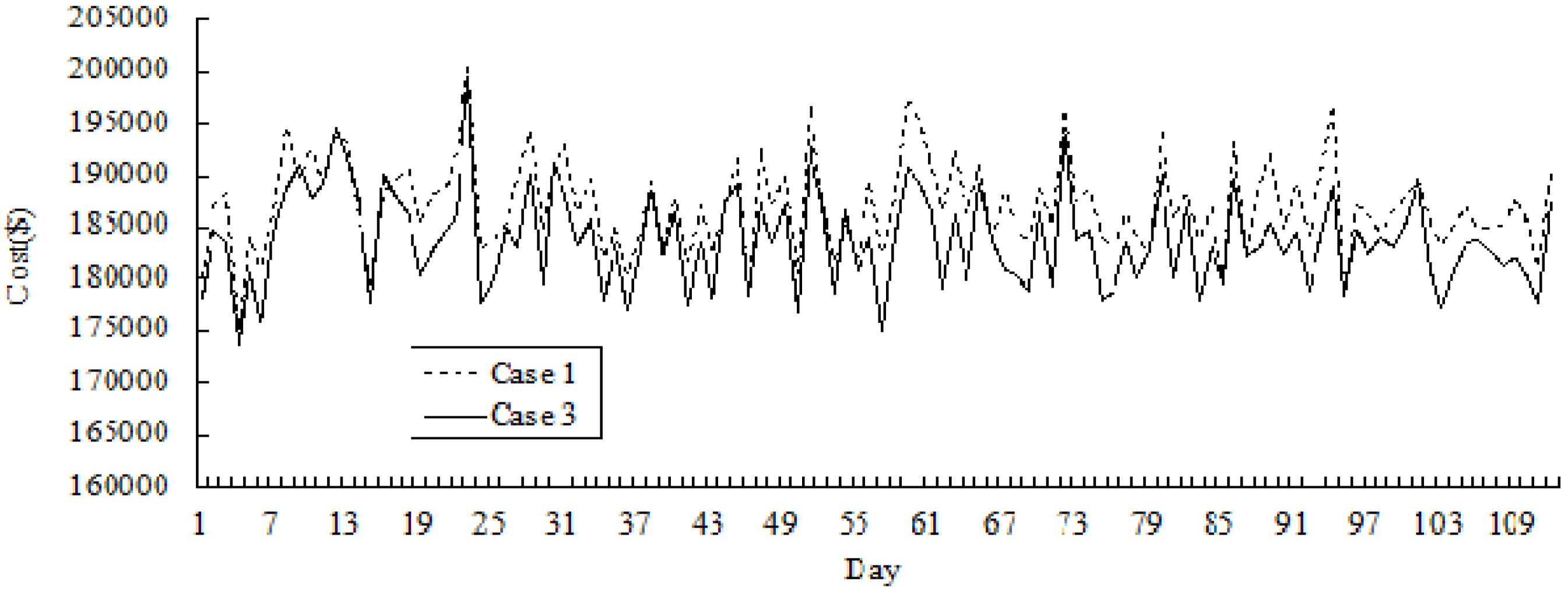
Figure 4.
Comparative results of cost variation for Cases 1 and 3 (for 112 days).
Figure 4.
Comparative results of cost variation for Cases 1 and 3 (for 112 days).
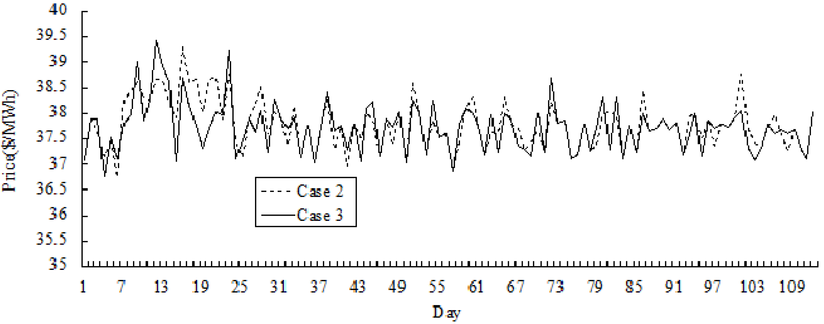
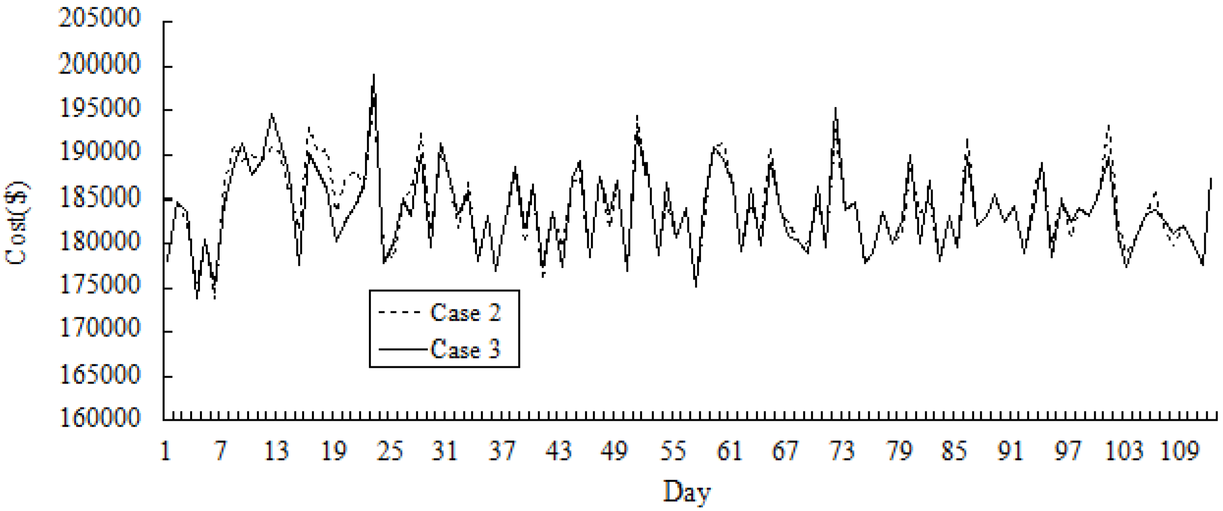
Figure 5 and
Figure 6 show the simulation results of the variations of price and the cost across 112 days in Cases 2 and 3. It could be seen that in the early periods, the cost in Case 3 may be higher than that in Case 2 over certain number of days, and the price in Case 3 is higher than that in Case 2. As GenCos and ISO accumulate more bidding experiences by Q-learning, optimum decisions in Case 3 could be made by both players, and the cost and the price could be reduced compared with that in Case 2.
Figure 5.
Comparative results of price variation for Cases 2 and 3 (for 112 days).
Figure 5.
Comparative results of price variation for Cases 2 and 3 (for 112 days).
Figure 6.
Comparative results of cost variation for Cases 2 and 3 (for 112 days).
Figure 6.
Comparative results of cost variation for Cases 2 and 3 (for 112 days).
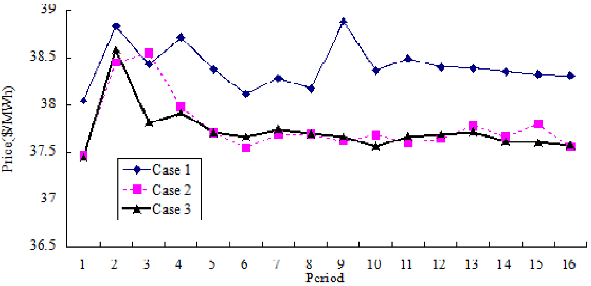
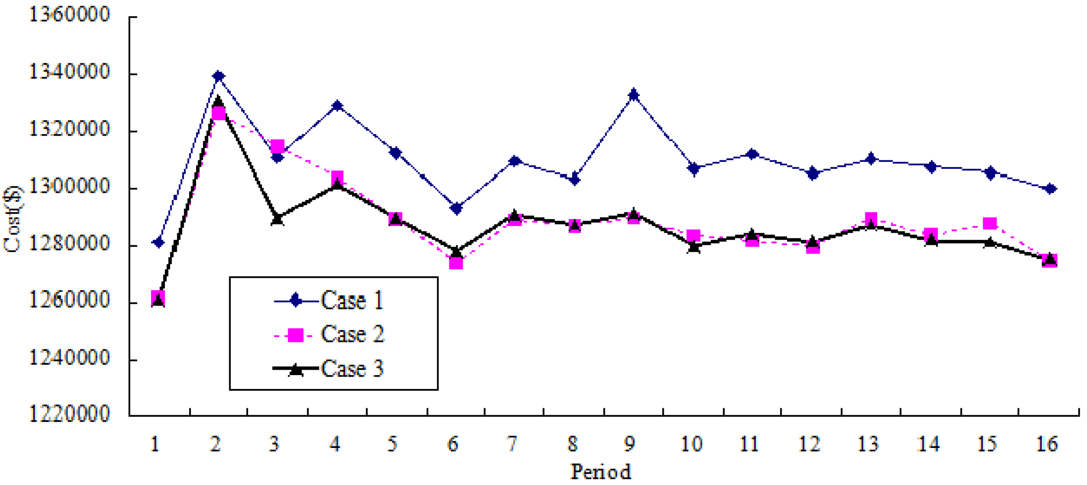
Figure 7 and
Figure 8 show the comparative results of average price variation and average cost variation for three cases, respectively. Based on Case 3, it could be seen that both the cost and the price could be reduced and remain stable in a long run.
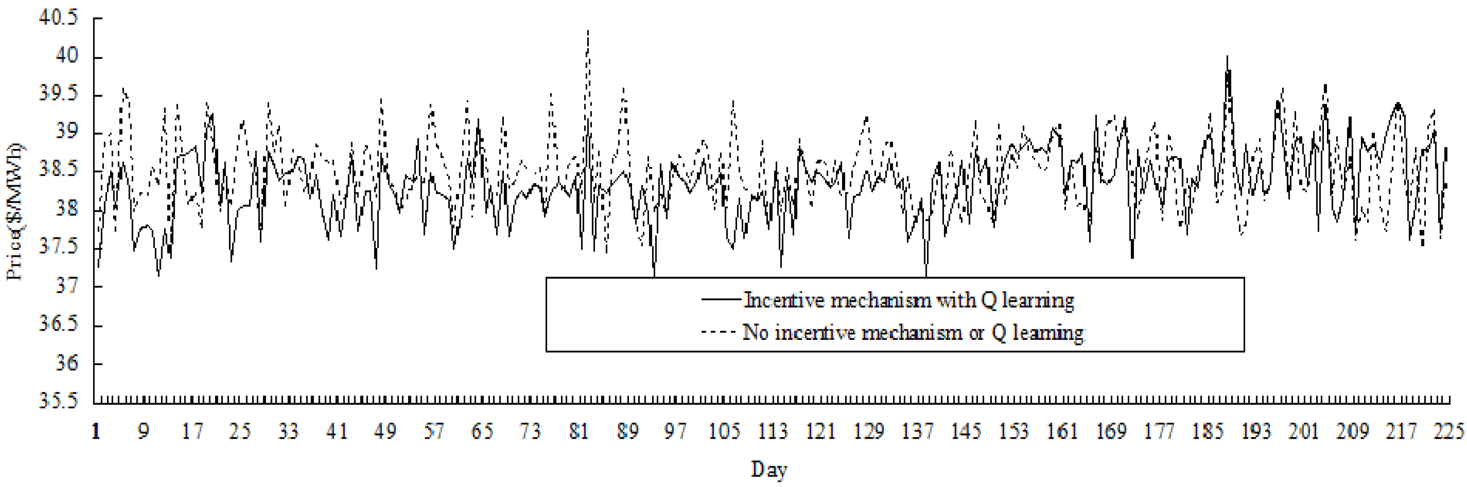
Extending the length of the contract period to 14 days, the comparative results for the duration of 224 days (
i.e., 16 periods) are shown in
Figure 9, and it could be seen that price variation in the electricity market with incentive mechanism is less than the market without incentive mechanism. In fact, the price variance in the former market is 0.242
versus 0.270 in the latter, and the average price in the former market is 38.33
versus 38.50 in the latter (price unit is $/MWh).
Figure 7.
Comparative results of average price variation for 3 Cases (for 16 periods).
Figure 7.
Comparative results of average price variation for 3 Cases (for 16 periods).
Figure 8.
Comparative results of average cost variation (for 16 periods).
Figure 8.
Comparative results of average cost variation (for 16 periods).
Figure 9.
Comparative results of price variation (for 224 days).
Figure 9.
Comparative results of price variation (for 224 days).
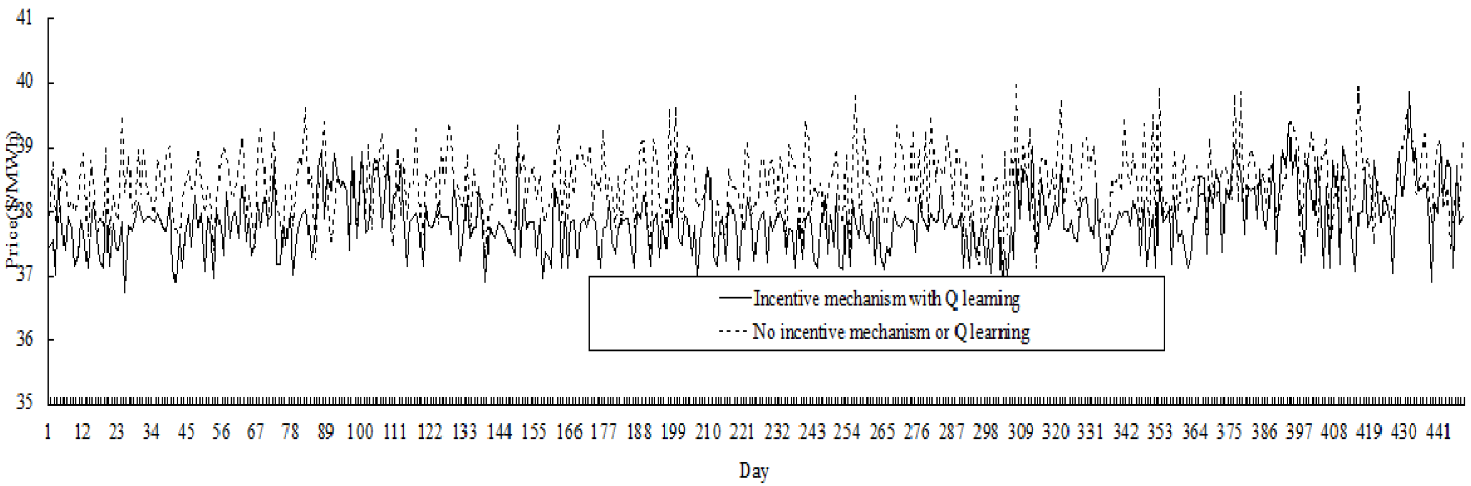
Extending the single contract period to 28 days, the comparative results for 448 days (
i.e., 16 periods) are shown in
Figure 10. It could be seen that price variation in the electricity market with incentive mechanism is less than the market without incentive mechanism. In fact, the price variance in the former market is 0.252
versus 0.310 in the latter, and the average price in the former market is 37.86
versus 38.43 in the latter (price unit is $/MWh).
Figure 10.
Comparative results of price variation (for 448 days).
Figure 10.
Comparative results of price variation (for 448 days).


