
Gas Turbine Transient Performance Tracking Using Data Fusion Based on an Adaptive Particle Filter


Abstract
:
1. Introduction
2. Problem Formulation and Particle Filter
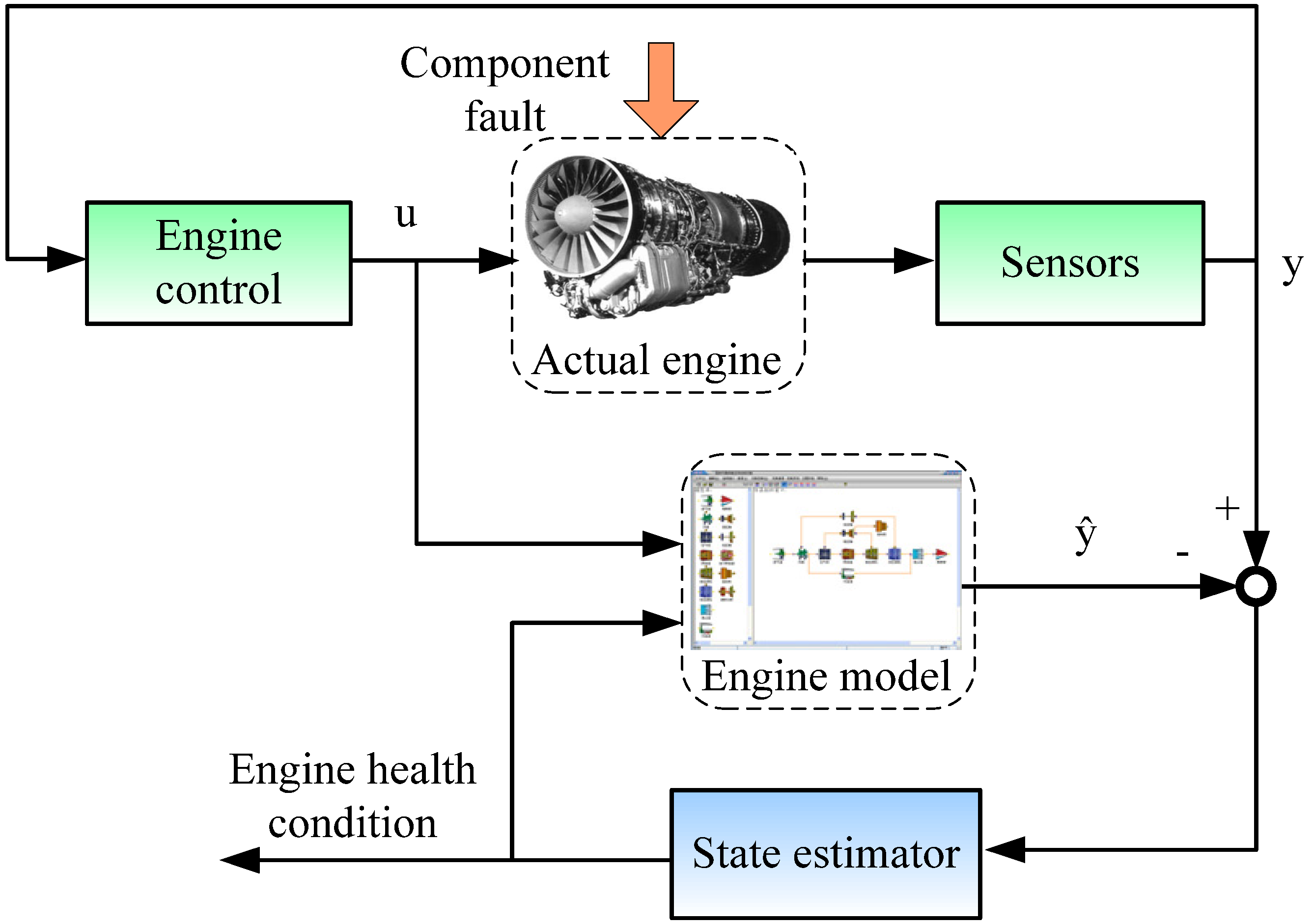
2.1. Problem Formulation

2.2. The Particle Filter
3. Adaptive Fusion Particle Filter
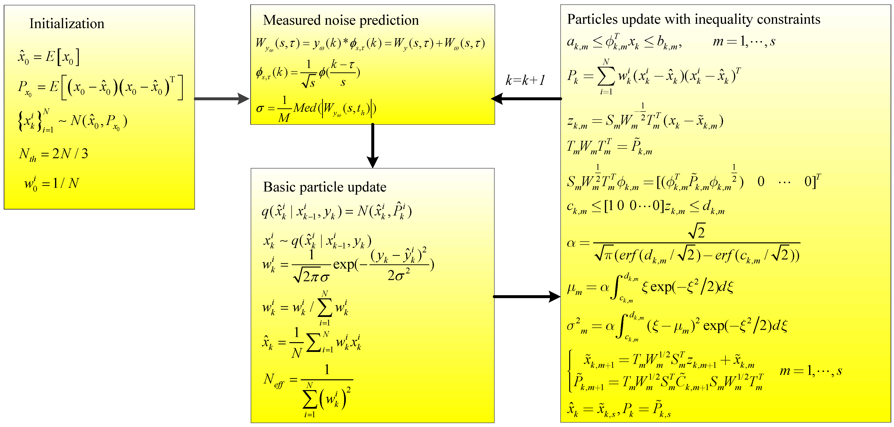
3.1. The Adaptive Particle Filter
3.1.1. Particle Filter with Inequality Constraints
3.1.2. Measure Noise Tuned Particle Filter
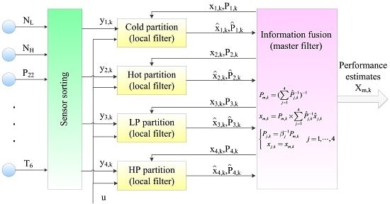
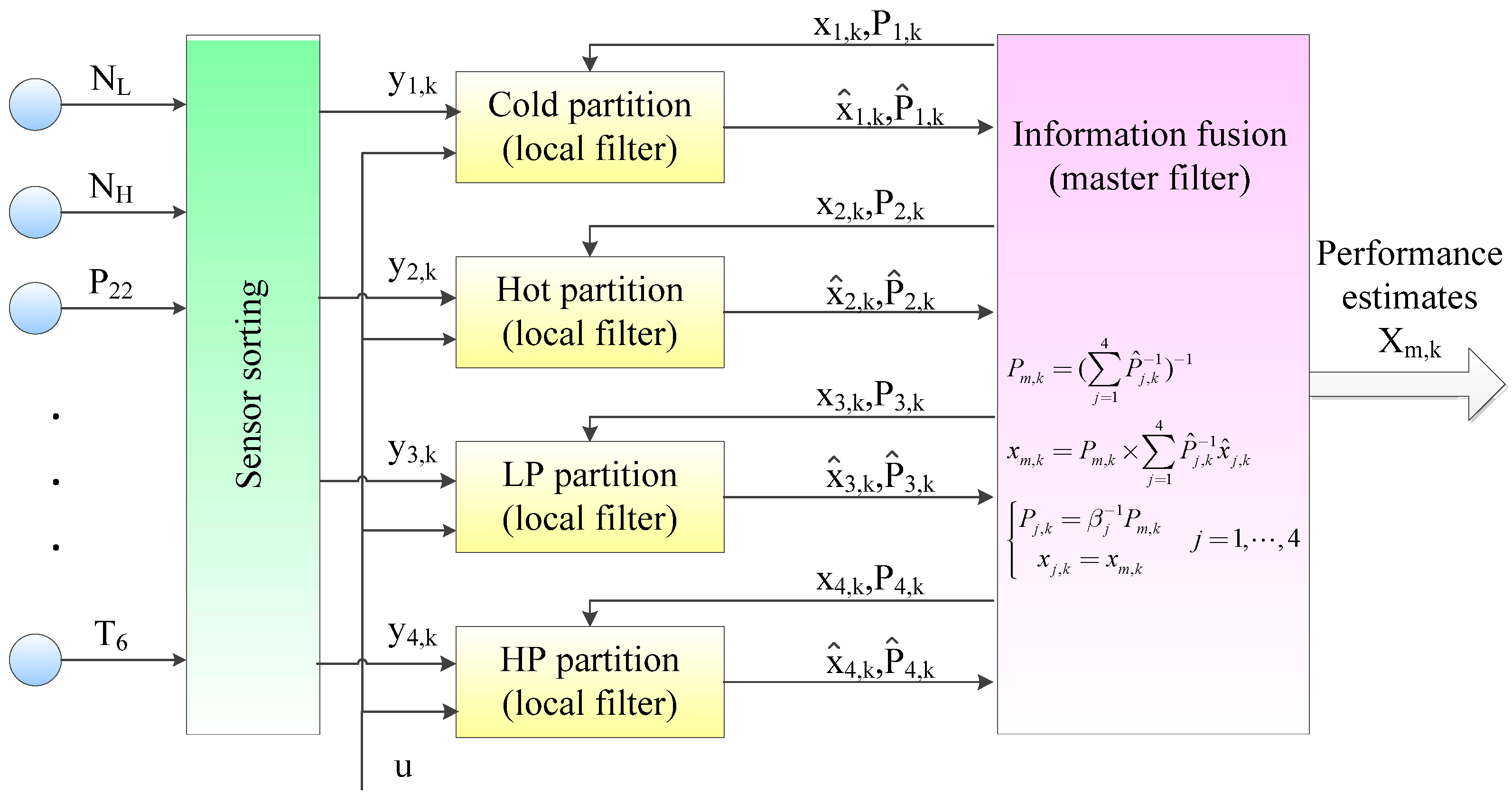
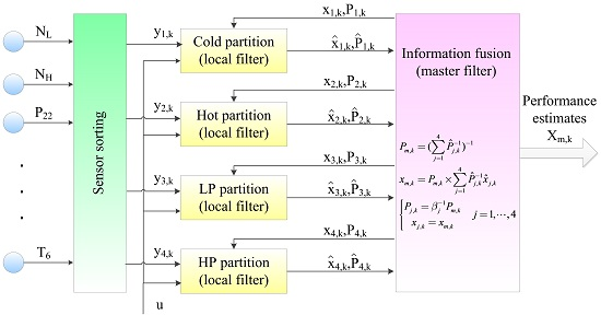
3.2. Data Fusion Based on Adaptive Particle Filter
Step 1: Initialization
Step 2: The adaptive PF performs in the local filter.
Step 3: Information fusion implements in the master filter.
Step 4: Information distribution strategy
4. Simulation and Analysis

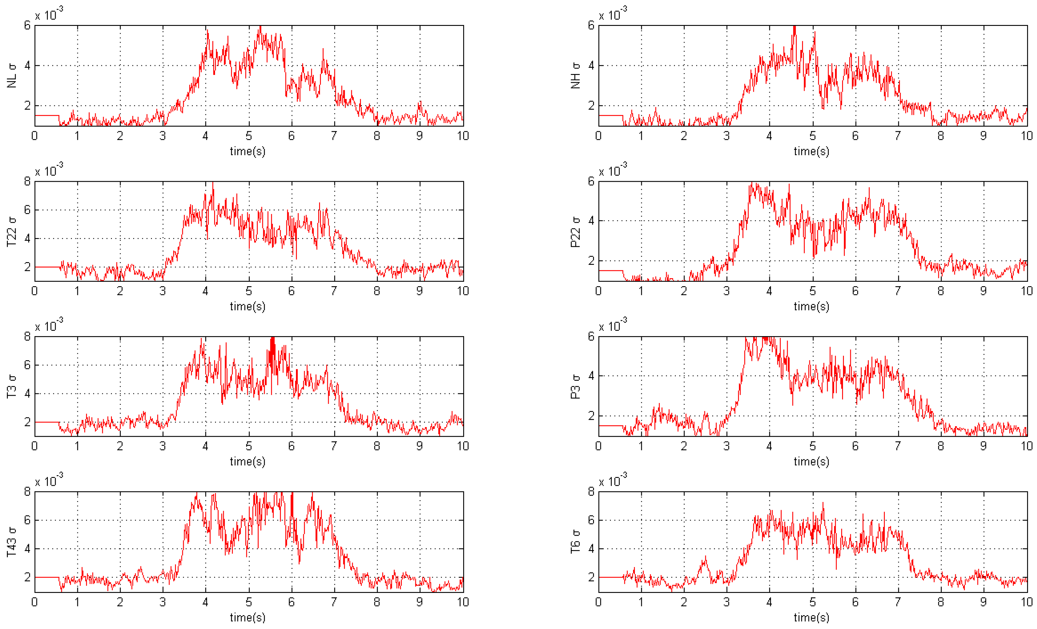
| Measurement | Acronyms | Normalized Value | Standard Deviation |
|---|---|---|---|
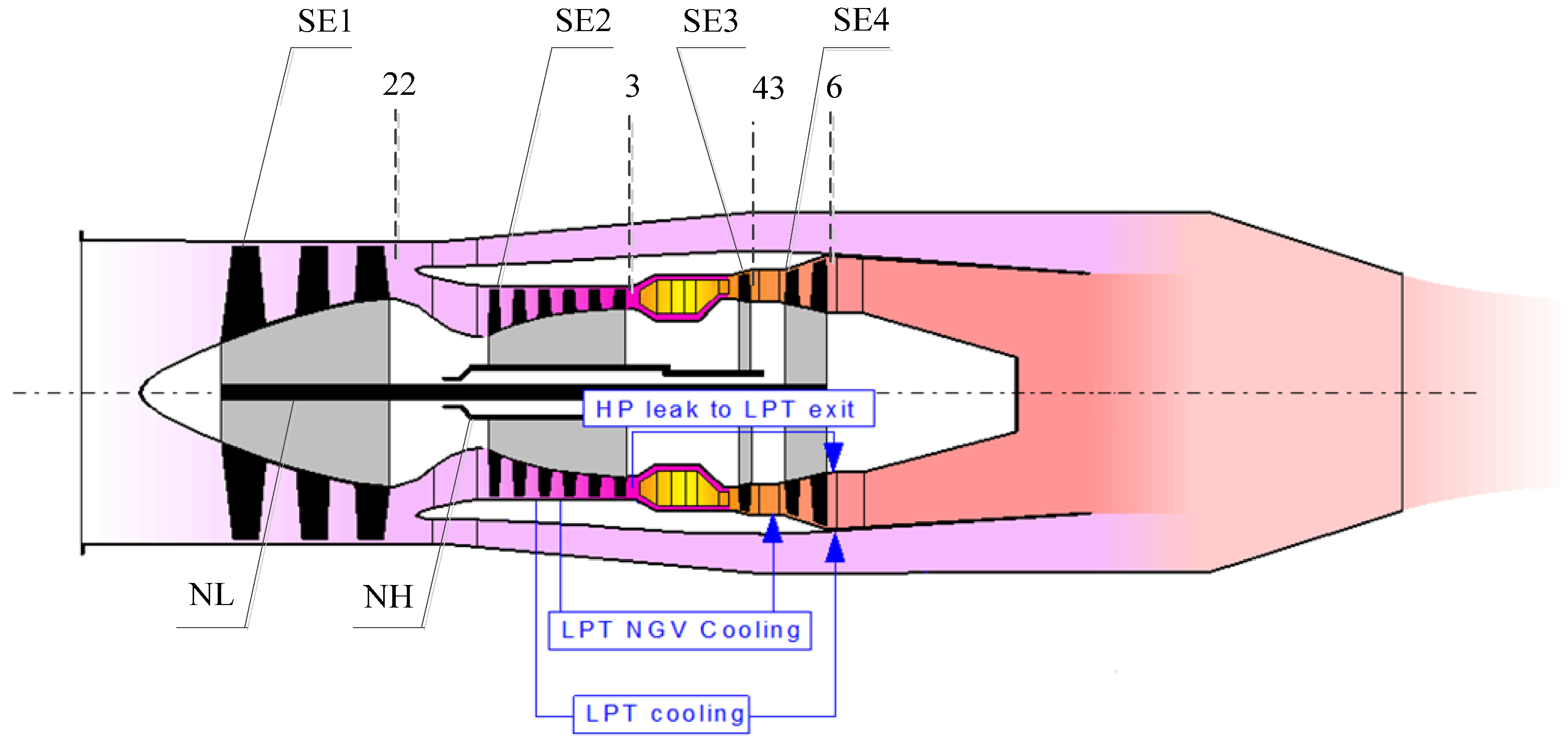
| Low pressure spool speed | NL | 1 | 0.0015 |
| High pressure spool speed | NH | 1 | 0.0015 |
| Fan outlet temperature | T22 | 1 | 0.002 |
| Fan outlet pressure | P22 | 1 | 0.0015 |
| HPC outlet temperature | T3 | 1 | 0.002 |
| HPC outlet pressure | P3 | 1 | 0.0015 |
| HPT outlet temperature | T43 | 1 | 0.002 |
| LPT outlet temperature | T6 | 1 | 0.002 |
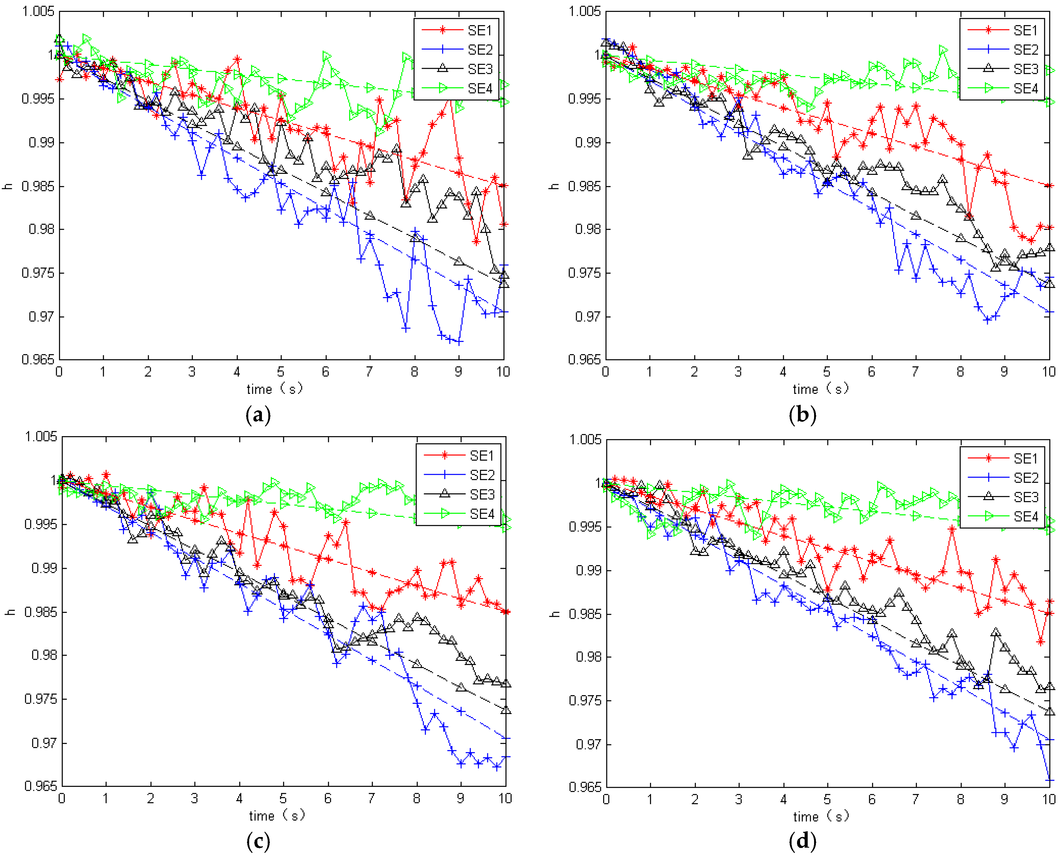
| Scenarios | Acronyms | Fault Mode | Deviation | Standard Deviation |
|---|---|---|---|---|
| Case 1 | SE1 | Fan abrupt fault | −1% on SE1 | 0.0005 |
| Case 2 | SE2 | HPC abrupt fault | −1% on SE2 | 0.0005 |
| Case 3 | SE3 | HPT abrupt fault | −1% on SE3 | 0.0005 |
| Case 4 | SE4 | LPT abrupt fault | −1% on SE4 | 0.0005 |
4.1. Abrupt Fault Diagnosis in Steady Operation Conditions
| Fault Modes | Root-Mean-Square Error (RMSE) | Root-Mean-Square Deviation (RMSD) | Tc (ms) | |||||||||
|---|---|---|---|---|---|---|---|---|---|---|---|---|
| KF | PF | F-PF | FA-PF | KF | PF | F-PF | FA-PF | KF | PF | F-PF | FA-PF | |
| Case 1 | 0.0141 | 0.0108 | 0.0073 | 0.0059 | 0.0090 | 0.0085 | 0.0052 | 0.0044 | 220 | 190 | 230 | 220 |
| Case 2 | 0.0137 | 0.0111 | 0.0078 | 0.0057 | 0.0094 | 0.0089 | 0.0059 | 0.0047 | 260 | 440 | 420 | 440 |
| Case 3 | 0.0113 | 0.0118 | 0.0087 | 0.0060 | 0.0093 | 0.0096 | 0.0061 | 0.0050 | 320 | 620 | 660 | 600 |
| Case 4 | 0.0126 | 0.0115 | 0.0080 | 0.0067 | 0.0100 | 0.0091 | 0.0058 | 0.0051 | 460 | 680 | 760 | 640 |
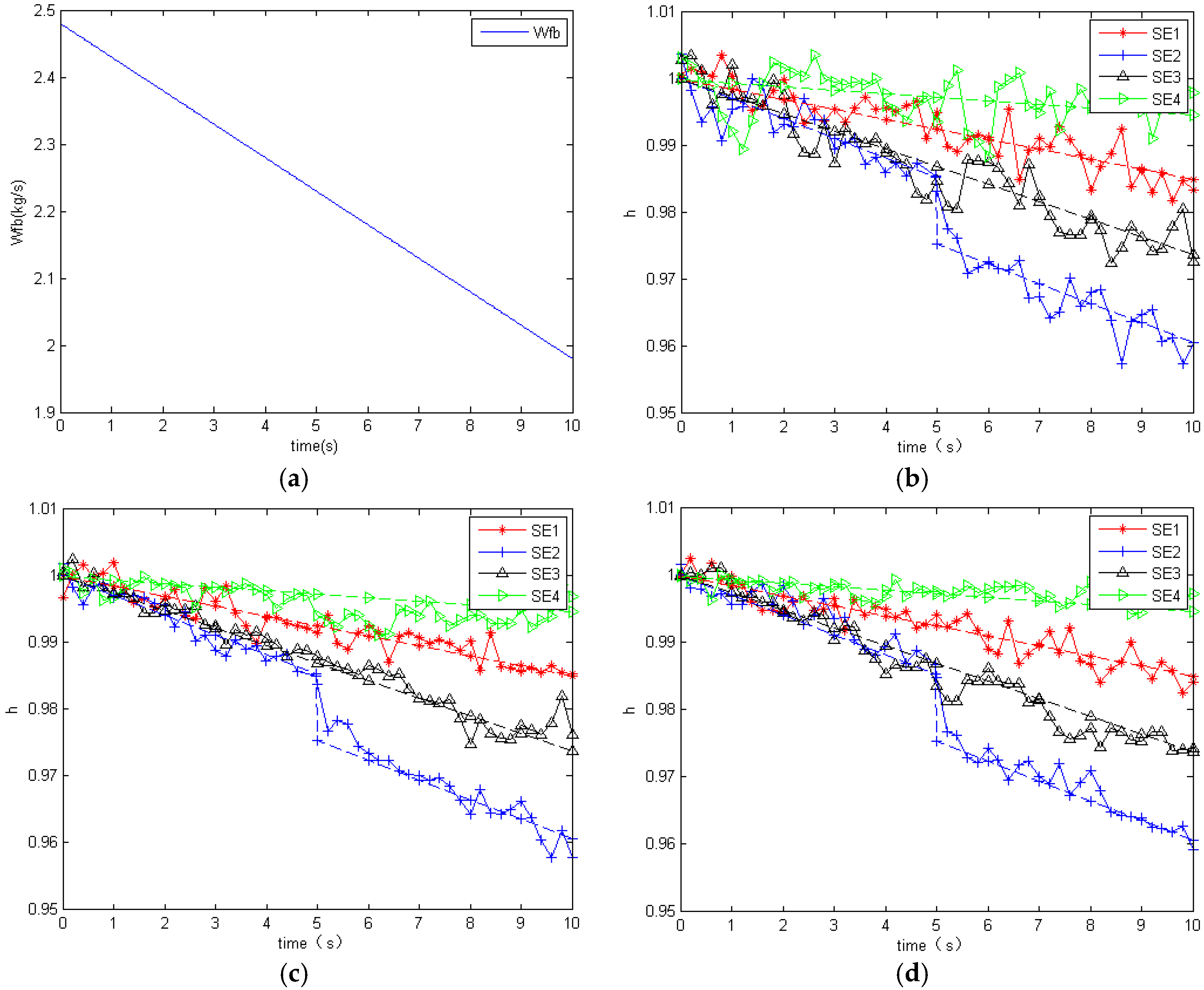
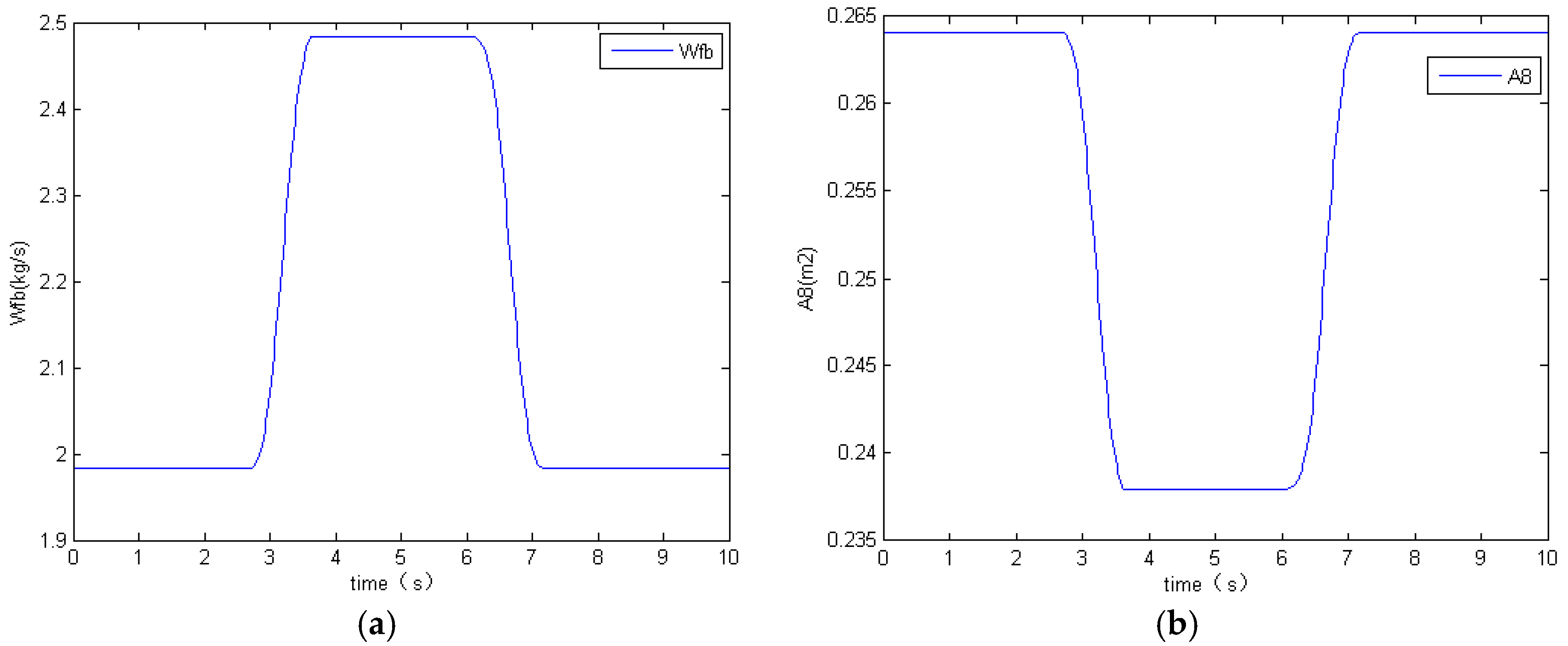
4.2. Abrupt Fault Diagnosis in Dynamic Operation

| Operation Condition | PF | F-PF | FA-PF |
|---|---|---|---|
| Ground | 0.0120 | 0.0077 | 0.0069 |
| High-altitude 1 | 0.0124 | 0.0076 | 0.0069 |
| High-altitude 2 | 0.0123 | 0.0079 | 0.0070 |
4.3. Performance Estimation with Uncertain Noise in Dynamic Operation

| σ | Uncertain Noise of Sensor P22 | ||||
| R0 | R1 | R2 | True Value | Tuning Value | |
| RMSE | 0.0121 | 0.0109 | 0.0108 | 0.0085 | 0.0088 |
| σ | Uncertain Noise of All Sensors | ||||
| R0 | 2R0 | 3R0 | True Value | Tuning Value | |
| RMSE | 0.0165 | 0.0116 | 0.0169 | 0.0095 | 0.0096 |
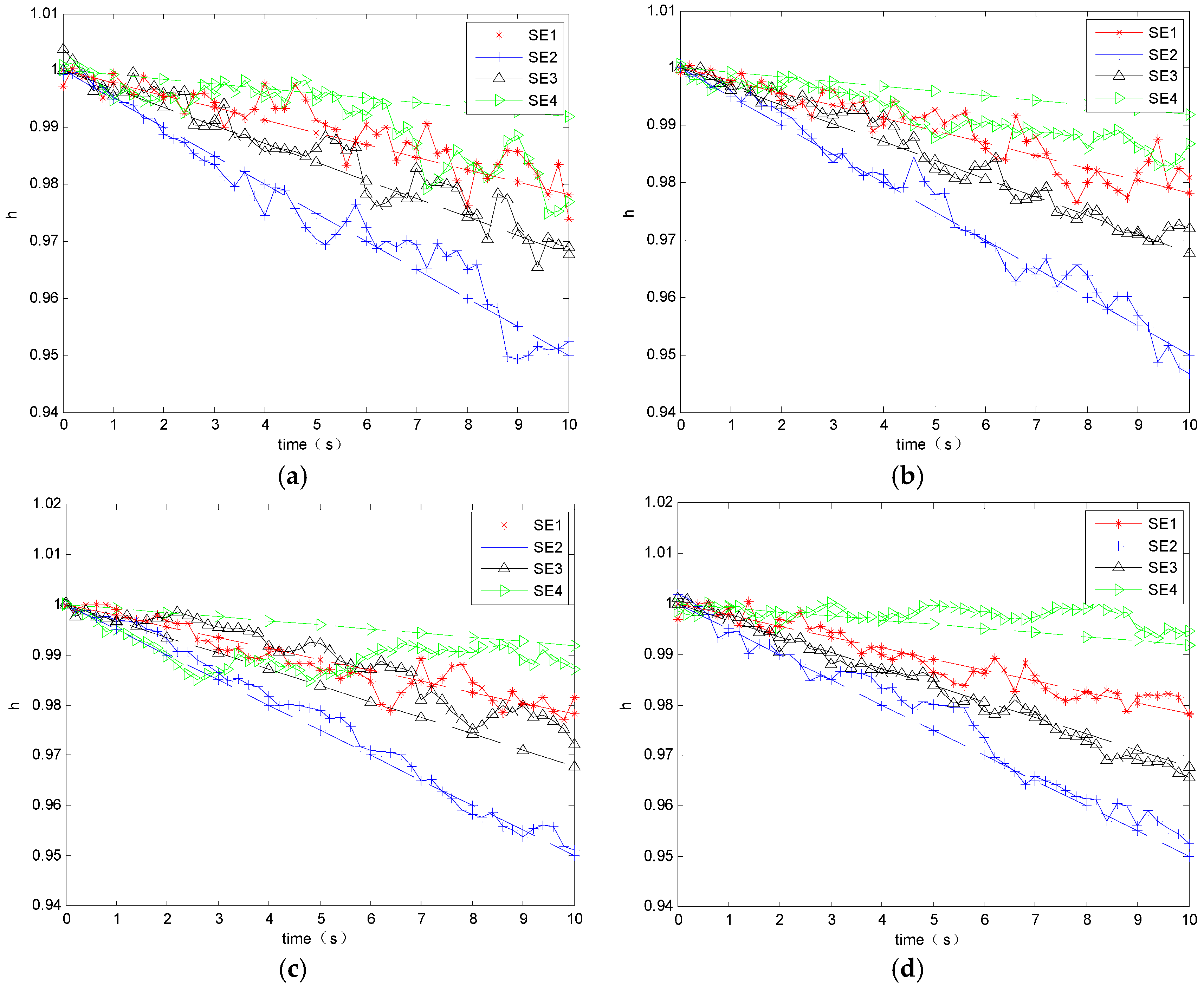
4.4. Engine Health Monitoring Test
| Fault Modes | RMSE | RMSD | ||||||
|---|---|---|---|---|---|---|---|---|
| PF | F-PF | FC-PF | FA-PF | PF | F-PF | FC-PF | FA-PF | |
| Case 1 | 0.0140 | 0.0101 | 0.0084 | 0.0061 | 0.0123 | 0.0083 | 0.0075 | 0.0050 |
| Case 2 | 0.0138 | 0.0095 | 0.0078 | 0.0055 | 0.0119 | 0.0079 | 0.0069 | 0.0043 |
| Case 3 | 0.0134 | 0.0100 | 0.0089 | 0.0058 | 0.0117 | 0.0069 | 0.0079 | 0.0050 |
| Case 4 | 0.0144 | 0.0106 | 0.0094 | 0.0065 | 0.0132 | 0.0077 | 0.0079 | 0.0052 |
5. Conclusions
Acknowledgments
Author Contributions
Conflicts of Interest
References
- Volponi, A. Gas turbine engine health management: Past, present, and future trends. J. Eng. Gas Turbines Power 2014, 136. [Google Scholar] [CrossRef]
- Rodger, J.A. Toward reducing failure risk in an integrated vehicle health maintenance system: A fuzzy multi-sensor data fusion Kalman filter approach for IVHMS. Expert Syst. Appl. 2012, 39, 9821–9836. [Google Scholar] [CrossRef]
- Borguet, S.; Léonard, O. Comparison of adaptive filters for gas turbine performance monitoring. J. Comput. Appl. Math. 2010, 234, 2202–2212. [Google Scholar] [CrossRef]
- Li, Y.G.; Korakianitis, T. Nonlinear weighted-least-squares estimation approach for gas-turbine diagnostic applications. J. Propuls. Power 2011, 27, 337–345. [Google Scholar] [CrossRef]
- Joly, R.B.; Ogaji, S.O.T.; Singh, R.; Probert, S.D. Gas-turbine diagnostics using artificial neural-networks for a high bypass ratio military turbofan engine. Appl. Energy 2004, 78, 397–418. [Google Scholar] [CrossRef] [Green Version]
- Vanini, Z.N.S.; Khorasani, K.; Meskin, N. Fault detection and isolation of a dual spool gas turbine engine using dynamic neural networks and multiple model approach. Inf. Sci. 2014, 259, 234–251. [Google Scholar] [CrossRef]
- Eustace, R.W. A real-world application of fuzzy logic and influence coefficients for gas turbine performance diagnostics. J. Eng. Gas Turbines Power 2008, 130. [Google Scholar] [CrossRef]
- Simon, D. A comparison of filtering approaches for aircraft engine health estimation. Aerosp. Sci. Technol. 2008, 12, 276–284. [Google Scholar] [CrossRef]
- Sun, J.G.; Vasilyev, V.; Ilyasov, B. Advanced Multivariable Control Systems of Aeroengines; Beihang Press: Beijing, China, 2005; pp. 60–83. [Google Scholar]
- Lu, F.; Chen, Y.; Huang, J.Q.; Zhang, D.D. An integrated nonlinear model-based approach to gas turbine engine sensor fault diagnostics. J. Aerosp. Eng. 2014, 228, 2007–2021. [Google Scholar] [CrossRef]
- Volponi, A. Enhanced Self Tuning On-Board Real-Time Model (eSTORM) for Aircraft Engine Performance Health Tracking; Technical Report for National Aeronautics and Space Administration: Cleveland, OH, USA, 2008. [Google Scholar]
- Armstrong, J.B.; Simon, D.L. Implementation of an Integrated On-Board Aircraft Engine Diagnostic Architecture; Technical Report for National Aeronautics and Space Administration: Cleveland, OH, USA, 2012. [Google Scholar]
- Simon, D. Kalman filtering with state constraints: A survey of linear and nonlinear algorithms. IET Control Theory Appl. 2010, 4, 1303–1318. [Google Scholar] [CrossRef]
- Lu, F.; Huang, J.Q.; Lv, Y.Q. Gas path health monitoring for a turbofan engine based on a nonlinear filtering approach. Energies 2013, 6, 492–513. [Google Scholar] [CrossRef]
- Gordon, N.; Salmond, D.; Smith, A. Novel Approach to Nonlinear/Non-Gaussian Bayesian State Estimation. IEE Proc. F Radar Signal Process. 1993, 140, 107–113. [Google Scholar] [CrossRef]
- Climente-Alarcon, V.; Antonino-Daviu, J.A.; Haavisto, A.; Arkkio, A. Particle filter-based estimation of instantaneous frequency for the diagnosis of electrical asymmetries in induction machines. IEEE Trans. Instrum. Meas. 2014, 63, 2454–2463. [Google Scholar] [CrossRef]
- Zhao, B.; Skjetne, R.; Blanke, M.; Dukan, F. Particle filter for fault diagnosis and robust navigation of underwater robot. IEEE Trans. Control Syst. Technol. 2014, 22, 2399–2407. [Google Scholar] [CrossRef]
- Tao, G.L.; Deng, Z.L. Self-tuning fusion Kalman filter for multisensor single-channel ARMA signals with coloured noises. IMA J. Math. Control Inf. 2015, 32, 55–74. [Google Scholar] [CrossRef]
- Zhu, H.Y.; Zhai, Q.Z.; Yu, M.W.; Han, C.Z. Estimation fusion algorithms in the presence of partially known cross-correlation of local estimation errors. Inf. Fusion 2014, 18, 187–196. [Google Scholar] [CrossRef]
- Seifzadeh, S.; Khaleghi, B.; Karray, F. Distributed soft-data-constrained multi-model particle filter. IEEE Trans. Cybern. 2015, 45, 384–394. [Google Scholar] [CrossRef] [PubMed]
- Zajac, M. Online fault detection of a mobile robot with a parallelized particle filter. Neurocomputing 2014, 126, 151–165. [Google Scholar] [CrossRef]
- Li, T.C.; Sun, S.D.; Sattar, T.P. Fight sample degeneracy and impoverishment in particle filters: A review of intelligent approaches. Expert Syst. Appl. 2014, 41, 3944–3954. [Google Scholar] [CrossRef]
- Simon, D. Constrained Kalman Filtering via Density Function Truncation for Turbofan Engine Health Estimation; Technical Report for National Aeronautics and Space Administration: Cleveland, OH, USA, 2006. [Google Scholar]
- Boulkroune, B.; Darouach, M.; Zasadzinski, M. Moving horizon state estimation for linear discrete-time singular systems. IET Control Theory Appl. 2010, 4, 339–350. [Google Scholar] [CrossRef]
- Yadav, S.K.; Sinha, R.; Bora, P.K. Electrocardiogram signal denoising using non-local wavelet transform domain filtering. IET Signal Process. 2015, 9, 88–96. [Google Scholar] [CrossRef]
- Kyriazis, A.; Mathioudakis, K. Enhance of fault localization using probabilistic fusion with gas path analysis algorithms. J. Eng. Gas Turbines Power 2009, 131. [Google Scholar] [CrossRef]
- Kaltungo, A.Y.; Sinha, J.K.; Elbhbah, K. An improved data fusion technique for faults diagnosis in rotating machines. Measurement 2014, 58, 27–32. [Google Scholar] [CrossRef]
- Curnock, B. Obidicote Project—Work Package 4: Steady-State Test Cases; Rolls-Royce PLC: Manchester, UK, 2000. [Google Scholar]
- Hultgren, L.S.; Miles, J.H. Noise-Source Separation Using Internal and Far-Field Sensors for a Full-Scale Turbofan Engine. In Proceedings of the 15th AIAA/CEAS Aeroacoustics Conference (30th AIAA Aeroacoustics Conference) Cosponsored by AIAA and CEAS, Miami, FL, USA, 11–13 May 2009.
© 2015 by the authors; licensee MDPI, Basel, Switzerland. This article is an open access article distributed under the terms and conditions of the Creative Commons by Attribution (CC-BY) license (http://creativecommons.org/licenses/by/4.0/).
Share and Cite
Lu, F.; Wang, Y.; Huang, J.; Huang, Y. Gas Turbine Transient Performance Tracking Using Data Fusion Based on an Adaptive Particle Filter. Energies 2015, 8, 13911-13927. https://doi.org/10.3390/en81212403
Lu F, Wang Y, Huang J, Huang Y. Gas Turbine Transient Performance Tracking Using Data Fusion Based on an Adaptive Particle Filter. Energies. 2015; 8(12):13911-13927. https://doi.org/10.3390/en81212403
Chicago/Turabian StyleLu, Feng, Yafan Wang, Jinquan Huang, and Yihuan Huang. 2015. "Gas Turbine Transient Performance Tracking Using Data Fusion Based on an Adaptive Particle Filter" Energies 8, no. 12: 13911-13927. https://doi.org/10.3390/en81212403