Unit Commitment Model Considering Flexible Scheduling of Demand Response for High Wind Integration

Abstract

In this paper, a two-stage stochastic unit commitment (UC) model considering flexible scheduling of demand response (DR) is proposed. In the proposed UC model, the DR resources can be scheduled: (1) in the first stage, as resources on a day-ahead basis to integrate the predicted wind fluctuation with lower uncertainty; (2) in the second stage, as resources on an intra-day basis to compensate for the deviation among multiple wind power scenarios considering the coupling relationship of DR on available time and capacity. Simulation results on the Pennsylvania-New Jersey-Maryland (PJM) 5-bus system and IEEE 118-bus system indicate that the proposed model can maximize the DR value with lower cost. Moreover, different types of DR resources may vary in the contract costs (capacity costs), the responsive costs (energy costs), the time of advance notice, and the minimum on-site hours. The responsive cost is considered as the most important factor affecting DR scheduling. In addition, the first-stage DR is dispatched more frequently when transmission constraints congestion occurs.

1. Introduction

The expansion of variable wind power imposes challenges on the system operation, and these challenges mainly stem from unpredictability, the steep ramping requirement [1], intra-hour variability, and over-generation in the middle of the night [2,3]. Advanced scheduling strategies and much more flexible resources are required to accommodate the growing variability and uncertainty.

Shortages of generator ramp capability are anticipated to worsen in the future because of the growth of wind generation and, in some cases, the retirement of flexible thermal capacity. Demand Response (DR), which can be flexibly deployed to follow wind power generation, is investigated as an effective way to address the above challenges [4]. Generally, DR can provide load shifting/reduction and various ancillary services, such as regulation, spinning reserve, non-spinning reserve, and ramping for integrating renewable energy [5]. Many studies have demonstrated the effectiveness of DR for achieving lower operational cost [6,7,8], higher wind power utilization [9], and lower carbon emission [10,11].

Previous works mitigated wind power uncertainty by combining stochastic unit commitment (SUC) and DR. In the existing literatures on DR in combination with stochastic programming, DR resources are generally regarded as flexible resources to meet the needs of multiple scenarios to participate in the second stage decision, that is, they are configured as an intra-day basis (in the second-stage) to participate in system scheduling. Reference [12] illustrated that the issue of wind power forecasting errors can be partly solved by flexible demand based on an SUC model considering price-based DR. However, the transmission constraint is not included in [12], and price-based DR is only scheduled in the second stage. In [13], the impacts of DR and stochastic optimization are examined to demonstrate that both DR and stochastic programming can be used to mitigate wind power uncertainty, but DR was significantly more effective than stochastic programming for reducing the costs caused by wind power uncertainty. Reference [13] is concerned with the impacts of stochastic programming and demand response on wind integration and preliminary indicates the impacts of using demand response and stochastic optimization. Moreover, the DR characteristics are described relatively simple. In [14], a SUC model is proposed considering renewable resources and DR. In the aforementioned papers, DR was used to provide reserves for addressing uncertainties and was scheduled only in the second stage to provide reserves. In [15], a two-stage stochastic model is presented to schedule energy and reserves from both generating units and responsive loads with high wind penetration. In [15], incentive-based DR participates in the energy market and reserves market, but the coupling relationship on time and capacity is not highlighted and the difference of flexibility between first-stage DR and second-stage DR is not considered. Besides, DR operating cost in the first-stage (a day-ahead basis) is the same with that in the second-stage (an intra-day basis). The work in [15] demonstrated that DR could be used to address the challenge of wind power uncertainty as well as reduce operational costs and emissions. The model in [16] is linear programming, i.e., deterministic programming. In addition, it focuses on the coupling of photovoltaic, battery storage and conventional sources rather than DR resources. In [17], DR is modeled as a flexible generator that can start and shut down at any time. Only the capacity coupling characteristics of DR are considered, that is, the scheduled DR reserves (less than scheduled reserves) are second-stage decisions. In the existing published literatures, the DR resources are all in the second stage of scheduling as resources on an intra-day basis. Although in this way it can take the advantage that DR flexibly dispatched on an intra-day basis according to the system operating requirement, there are still three disadvantages: (1) DR usually requires a high level of incentive mechanism; (2) DR all on an intra-day basis will increase the difficulties of scheduling; (3) in the models available in the literature, the DR resources are restricted by time scale, and the coupling relationship on time and capacity is ignored. All of these shortcomings above mentioned limit the flexibility advantages of DR to some extent.

DR commitment as an alternative flexible resource to address the challenges of high wind power integration receives increasing attentions. However, current research on DR scheduling mainly focuses on the scheduling of different types of DR programs in a separated timescale, ignoring the tight coupling characteristics of specific DR resources on the available time frame and capacity. This may prevent distributed flexible DR resources from facilitating system balance and renewable energy integration on different time scales. The amount of flexible resources from conventional units is fixed due to the initial design. Those resources may be reduced because the expansion of wind power results in retirement of thermal units. These factors lead to some interesting questions:

(1)

What is the effect of DR on the system operation flexibility of a power grid with large-scale renewable energy integration?

(2)

How can the effectiveness be maximized at minimum cost using the flexible scheduling strategies of DR considering the coupling characteristics of centralized, controlled DR resources?

(3)

Which characteristic of DR will affect the flexible schedule performance and what is the turnkey? What are the impacts of the transmission constraints?

In this paper, we examine these topics with a SUC model that incorporates the flexible scheduling of DR. Compared with previous works, the main contributions of this paper can be summarized as follows: (1) this paper explores a new model to schedule flexible DR resources that can achieve the maximal DR benefits with the minimal cost, considering the cost advantage of DR on a day-ahead basis (first stage) and the flexibility advantage of DR on an intra-day basis (second stage). The DR modeling way above mentioned is very beneficial for high wind power penetration; (2) demand response features are fully modeled. DR operating costs on a day-ahead basis is less than that on an intra-day basis, because the advance notice time in the first stage is longer than that in the second stage; (3) flexible scheduling and allocation of dispatchable DR programs based on the tight coupling characteristic of specific DR resources on the available time and capacity is proposed. In the case study, the effect of flexible scheduling of DR is illustrated.

The rest of this paper is organized as follows: Section 2 summarizes the stochastic programming with flexible scheduling of DR. Section 3 presents the mathematical formulation. Numerical examples are then provided in Section 4 and Section 5 concludes the paper.

2. Problem Definition

This paper focuses on flexibly scheduling DR resources in a two-stage stochastic programming process to achieve efficient wind power integration. The uncertainty of wind power output is considered in this paper, and the uncertainty is modeled with various wind power scenarios. All conventional units are assumed to be coal-fired plants for better illustration of the wind power and DR (in China, thermal power generators account for 80% of overall power generation, therefore in this paper, all the conventional units are referred to as coal-fired plants).

2.1. Stochastic Unit Commitment

The previous studies in [12,13,14,15] adopted a two-stage stochastic model considering co-optimization of DR and conventional units to meet the fluctuating net load (load forecasted minus output of renewable energy) of different scenarios. They modeled DR resources on either a day-ahead basis or an intra-day basis. Some papers take DR reserve variables as first-stage decisions, whereas in some papers, these variables are treated in the second-stage, such as [18]. However, the DR resources can be flexibly scheduled as resources on both a day-ahead and an intra-day basis according to the requirement of system operation under the premise of certain constraints. For instance, conventional slow units, as well as part of the DR programs, such as price-based programs, will be committed and dispatched in the day-ahead time scale. In addition, quick units and some DR programs (e.g., direct load control, interruptible load) can be dispatched as intra-day resources after the wind power scenario has been revealed. However, one DR program may affect the performance of another DR program in practice. For instance, a DR aggregator can call a peak-time-price event [19] on a day-ahead basis if a power shortage during the peak time is forecasted for the next day. Meanwhile, the aggregator may dispatch direct load control (DLC) one or two hours ahead of the shortage event during the operation day. This may be affected by the peak-time-price program if it was activated one day ahead. Therefore, one consumer’s DR performance or potential may change if he/she participates in a day-ahead, price-based program because his/her initial load baseline is changed. The sequence of decisions in the proposed model is shown in Figure 1.

In the stochastic programming, the first-stage variables represent commitments made before it is known which scenario will occur, DR resources in the first stage (on a day-ahead basis) usually result from consumers' production plan adjustment. However, the second-stage variables are scenario-specific and are chosen after the scenario is known. DR resources in the second stage (on an intra-day basis) are often activated by turning devices on/off, which causes much greater losses compared with production plan adjustment. In our model, DR-related variables can be either first-stage or second-stage. For instance, DR binary on/off variables $v_{d,t}$, DR capacity variables $\text{max}{D}_d$ and DR resources of a day-ahead notice are first-stage and are decided on a day-ahead basis. However, the variables of the load not served $cur{t}_{i,t,s}^{load}$ and wind curtailment $cur{t}_{i,t,s}^{wind}$ are scenario-specific, which are chosen on an intra-day basis. This “split” is conducive to better illustrate the effect of DR in the proposed model.

Figure 1. Sequence of decisions in the stochastic unit commitment (SUC) problem with flexibly scheduled demand response (DR).

Figure 1. Sequence of decisions in the stochastic unit commitment (SUC) problem with flexibly scheduled demand response (DR).

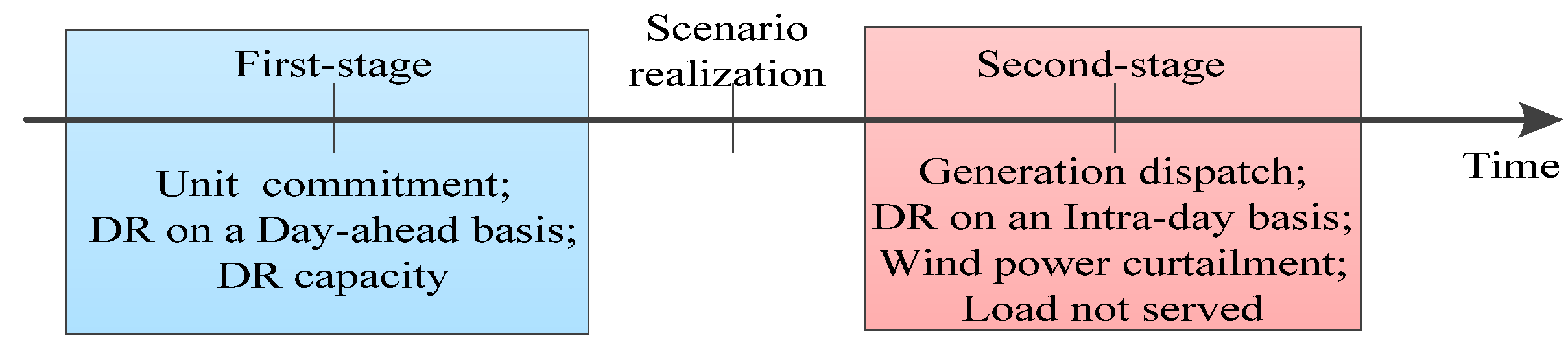
2.2. Demand Flexibility

DR programs can be classified into two major categories: price-based and incentive-based [20]. The former refers to an entirely voluntary response to prices by users, whereas the latter involves load change motivated by contract-based payments. However, price-based DR is identified as non-dispatchable. Incentive-based DR can be regarded as dispatchable because there are penalties for customers who are enrolled but do not respond as required. In other words, incentive-based DR has a relatively reliable and effective response performance.

Because this paper is mainly concerned with flexible scheduling and allocation of dispatchable DR programs based on the coupling relationship of available time and capacity, the optimal incentive level to obtain a reliable response will not be discussed. This paper assumes that given the incentive levels, DR providers will reliably increase/decrease demand to meet the balance requirements. Generally speaking, the rescheduling costs of consumers are inversely proportional to the time of the advanced notice. Shorter advanced notice time causes a greater impact on operational processes, which may result in less consumer surplus. For instance, DR resources on a day-ahead basis usually result from consumers' production plan adjustment. However, DR resources on an intra-day basis are often activated by turning devices on/off, which will cause much more losses if compared with production plan adjustment. Accordingly, the DR on a day-ahead basis has lower incentive payments but greater limitations on implementation, whereas DR on an intra-day basis requires a much higher incentive level but has fewer constraints. In other words, day-ahead resources are cheaper but inflexible, whereas intra-day resources are expensive but flexible.

Furthermore, some DR could be scheduled both: (1) in the first stage as resources on a day-ahead basis to integrate the predicted wind power with lower uncertainty; (2) in the second stage as resources on an intra-day basis to compensate for the deviation among multiple wind power scenarios. In more practical terms, a certain DR could be equivalent to both slow generators and fast ones to adapt to the requirement of wind power integration.

DR-related constraints considering two-stage coupling in the proposed model are shown as follows:

(1)

Constraints for the first stage:

• minimum onsite hours called once;
• maximum times called during a defined period;
• minimum/maximum responsive capacity.

(2)

Constraints for the second stage:

• maximum responsive capacity.

(3)

Coupled constraints for both stages:

• maximum capacity of DR of the sum of two stages.

Additionally, a responsive load bid consists of a capacity component and an energy component in each stage. A detailed model will be presented in the following section.

3. Problem Formulation

DR aggregators are considered in this study as the unique resources vender because they have a perfect response performance due to the professionals in program implementation. In this section, the two-stage SUC model with flexible scheduling of DR is proposed. The first-stage decision consists of three parts: (1) UC of slow conventional units; (2) total available DR capacity for both stages, (3) demand response dispatch on a day-ahead basis. The second stage also includes three parts: (1) units output levels; (2) demand response dispatched on an intra-day basis; (3) wind and load curtailment.

3.1. Objective Function

$$\begin{array}{l}\text{Min\hspace{0.17em}}F={\displaystyle \sum _{s=1}^{N_s}{\displaystyle \sum _{t=1}^{N_T}{\mathrm{Pr}}_{s,t}}}[{\displaystyle \sum _{n=1}^{N_g}f({\text{p}}_{n,t,s})+}{\displaystyle \sum _{d=1}^{N_d}E{c}_{d2}^{+}\times d{2}_{d,t,s}^{+}}+{\displaystyle \sum _{d=1}^{N_d}E{c}_{d2}^{-}\times d{2}_{d,t,s}^{-}}+{\displaystyle \sum _{\omega =1}^{N_{\omega }}Pen{a}_{\omega }\times cur{t}_{i,t,s}^{wind}}+{\displaystyle \sum _{i=1}^{N_b}Pen{a}_l\times cur{t}_{i,t,s}^{load}}]\\ +{\displaystyle \sum _{t=1}^{N_T}{\displaystyle \sum _{n=1}^{N_g}s\_\cos t_{n,t}}}+{\displaystyle \sum _{d=1}^{N_d}C{c}_d\times \max D_d}+{\displaystyle \sum _{t=1}^{N_T}{\displaystyle \sum _{d=1}^{N_d}E{c}_{d1}^{+}\times d{1}_{d,t}^{+}}}+{\displaystyle \sum _{t=1}^{N_T}{\displaystyle \sum _{d=1}^{N_d}E{c}_{d1}^{-}\times d{1}_{d,t}^{-}}}\end{array}$$

(1)

The objective Equation (1) is used to minimize the total expected cost, which includes generation costs, start-up costs, DR costs, and wind power and load curtailment costs under all scenarios. DR costs include capacity costs and operating costs. The load not served $cur{t}_{i,t,s}^{load}$ is different from the demand level reduction $d{1}_{d,t}^{-}$ and $d{2}_{d,t,s}^{-}$ $cur{t}_{i,t,s}^{load}$ only occurs when the flexibility of the system is binding. In other words, $cur{t}_{i,t,s}^{load}$ is a slack variable to ensure that the proposed model has a solution, but the associated penalty should be very high if $cur{t}_{i,t,s}^{load}$ actually occurs. In Equation (1), unit commitment decision u_n,t, DR capacity maxD_d and demand level growth/reduction on an day-ahead basis $d{1}_{d,t}^{+}$ and $d{1}_{d,t}^{-}$ are first-stage variables. In addition, the unit generation $p_{n,t,s}$, demand level growth/reduction on an intra-day basis $d{2}_{d,t,s}^{+}$ and $d{2}_{d,t,s}^{-}$, wind power curtailment $cur{t}_{i,t,s}^{wind}$ and load not served $cur{t}_{i,t,s}^{load}$ are second-stage decisions, so they are scenario-specific and take probability into account. DR capacity $\text{max}{D}_d$ is a first-stage decision variable representing the upper bound of the total load growth/reduction of the two stages.

3.2. Constraints

3.2.1. Power Balance

$${\displaystyle \sum _{n\in G_i}{p}_{n,t,s}}+win{d}_{i,t,s}-cur{t}_{i,t,s}^{wind}-{\displaystyle \sum _{j\in I,i\ne j}{B}_{ij}({\theta }_{i,t,s}-{\theta }_{j,t,s})}=Loa{d}_{i,t}+{\displaystyle \sum _{d\in D_i}(d{1}_{d,t}^{+}-d{1}_{d,t}^{-}+d{2}_{d,t,s}^{+}-d{2}_{d,t,s}^{-}})-cur{t}_{i,t,s}^{load}\forall i,j\in N_b,t\in N_T$$

(2)

Equation (2) ensures system power balance for all times in each scenario.

3.2.2. Network Constraint

$$-TR{C}_{ij}\le B_{ij}({\theta }_{i,t,s}-{\theta }_{j,t,s})\le TR{C}_{ij}\forall i,j\in N_b,t\in N_T,s\in N_s$$

(3)

Constraint Equation (3) limits the line flow from exceeding the capacity of transmission line between nodes i and j.

3.2.3. Constraints for Conventional Units

$$u_{n,t}{P}_n^{\min }\le p_{n,t,s}\le u_{n,t}{P}_n^{\max }\begin{array}{cc}& \forall n\in N_g,t\in N_T,s\in N_s\end{array}$$

(4)

$$\{\begin{array}{l}{p}_{n,t,bs}-p_{n,t-1,bs}\le R_n^{up}\\ p_{n,t-1,bs}-p_{n,t,bs}\le R_n^{down}\end{array}\forall n\in N_g,t\in N_T$$

(5)

$$\left|p_{n,t,s}-p_{n,t,bs}\right|\le {\mathsf{\Delta }}_n\forall n\in N_g,t\in N_T,s\in N_s$$

(6)

$$\{\begin{array}{l}(u_{n,t-1}-u_{n,t})+(u_{n,t+\tau }-u_{n,t+\tau -1})\le 1\\ \forall \tau \in [1,\cdots ,M{D}_n-1]\\ (u_{n,t}-u_{n,t-1})+(u_{n,t+\tau -1}-u_{n,t+\tau })\le 1\\ \forall \tau \in [1,\cdots ,M{U}_n-1]\end{array}\forall n\in N_g,t\in N_T$$

(7)

$$s\_\cos t_{n,t}\ge S{c}_n*(u_{n,t}-u_{n,t-1})\forall n\in N_g,t\in N_T$$

(8)

$$s\_\cos t_{n,t}\ge 0\forall n\in N_g,t\in N_T$$

(9)

Generation output levels are limited by the minimum and maximum output levels, as shown in Equation (4). Constraint Equation (5) ensures that the generation output fluctuation in two consecutive periods under the base scenario (bs) is within the ramp rates, whereas Equation (6) guarantees the secure and economic transfer of system operation from the base scenario (bs in Equation (5)) to all scenarios at each hour [21,22]. Constraint Equation (7) is used to meet the minimum down/up-time requirement of unit n, and Equations (8) and (9) ensure that the start-up costs are only incurred when a unit is turned on.

3.2.4. Constraints for DR

$$\{\begin{array}{l}{v}_{d,t}D{R}_d^{\min }\le d{1}_{d,t}^{+}\le \max D_d\\ v_{d,t}D{R}_d^{\min }\le d{1}_{d,t}^{-}\le \max D_d\end{array}\forall d\in N_d,t\in N_T$$

(10)

$$\begin{array}{l}(v_{d,t}-v_{d,t-1})+(v_{d,t+\tau -1}-v_{d,t+\tau })\le 1\\ \forall d\in N_d,t\in N_T\forall \tau \in [1,\cdots ,MD{T}_d-1]\end{array}$$

(11)

$$\{\begin{array}{l}0\le d{1}_{d,t}^{+}+d{2}_{d,t,s}^{+}\le \max D_d\\ 0\le d{1}_{d,t}^{-}+d{2}_{d,t,s}^{-}\le \max D_d\end{array}\forall d\in N_d,t\in N_T,s\in N_s$$

(12)

$$0\le \max D_d\le {\nu }_{d,t}D{R}_d^{\max }\forall d\in N_d,t\in N_T$$

(13)

$${\displaystyle \sum _{t=1}^{N_T}[(d{1}_{d,t}^{+}+d{2}_{d,t,s}^{+})-(d{1}_{d,t}^{-}+d{2}_{d,t,s}^{-})}]=0\begin{array}{cc}& \forall d\in N_d,t\in N_T,s\in N_s\end{array}$$

(14)

Constraints (10) and (11) are associated with the DR on a day-ahead basis, i.e., the first-stage DR, and they are scenario-independent and fixed for all scenarios. Constraint (10) restricts the responsive load of the first stage to within the DR capacity, whereas Equation (11) indicates the minimum on-site hours of DR. Constraint (11) is necessary because DR resources on a day-ahead basis usually result from consumers’ production plan adjustment, proceeding for several hours. Constraint (12) is the coupling DR capacity relationship between the two stages. In the first stage, the minimum/maximum responsive capacity constraint is considered. In the second stage, there is maximum responsive capacity constraint. Moreover, maximum capacity of DR of the sum of two stages is also included, which is the coupled constraints for both stages. Constraint (13) ensures that DR capacity is no more than the max responsive load. Equation (14) (if a rebound effect is included, the rebound load level after DR event can be modeled as a weighted sum of shedding load values for t − 1, t − 2 and t − 3, as illustrated in [23]. In our future research works, we will consider the rebounding effect in a deterministic model.) ensures the demand level reduction is recovered in another period, which is regarded as perfect load shifting [24]. In this paper, we assumed perfect load shifting, i.e., no rebound effect is considered (the proposed model is focused on flexible scheduling and allocation of dispatchable DR programs based on the coupling relationship of available time and capacity; the rebound effect is not considered), because the simplified assumption better explains the effect of the flexible scheduling of DR.

3.2.5. Non-Negativity

$$\{\begin{array}{l}{p}_{n,t,s},cur{t}_{i,t,s}^{wind},cur{t}_{i,t,s}^{load}\ge 0\\ d{1}_{d,t}^{+},d{1}_{d,t}^{-},d{2}_{d,t,s}^{+},d{2}_{d,t,s}^{-},\max D_d\ge 0\end{array}$$

(15)

4. Case Study

A modified PJM 5-bus system [25] and the IEEE 118-bus system [26] are adopted in this case study. The PJM 5-bus system is small, but the results are easier to understand. Therefore, more detailed analysis is discussed in the case study of the PJM 5-bus system. Firstly, the case without a transmission constraint is explored to verify the effect of the proposed model and to explore the key factors associated with flexible scheduling of DR. Then, the effect of the transmission constraint on flexible scheduling of DR is analyzed. The IEEE 118-bus system is used to demonstrate the applicability of the proposed model to larger systems. The case studies are based on CPLEX 12.1 and YALMIP under MATLAB software (The MathWorks, Inc., Natick, MA, USA.).

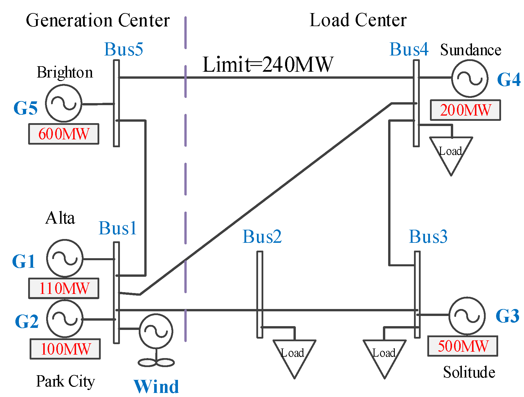
4.1. PJM5-Bus System

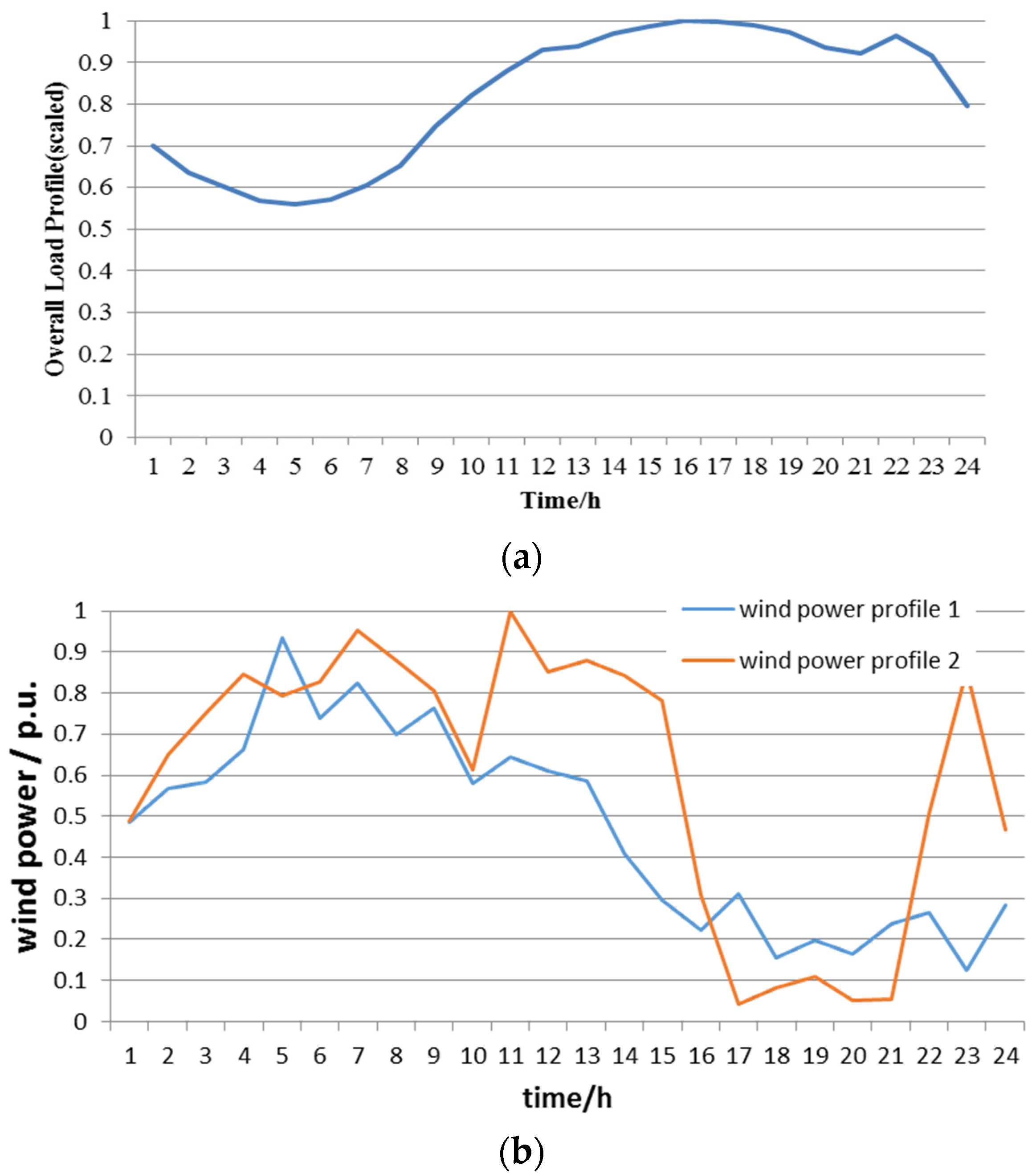
4.1.1. Data Assumption

Figure 2 shows the topology of the modified PJM 5-bus system. The wind farm is added at Bus1, and the DR resources are located at Bus 4.The load benchmark without DR [27] is shown in Figure 3, and the nodal load is 3/10, 3/10 and 4/10 of the aggregated load. The assumed wind power forecast scenarios (in fact, the number of wind power scenarios predicted was far more than three, and actually 2000. Most of them were then cut and concentrated to three scenarios. Since the aim of this paper is not to explore scenario reduction techniques but rather to discuss a stochastic unit commitment model considering direct load control scheduling, the steps of the wind power scenarios generation and wind power scenarios cut were omitted. Detailed steps can be found in [28,29,30,31]) are shown in Figure 4. The scenario production and reduction is similar to [32]. The main parameters of units and DR providers can be obtained from Table 1 and Table 2, respectively.

Figure 2. Modified PJM 5-bus system.

Figure 2. Modified PJM 5-bus system.

Two kinds of wind power profiles, shown in Figure 3b are considered [33,34,35]. The wind power profiles were created using data from the National Renewable Energy Laboratory (NREL) Western Wind Integration Study based on two Southern California locations [36]. Combining the two kinds of 24 h original wind output profiles with the peak-normalized aggregate load benchmark in Figure 3, 2000 wind power forecast scenarios were generated according to the proposed wind power forecasting method. The prediction error of the output power of the wind farm was subject to the normal distribution, the mean value was 0.028, and the variance was 0.046. After that, the scenario reduction was carried out, and the number of the final scenarios of two wind power output profiles is 3 and 5 respectively [37,38,39], as shown in Figure 4 and Figure 7.

Figure 3. (a) Peak-normalized aggregate load benchmark; (b) Two kinds of peak-normalized wind power profiles respectively for three scenarios and five scenarios.

Figure 3. (a) Peak-normalized aggregate load benchmark; (b) Two kinds of peak-normalized wind power profiles respectively for three scenarios and five scenarios.

Figure 4. Peak-normalized wind power scenarios.

Figure 4. Peak-normalized wind power scenarios.

Table 1. Unit characteristics.

Unit	$P_n^{\min }$ (MW)	$P_n^{\max }$ (MW)	Incremental Cost ($/MWh)	Scn ($)	MDn/ MUn (h)	$R_n^{up}$/$R_n^{down}$ (MW/min)
G1	22	110	14	450	6/6	0.45
G2	20	100	15	900	6/6	0.42
G3	100	500	30	300	4/4	2
G4	60	200	40	150	1/1	0.8
G5	120	600	20	1200	6/6	2.5

Table 1. Unit characteristics.

Unit	$P_n^{\min }$ (MW)	$P_n^{\max }$ (MW)	Incremental Cost ($/MWh)	Scn ($)	MDn/ MUn (h)	$R_n^{up}$/$R_n^{down}$ (MW/min)
G1	22	110	14	450	6/6	0.45
G2	20	100	15	900	6/6	0.42
G3	100	500	30	300	4/4	2
G4	60	200	40	150	1/1	0.8
G5	120	600	20	1200	6/6	2.5

Table 2. DR Aggregator characteristics.

DR Aggregators	$D{R}_d^{\max }$ (MW)	$D{R}_d^{\min }$ (MW)	${\mathit{MDT}}_d$ (h)	$E{c}_{d1}^{\pm }$/$E{c}_{d2}^{\pm }$ ($/MWh)	$C{c}_d$ ($/MW)
1	35	3.5	4	8/20	15
2	25	2.5	4	6/25	15
3	25	2.5	8	5/16	15
4	35	3.5	8	2/23	15
5	20	2	1	10/15	15

Table 2. DR Aggregator characteristics.

DR Aggregators	$D{R}_d^{\max }$ (MW)	$D{R}_d^{\min }$ (MW)	${\mathit{MDT}}_d$ (h)	$E{c}_{d1}^{\pm }$/$E{c}_{d2}^{\pm }$ ($/MWh)	$C{c}_d$ ($/MW)
1	35	3.5	4	8/20	15
2	25	2.5	4	6/25	15
3	25	2.5	8	5/16	15
4	35	3.5	8	2/23	15
5	20	2	1	10/15	15

4.1.2. Results and Discussion

The results of several analyses are described here. In Subsection (1), we analyze the impact of flexible DR scheduling on cost without considering the transmission constraints. Then, in Subsection (2), we analyze the DR resources allocation among aggregators with different characteristics. Finally in Subsection (3), we explore the impact of transmission constraints.

(1) DR Scheduling Modes Impact on Costs

Four different DR scheduling modes: (1) ODR: without DR, (2) FDR: DR scheduled only in the first stage, (3) SDR: DR scheduled only in the second stage (the models available in the literature, in [13,19,33]) and (4) F&SDR: DR scheduled flexibly in two stages (the model proposed in this paper) are compared in Table 3 to illustrate the performance of the proposed model. The results indicate that DR is beneficial to system economy and wind power utilization as the total cost and wind power curtailment decrease when DR is scheduled in UCs. Moreover, DR scheduling modes have large effects on the results, as shown in Table 3. When DR is scheduled only in the first-stage, the generation cost decreases significantly, but the load not served increases slightly compared to that without DR because the flexibility of DR on a day-ahead basis (first-stage DR) is limited and does not allow for system balance of all scenarios without load curtailment. In contrast, when DR is scheduled only in the second stage, there is no wind and load curtailment because DR resources on an intra-day basis have enough flexibility to follow the system operation status and compensate for the deviation of various scenarios. However, DR scheduled capacity in this mode is less than the other two because the operating cost of DR on an intra-day basis is very high. In F&SDR (the last column of Table 3), there is a decrease in total costs relative to SDR because in Equation (1), $E{c}_{d1}^{\pm }$ (DR operating cost on a day-ahead basis; (2) $/MWh is less than $E{c}_{d2}^{\pm }$ (DR operating cost on an intra-day basis, 15 $/MWh), results in higher total cost because in SDR no first-stage DR resources are used. Additionally, the ability to maintain system balance (measured by wind curtailment costs and load not served costs) is enhanced relative to FDR. This result is expected because in the case of FDR, constraints (10) and (11) limit the available time to dispatch first-stage DR, resulting in much greater wind curtailment and load un-served. Accordingly, F&SDR attains optimal trade-offs between cost savings and the additional operating costs required to maintain system balance.

We consider other cases with more scenarios (such as five or ten scenarios) and a different wind power output profile, to assess if our results are artifacts of the exact system we considered. For brevity, we only briefly summarize the results. The results indicate that F&SDR always has higher flexibility and economic efficiency, as shown in Table 3.

Table 3. DR scheduling modes impact on cost when the wind power output is wind power profile 1: without transmission constraints.

Mode	ODR	FDR	SDR	F&SDR (Proposed Model)
Total Cost (103$)	Base (597.85)	−5.37	−60.05	−62.32
Generation Cost (103$)	Base (540.33)	−11.16	−7.25	−11.88
Start-up Cost (103$)	Base (0.30)	+0	+0	+0
Wind Curtailment Cost (103$)	Base (0.59)	−0.56	−0.59	−0.59
Load not served Cost (103$)	Base (56.63)	+0.56	−56.63	−56.63
DR Capacity Cost (103$)	Base (0)	+1.27	+0.62	+1.21
DR operating cost (103$)	Base (0)	+4.52	+3.80	+5.57

Table 3. DR scheduling modes impact on cost when the wind power output is wind power profile 1: without transmission constraints.

Mode	ODR	FDR	SDR	F&SDR (Proposed Model)
Total Cost (103$)	Base (597.85)	−5.37	−60.05	−62.32
Generation Cost (103$)	Base (540.33)	−11.16	−7.25	−11.88
Start-up Cost (103$)	Base (0.30)	+0	+0	+0
Wind Curtailment Cost (103$)	Base (0.59)	−0.56	−0.59	−0.59
Load not served Cost (103$)	Base (56.63)	+0.56	−56.63	−56.63
DR Capacity Cost (103$)	Base (0)	+1.27	+0.62	+1.21
DR operating cost (103$)	Base (0)	+4.52	+3.80	+5.57

In other studies, the cost of different modes with half capacity is analyzed. The cost is closer than the results in Table 3. The differences between ODR, FDR, SDR and F&SDR with respect to total cost is down to −3.35, −59.61, −60.82 (10³ $), respectively.

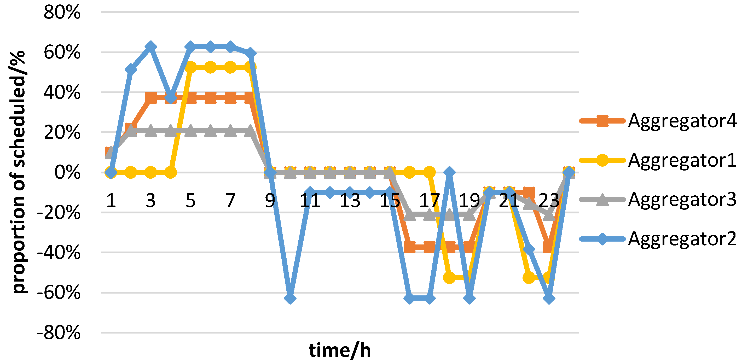
(2) DR Allocation among Aggregators with Different Characteristics: no Transmission Constraints

Firstly, the DR energy cost impact on resources dispatched in each stage is explored. The average proportion of DR scheduled in each stage for all aggregators is illustrated in Table 4. The second column of Table 4 represents the first-stage results; the last three columns show the values of three scenarios in the second stage. DR aggregator 4 is dispatched the most in the first stage, significantly more than DR aggregator 2, which has fewer minimum onsite hours MDT_d (4 h). This is reasonable because aggregator 4 has the lowest $E{c}_{d1}^{\pm }$ (DR operating cost on a day-ahead basis, 2 $/MWh, which is beneficial to decrease the total expected costs, object function Equation (1)). Similarly, DR aggregator 5, which has the lowest $E{c}_{d2}^{\pm }$ (DR operating cost on an intra-day basis, 15 $/MWh) provides a higher level of responsive load than others in the second stage. Combining Table 4 with Table 2, the average absolute proportion of DR scheduled for different DR aggregators is essentially consistent with their energy costs (first-stage/second-stage). Accordingly, the lower the cost is, the more the DR is dispatched when the transmission constraint is not considered.

Table 4. Average absolute proportion of DR scheduled in each stage for each aggregator (without transmission constraint).

DR Aggregators	First_s a	Second_s1 b	Second_s2 b	Second_s3 b
1	0%	0%	0%	7.13%
2	0%	0%	0%	0%
3	26.32%	11.48%	18.41%	17.59%
4	83.33%	0%	0%	0%
5	0%	16.96%	22.97%	26.31%

a: The average absolute proportion of DR scheduled in the first stage is calculated by ${\displaystyle \sum _{t=1}^{N_T}(d{1}_{d,t}^{+}+\left|d{1}_{d,t}^{-}\right|)}/N_T/D{R}_d^{\max }$; b: The average absolute proportion of DR scheduled in the second stage is calculated by ${\displaystyle \sum _{t=1}^{N_T}(d{2}_{d,t,s}^{+}+\left|d{2}_{d,t,s}^{-}\right|)}/N_T/D{R}_d^{\max }$.

Table 4. Average absolute proportion of DR scheduled in each stage for each aggregator (without transmission constraint).

DR Aggregators	First_s a	Second_s1 b	Second_s2 b	Second_s3 b
1	0%	0%	0%	7.13%
2	0%	0%	0%	0%
3	26.32%	11.48%	18.41%	17.59%
4	83.33%	0%	0%	0%
5	0%	16.96%	22.97%	26.31%

a: The average absolute proportion of DR scheduled in the first stage is calculated by ${\displaystyle \sum _{t=1}^{N_T}(d{1}_{d,t}^{+}+\left|d{1}_{d,t}^{-}\right|)}/N_T/D{R}_d^{\max }$; b: The average absolute proportion of DR scheduled in the second stage is calculated by ${\displaystyle \sum _{t=1}^{N_T}(d{2}_{d,t,s}^{+}+\left|d{2}_{d,t,s}^{-}\right|)}/N_T/D{R}_d^{\max }$.

In the above analysis, the cost is the key factor in DR scheduling. We consider what happens if the DR costs of all aggregators stay the same but their flexibility levels change. We assumed uniform energy costs (first stage/second stage) for all 4 aggregators (1, 2, 3 and 4) in Table 2 (the fifth column), with the value of $6/$15 per MWh. DR aggregator 5 is the most flexible and will not be considered here.

The dispatch schemes of aggregators 1–4 in the first stage are illustrated in Figure 5. The vertical axis of Figure 5 represents the proportion of DR scheduled in the first stage, which is calculated by $(d{1}_{d,t}^{+}+d{1}_{d,t}^{-})/D{R}_d^{\max }$. Aggregator 2 is dispatched with the highest proportion, and aggregator 1 is the second because aggregators 1 and 2 behave more flexibly than aggregators 3 and 4. This difference is because in Table 2, the former two actors require fewer minimum on-site hours (4 h) than the latter two (8 h). Accordingly, the proposed model prefers to dispatch more flexible DR resources due to Constraint Equation (11) for the minimum on-site hours of DR. The curves of Figure 5 confirm that the DR resources with fewer minimum on-site hours, MDT_d, rather than those with lower minimum on-site capacity, $D{R}_d^{\min }$, are inclined to be scheduled first.

In Figure 5, Aggregator 2 (with the lowest minimum one-site hours) is dispatched with the highest proportion, and aggregator 1 is the second highest. Additionally, when operating cost is the same (in Figure 5, we want to explore how the DR schedule changes as other flexible characteristics (such as minimum on-site capacity, minimum one-site hours, etc., rather than costs) change. So the operational costs for aggregators 1–4 are set the same with different minimum on-site capacity, minimum one-site hours), “minimum on-site hours” have much more significant impact on DR scheduling than other characteristics such as “minimum on-site capacity”. It is concluded that the cost rather than flexible characteristics (such as minimum on-site capacity, minimum one-site hours, etc.) is the primary factor affecting DR scheduling. The cost is the primary factor affecting DR scheduling, as shown in Table 4. The average absolute proportion of DR scheduled for different DR aggregators is essentially consistent with their energy costs (first-stage/second-stage). Accordingly, the lower the cost is, the more the DR is dispatched. In order to check if the operational constraints on the DR resources are indeed binding, the scheduling cost of Aggregator 1 and 2, which are most flexible resources, is set to be the cheapest, as shown in Table 5. We have added another simulation analysis under this scenario. The dispatch schemes of aggregator 1–4 in first-stage are shown in Figure 6a.

Figure 5. DR dispatch scheme of aggregators 1–4 in the first stage. Aggregator 2 is dispatched with the highest proportion, and aggregator 1 is the second highest.

Figure 5. DR dispatch scheme of aggregators 1–4 in the first stage. Aggregator 2 is dispatched with the highest proportion, and aggregator 1 is the second highest.

Table 5. DR Aggregators Characteristics.

DR Aggregators	$D{R}_d^{\max }$ (MW)	$D{R}_d^{\min }$ (MW)	${\mathit{MDT}}_d$ (h)	$E{c}_{d1}^{\pm }$/$E{c}_{d2}^{\pm }$ ($/MWh)	$C{c}_d$ ($/MW)
1	35	3.5	4	5/14	15
2	25	2.5	4	5/14	15
3	25	2.5	8	6/15	15
4	35	3.5	8	6/15	15

Table 5. DR Aggregators Characteristics.

DR Aggregators	$D{R}_d^{\max }$ (MW)	$D{R}_d^{\min }$ (MW)	${\mathit{MDT}}_d$ (h)	$E{c}_{d1}^{\pm }$/$E{c}_{d2}^{\pm }$ ($/MWh)	$C{c}_d$ ($/MW)
1	35	3.5	4	5/14	15
2	25	2.5	4	5/14	15
3	25	2.5	8	6/15	15
4	35	3.5	8	6/15	15

Resources of aggregators 1 and 2 are most flexible. Comparing Figure 6a to Figure 5, it can be seen that, with the cost of dispatching DR resources of aggregator 1 and 2 decreasing, the dispatch volumes of them have increased dramatically. In contrast, with less flexibility and higher cost, the dispatched proportion of aggregators 3 and 4 has decreased significantly. Thus it can draw a conclusion that the dispatch cost is the primary factor affecting DR scheduling. Figure 6b,c illustrated the dispatch schemes of aggregators 1 and aggregators 2 in all three scenarios in both the first stage and the second stage. The left bar of every pair in Figure 6b,c represents the DR scheduled ratio in wind power scenario 1, while the middle and right ones are that in wind power scenarios 2 and 3.

Among four aggregators involved in scheduling, the one with more flexibility and lower cost will be dispatched first, just like aggregators 1 and 2. Only when all DR resources of these two aggregators are dispatched, can aggregator 3 with less flexibility and higher cost be dispatched. For example, at 23 o’clock, the schedulable DR resources of aggregators 1 and 2 have run out, then aggregator 3 needs to be dispatched. In addition, in order to meet the requirement of the constraint that the minimum on-site hours of aggregator 3 is eight, DR resources of it were dispatched 7 h earlier. And DR scheduled capacity is maintained at a minimum. This illustrates that, the constraints also play an important role in the process of scheduling the DR resources.

Figure 6. (a) The dispatch schemes of aggregator 1–4 in first-stage for 24 h. Resources of aggregators 1 and 2 are most flexible. With the cost of dispatching DR resources of aggregators 1 and 2 decreasing, the dispatch volumes of them have increased dramatically; (b) Proportion of DR scheduled in two stages, results of aggregator 1; (c) Proportion of DR scheduled in two stages, results of aggregator 2.

Figure 6. (a) The dispatch schemes of aggregator 1–4 in first-stage for 24 h. Resources of aggregators 1 and 2 are most flexible. With the cost of dispatching DR resources of aggregators 1 and 2 decreasing, the dispatch volumes of them have increased dramatically; (b) Proportion of DR scheduled in two stages, results of aggregator 1; (c) Proportion of DR scheduled in two stages, results of aggregator 2.

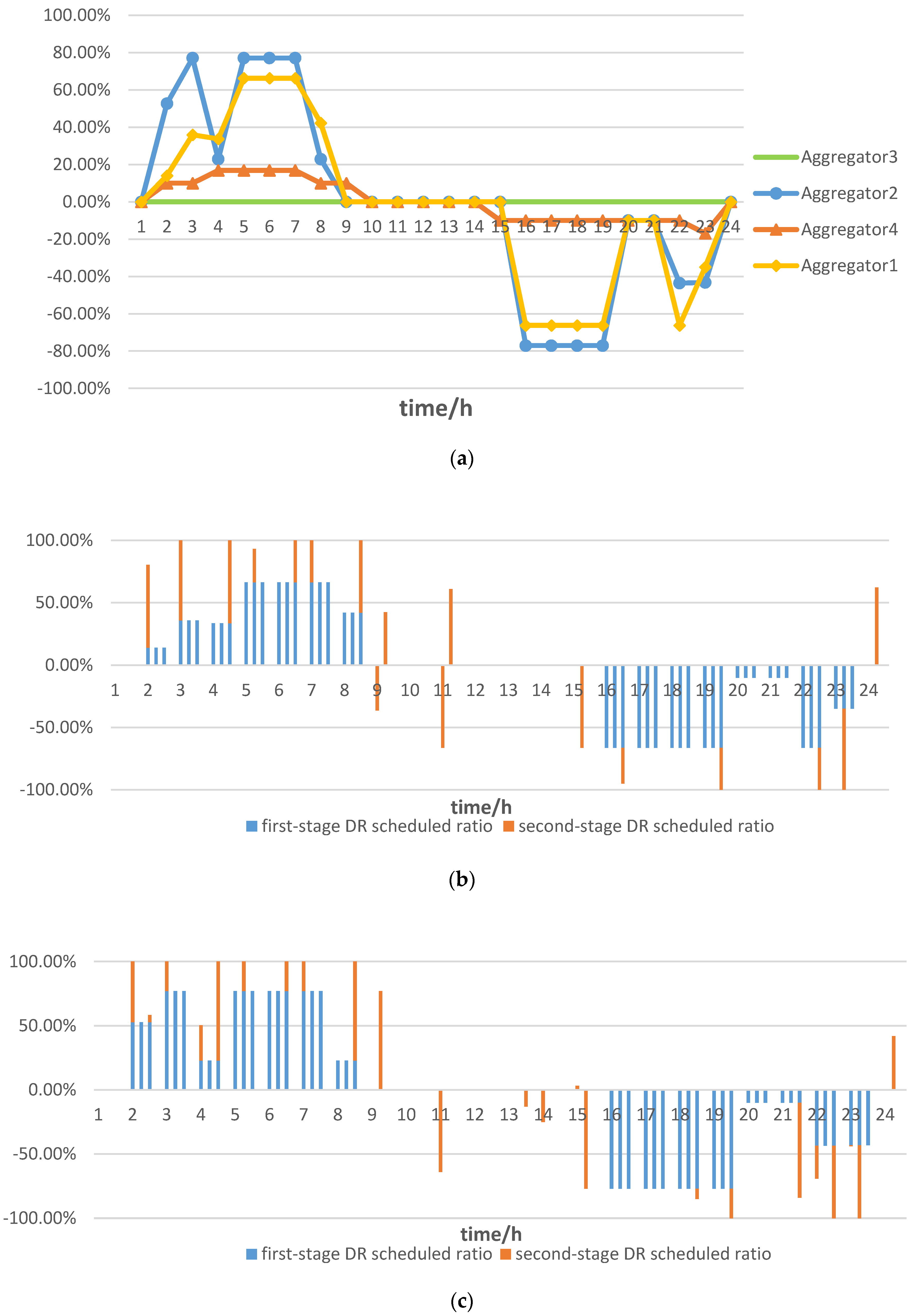
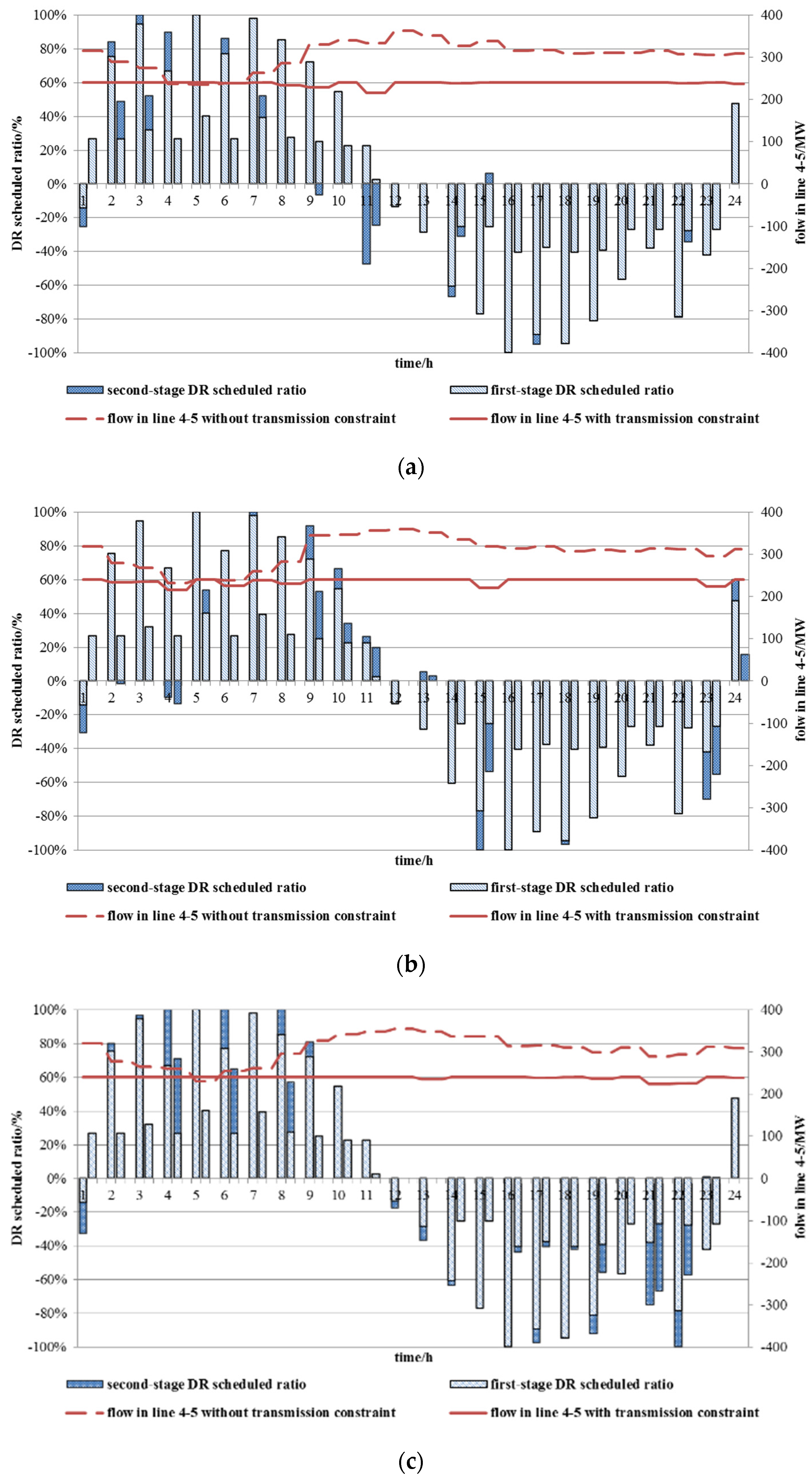
(3) Results Considering Transmission Constraints

The results with transmission constraints are discussed in this subsection to investigate the impact on DR flexible scheduling. Table 6 shows the costs under different DR scheduling modes when transmission constraints are considered.

Table 6. DR scheduling modes impact on cost (wind power profile 1): With transmission constraint.

Mode	ODR	FDR	SDR	F&SDR (Proposed Model)
Total Cost (103$)	Base (1141.40)	−508.76	−525.95	−556.52
Generation Cost (103$)	Base (529.54)	+30.92	+35.71	+35.58
Start-up Cost (103$)	Base (0.3)	+0	+0	+0
Wind Curtailment Cost (103$)	Base (2.80)	−2.76	−2.80	−2.80
Load not Served Cost (103$)	Base (608.79)	−551.54	−605.67	−605.67
DR Capacity Cost (103$)	Base (0)	+2.1	+2.1	+2.1
DR Operating Cost (103$)	Base (0)	+12.50	+44.69	+14.24

Table 6. DR scheduling modes impact on cost (wind power profile 1): With transmission constraint.

Mode	ODR	FDR	SDR	F&SDR (Proposed Model)
Total Cost (103$)	Base (1141.40)	−508.76	−525.95	−556.52
Generation Cost (103$)	Base (529.54)	+30.92	+35.71	+35.58
Start-up Cost (103$)	Base (0.3)	+0	+0	+0
Wind Curtailment Cost (103$)	Base (2.80)	−2.76	−2.80	−2.80
Load not Served Cost (103$)	Base (608.79)	−551.54	−605.67	−605.67
DR Capacity Cost (103$)	Base (0)	+2.1	+2.1	+2.1
DR Operating Cost (103$)	Base (0)	+12.50	+44.69	+14.24

Because the network capability to accommodate and transport power influences wind power penetration [39], all concerned costs (especially the load not served cost) in the case of all four modes in Table 6 increase with respect to the values in Table 3 when transmission constraints are considered because congestion causes expensive units to be dispatched and results in increased load curtailment. The proposed mode still has the lowest cost, as illustrated in Table 6. The proposed mode increases cost savings and creates a higher level of system balance when compared to the case without transmission constraints (Table 3).

Another simulation is performed to calculate the cost of the scheduling and the dispatch rate of the DR resource using the new wind power data containing 5 scenarios in Figure 7. According to these scenarios of wind power data, the DR scheduling modes impact on cost is shown in Table 7.

By comparing Table 7 with Table 6, it can be seen that when the wind power scene is extended to 5 scenarios, the law in the original manuscript is maintained. After scheduling DR resources, wind curtailment and load shedding decreased significantly. This result shows that DR resources are beneficial in accommodating wind power. Furthermore, by comparing the three scheduling modes, that is, DR scheduled only in the first stage, DR scheduled only in the second stage and DR scheduled flexibly in two stages (the model proposed in this paper), the total cost and wind power curtailment of the last mode is lowest. The calculation is the same as in Table 4.

Figure 7. New wind power data containing five scenarios.

Figure 7. New wind power data containing five scenarios.

Table 7. DR scheduling modes impact on cost (wind power profile two and five scenarios): With transmission constraint.

Mode	ODR	FDR	SDR	F&SDR (Proposed Model)
Total Cost (103$)	Base (976.590)	−427.33	−406.55	−431.16
Generation Cost (103$)	Base (492.66)	+29.71	+30.51	+29.81
Start-up Cost (103$)	Base (0.6)	−0.3	−0.3	−0.3
Wind Curtailment Cost (103$)	Base (1.14)	−1.14	−1.14	−1.14
Load not Served Cost (103$)	Base (482.19)	−468.03	−472.13	−472.13
DR Capacity Cost (103$)	Base (0)	+2.1	+2.1	+2.1
DR Operating Cost (103$)	Base (0)	+10.34	+34.41	+10.51

Table 7. DR scheduling modes impact on cost (wind power profile two and five scenarios): With transmission constraint.

Mode	ODR	FDR	SDR	F&SDR (Proposed Model)
Total Cost (103$)	Base (976.590)	−427.33	−406.55	−431.16
Generation Cost (103$)	Base (492.66)	+29.71	+30.51	+29.81
Start-up Cost (103$)	Base (0.6)	−0.3	−0.3	−0.3
Wind Curtailment Cost (103$)	Base (1.14)	−1.14	−1.14	−1.14
Load not Served Cost (103$)	Base (482.19)	−468.03	−472.13	−472.13
DR Capacity Cost (103$)	Base (0)	+2.1	+2.1	+2.1
DR Operating Cost (103$)	Base (0)	+10.34	+34.41	+10.51

Table 8 represents the average proportion of DR scheduled in each stage considering transmission constraints.

Table 8 shows DR resources from three aggregators (1, 3 and 5) dispatched in both stages. However, if transmission constraints are not considered (Table 8), there is only one aggregator 3 dispatched. In theory, DR resources with less flexibility but lower cost will be dispatched more in the first stage, those with more flexibility but higher cost will be dispatched in the first stage, and those with lower cost in the second stage will be dispatched in the second stage. This also explains why the proposed model will flexibly allocate DR in two stages according to the system requirement based on the coupling relationship of DR resources (as the case of Table 8).

Table 8. Average absolute proportion of DR scheduled in each stage for each aggregator: With transmission constraint.

DR Aggregators	First Stage	Second_s1	Second_s2	Second_s3
1	49.67%	5.12%	1.58%	9.44%
2	74.27%	0%	0%	0.13%
3	76.67%	6.67%	9.17%	6.67%
4	90.93%	0%	0%	0%
5	21.81%	16.37%	24.47%	32.82%

Table 8. Average absolute proportion of DR scheduled in each stage for each aggregator: With transmission constraint.

DR Aggregators	First Stage	Second_s1	Second_s2	Second_s3
1	49.67%	5.12%	1.58%	9.44%
2	74.27%	0%	0%	0.13%
3	76.67%	6.67%	9.17%	6.67%
4	90.93%	0%	0%	0%
5	21.81%	16.37%	24.47%	32.82%

Furthermore, compared to the results in Table 4, almost every aggregator in Table 8 has a higher proportion scheduled, especially in the first stage, which may result from a different power flow distribution in the case of different scenarios, as limited by constraint (3).

Figure 8 illustrates the proportion of DR scheduled in two stages and the flow of lines 4–5 for 24 h without transmission constraint consideration. The proportion of DR scheduled in the first and second stages is calculated by:

$${\displaystyle \sum _{d=1}^{N_d}(d{1}_{d,t}^{+}+d{1}_{d,t}^{-})}/{\displaystyle \sum _{d=1}^{N_d}D{R}_d^{\max }}\mathrm{and}{\displaystyle \sum _{d=1}^{N_d}(d{2}_{d,t,s}^{+}+d{2}_{d,t,s}^{-})}/{\displaystyle \sum _{d=1}^{N_d}D{R}_d^{\max }}$$

The 24 pairs of bars in Figure 8a–c represent the proportion of DR scheduled (on the left axis) and the left/right bars stand for with/without transmission constraints, respectively. Within columns, there are up to two colors, indicating the DR scheduled level in two stages, which are read off of the left axis. The dished/solid lines indicate the flow of lines 4–5 (on the right axis) with/without transmission constraints for all three scenarios. The reason the impact of the wind scenarios has very little impact on the scheduling of DR is as follows: in Figure 8 the scheduling of DR in the first stage (bar with light color) is the same in all scenarios, and the first-stage DR is dispatched much more than the second-stage DR (bar with dark color).However, the scheduling of the second-stage DR varies, for example, at 11 h the second-stage DR scheduled ratio with transmission constraint (left bar) is −48%, 4% and 0%.This difference results from the different wind power output in all scenarios. When considering the new wind power data containing five scenarios, the average absolute proportion of DR scheduled flexibly in two-stages for each aggregator is shown in Table 9.

Figure 8. Proportion of DR scheduled in two stages and power flow of lines 4–5. In the transmission constraint case, the flow in lines 4–5 is limited to 240 MW during most hours of all scenarios due to congestion. Meanwhile, more DR resources are dispatched in the first stage (DR on a day-ahead basis, which has lower operating cost) rather than in the second stage (DR on an intra-day basis, which has higher operating cost). (a) Results of scenario 1; (b) Results of scenario 2; (c) Results of scenario 3.

Figure 8. Proportion of DR scheduled in two stages and power flow of lines 4–5. In the transmission constraint case, the flow in lines 4–5 is limited to 240 MW during most hours of all scenarios due to congestion. Meanwhile, more DR resources are dispatched in the first stage (DR on a day-ahead basis, which has lower operating cost) rather than in the second stage (DR on an intra-day basis, which has higher operating cost). (a) Results of scenario 1; (b) Results of scenario 2; (c) Results of scenario 3.

Table 9. Average absolute proportion of DR scheduled in each stage for each aggregator (five scenarios): With transmission constraint.

DR Aggregators	First_stage	Second_s1	Second_s2	Second_s3	Second_s4	Second_s5
1	35.15%	0.51%	0.48%	0.48%	0.48%	2.55%
2	59.44%	0%	0%	0%	0%	0%
3	70.83%	4.17%	6.46%	4.17%	5.40%	4.17%
4	83.33%	0%	0%	0%	0%	0%
5	28.65%	4.84%	3.21%	19.19%	3.96%	7.25%

Table 9. Average absolute proportion of DR scheduled in each stage for each aggregator (five scenarios): With transmission constraint.

DR Aggregators	First_stage	Second_s1	Second_s2	Second_s3	Second_s4	Second_s5
1	35.15%	0.51%	0.48%	0.48%	0.48%	2.55%
2	59.44%	0%	0%	0%	0%	0%
3	70.83%	4.17%	6.46%	4.17%	5.40%	4.17%
4	83.33%	0%	0%	0%	0%	0%
5	28.65%	4.84%	3.21%	19.19%	3.96%	7.25%

By comparing Table 9 with Table 8, it can be seen that when the wind power scene is extended to 5 scenarios, the average absolute proportions of DR scheduled in different stages are similar, which is consistent with the result of Table 8.

Figure 9 shows the generator output of scenario1 for 24 h without transmission constraints. The left bar of every pair in Figure 9 represents the generation output of the generators in the system with transmission constraints, whereas the right bar is the output without transmission constraints.

Figure 8a–c show that in the transmission constraint case, the flow in lines 4–5 is limited to 240 MW during most of hours due to congestion. Meanwhile, the results in Figure 9 show that the generation output of G3 increases and G5 decreases when the transmission constraint is considered because a limited amount of power provided by generators located on the generation side (G5 in this case) can be imported because of the transmission congestion in lines 4–5. Congestion causes part of the load at a certain bus to be met locally. To solve these problems, load curtailment or shifting can be adopted when DR is available. On the other hand, the generator with higher cost but located at the load center (G3 in this case) must increase its output level to maintain the power balance locally, especially during peak load hours (12 p.m. to 10 p.m., Figure 3). However, conventional generators have physical operation constraints, such as the ramp rate, so the generator must be turned on in advance to ramp up to the required output level at a given time. As shown in Figure 9, considering transmission constraints, G3 has to start earlier such that it can achieve significantly high output level during peak time. However, the early start of G3 leads to greater generation during valley time and requires higher demand growth to consume the extra generation, which results in a significant increase of DR resources dispatched, as shown in Table 8.

Although the flows of the wind power scenarios are slightly different, congestion occurs in all three scenarios, as shown in Figure 8. Because the objective of stochastic programming is to minimize the expected total cost of all scenarios, more DR resources are dispatched in the first stage (DR on a day-ahead basis, which has lower operating cost) rather than in the second stage (DR on an intra-day basis, which has higher operating cost) to satisfy the common requirement of all scenarios.

In short, load shifting from peak to valley is beneficial to address challenges resulting from transmission congestion and the physical restrictions of generators, so that system reliability and stability can be maintained in addition to accommodating much more renewable energy. This means that co-optimization of the generation and demand resources could alleviate the impact of transmission congestion and renewable energy fluctuations through DR scheduling. From the above analysis, it is evident that congestion may cause much more DR resources to be dispatched in the first stage. Thus, it is recommended that more DR resources in the first stage (DR on a day-ahead basis) should be dispatched when congestion is expected.

Furthermore, the results in Table 8 illustrate that the cost is still the most critical factor affecting DR scheduling when transmission constraints are considered, as shown in Table 3 (without transmission constraints). DR aggregator 4 has the highest proportion of DR resources scheduled in the first stage because it has the lowest operation cost ($2/MWh); then, DR aggregator 3 stands in the second stage because its costs ($5/MWh) are a little higher than DR aggregator 4. Likewise are the DR resources scheduled in the second stage.

Figure 9. Generation output of scenario1 without transmission constraint. The generation output of G3 increases and G5 decreases when the transmission constraint is considered. Meanwhile, G3 has to start earlier such that it can achieve significantly high output level during the peak time. (a) Generation output in scenario 1; (b) Generation output in scenario 2; (c) Generation output in scenario 3.

Figure 9. Generation output of scenario1 without transmission constraint. The generation output of G3 increases and G5 decreases when the transmission constraint is considered. Meanwhile, G3 has to start earlier such that it can achieve significantly high output level during the peak time. (a) Generation output in scenario 1; (b) Generation output in scenario 2; (c) Generation output in scenario 3.

4.2. IEEE 118 Case

4.2.1. Data Assumption

The load profile of Figure 3 with scaled peak values is adopted to match the load level at each bus of the IEEE 118-bus system. The wind power is located at Bus 1, and the output curve in Figure 4 remains unchanged. DR resources are located at Bus 59. Table 10 shows the DR aggregator characteristics adopted in this case. There are five branch thermal limits added to the transmission system.

Table 10. DR aggregator characteristics in IEEE 118 case.

DR Aggregators	$D{R}_d^{\max }$ (MW)	$D{R}_d^{\min }$ (MW)	${\mathit{MDT}}_d$ (h)	$E{c}_{d1}^{\pm }$/$E{c}_{d2}^{\pm }$ ($/MWh)	$C{c}_d$ ($/MW)
1	42	4.2	4	8/20	15
2	30	3.0	4	6/25	15
3	30	3.0	8	5/16	15
4	42	4.2	8	2/23	15
5	24	2.4	1	10/15	15

Table 10. DR aggregator characteristics in IEEE 118 case.

DR Aggregators	$D{R}_d^{\max }$ (MW)	$D{R}_d^{\min }$ (MW)	${\mathit{MDT}}_d$ (h)	$E{c}_{d1}^{\pm }$/$E{c}_{d2}^{\pm }$ ($/MWh)	$C{c}_d$ ($/MW)
1	42	4.2	4	8/20	15
2	30	3.0	4	6/25	15
3	30	3.0	8	5/16	15
4	42	4.2	8	2/23	15
5	24	2.4	1	10/15	15

4.2.2. Results and Discussion

With the lowest total costs, F&SDR (4.57 × 10⁶ $) performs the best compared with ODR (4.67 × 10⁶ $), FDR (4.58 × 10⁶ $) and SDR (4.58 × 10⁶ $). Table 11 presents the average absolute proportion of DR scheduled in each stage for each aggregator and confirms that cost is the most critical factor affecting DR scheduling. The DR aggregators with lower costs (aggregator 4 in the first stage and aggregator 5 in the second stage) are dispatched more frequently.

Table 11. Average absolute proportion of DR scheduled in each stage for each aggregator of the IEEE 118 case with transmission constraints.

DR Aggregators	First_s	Second_s1	Second_s2	Second_s3
1	8.75%	2.08%	2.08%	2.41%
2	10.83%	0%	0%	0%
3	15.42%	2.08%	3.07%	6.25%
4	66.67%	0%	0%	0%
5	4.17%	4.17%	4.17%	8.33%

Table 11. Average absolute proportion of DR scheduled in each stage for each aggregator of the IEEE 118 case with transmission constraints.

DR Aggregators	First_s	Second_s1	Second_s2	Second_s3
1	8.75%	2.08%	2.08%	2.41%
2	10.83%	0%	0%	0%
3	15.42%	2.08%	3.07%	6.25%
4	66.67%	0%	0%	0%
5	4.17%	4.17%	4.17%	8.33%

5. Conclusions

This paper explores a new approach to flexibly schedule DR resources based on a two-stage stochastic programming process to maximize the effectiveness of DR on wind power integration. The contribution of this work can be summarized as below:

(1)

The tight coupling characteristics of specific DR resources on available time and capacity are considered in the proposed stochastic model. Specifically, if sufficient incentives are paid to consumers, some DR resources can be scheduled both in the first stage as resources on a day-ahead basis to integrate the wind power with lower uncertainty and in the second stage as resources on an intra-day basis to integrate the wind power with higher uncertainty. Flexible DR scheduling can achieve the maximal DR values with the minimal cost, combining the cost advantage of DR on a day-ahead basis and the flexibility advantage of DR on an intra-day basis, which is beneficial with high wind power penetration.

(2)

The responsive cost rather than the characteristics of flexibility, including “minimum on-site time” and “minimum responsive capacity”, is the most critical factor, but “minimum onsite hours” plays a more important role when only the characteristic of flexibility is considered.

(3)

The first stage DR should be dispatched more frequently when transmission congestion is expected to occur.

Notwithstanding the contributions of our paper, there remain some points to be improved in the future work: since the wind power output is characterized by intermittency, volatility and randomness, this paper only took two wind power output profiles as well as the corresponding three or five scenarios into account. In future work we may develop a more detailed model, considering more types of wind power output and scenarios. We will focus on finding a solution that balances the cost of unhedged uncertainty from the SUC against the wind power prediction error inherent in the interval unit commitment formulation.

References

1. Wang, B.; Hobbs, B.F. A flexible ramping product: Can it help real-time dispatch markets approach the stochastic dispatch ideal. Electr. Power Syst. Res. 2014, 109, 128–140. [Google Scholar] [CrossRef]
2. Chong, C.; Ni, W.; Ma, L.; Liu, P.; Li, Z. The use of energy in Malaysia: Tracing energy flows from primary source to end use. Energies 2015, 8, 2828–2866. [Google Scholar] [CrossRef]
3. Kiliccote, S.; Sporborg, P.; Sheik, I. Integrating Renewable Resources in California and the Role of Automated Integrating Renewable Resources in California and the Role of Automated Demand Response; Lawrence Berkeley National Laboratory: Berkeley, CA, USA, 2010. [Google Scholar]
4. Li, F.; Wei, Y. A probability-driven multilayer framework for scheduling intermittent renewable energy. IEEE Trans. Sustain. Energy 2012, 3, 455–461. [Google Scholar] [CrossRef]
5. Gu, W.; Yu, H.; Liu, W.; Zhu, J.; Xu, X. Demand response and economic dispatch of power systems considering large-scale plug-in hybrid electric vehicles/electric vehicles (PHEVs/EVs): A review. Energies 2013, 6, 4394–4417. [Google Scholar] [CrossRef]
6. Dietrich, K.; Latorre, J.M.; Olmos, L. Demand response in an isolated system with high wind integration. IEEE Trans. Power Syst. 2012, 27, 20–29. [Google Scholar] [CrossRef]
7. Sioshansi, R. Evaluating the impacts of real-time pricing on the cost and value of wind generation. IEEE Trans. Power Syst. 2010, 25, 741–748. [Google Scholar] [CrossRef]
8. Javad, S.; Mohammad, H.J. Economic evaluation of demand response in power systems with high wind power penetration. J. Renew. Sustain. Energy 2014, 6, 1–17. [Google Scholar]
9. Sioshansi, R.; Short, W. Evaluating the impacts of real-time pricing on the usage of wind generation. IEEE Trans. Power Syst. 2009, 24, 516–524. [Google Scholar] [CrossRef]
10. Madaeni, S.H.; Sioshansi, R. Using demand response to improve the emission benefits of wind. IEEE Trans. Power Syst. 2013, 28, 1385–1394. [Google Scholar] [CrossRef]
11. Amirhossein, K.; Mohsen, K. Optimal generation dispatch incorporating wind power and responsive loads: A chance-constrained framework. J. Renew. Sustain. Energy 2015, 7, 1–21. [Google Scholar]
12. De Jonghe, C.; Hobbs, B.F.; Belmans, R. Value of demand response for wind integration in daily power generation scheduling: Unit commitment modeling with price responsive load. In Proceedings of the USAEE/IAEE North American Conference, Washington, DC, USA, 9–12 October 2011.
13. Madaeni, S.H.; Sioshansi, R. The impacts of stochastic programming and demand response on wind integration. Energy Syst. 2013, 4, 109–124. [Google Scholar] [CrossRef]
14. Bahreyni, S.A.H.; Khorsand, M.A.; Jadid, S. A stochastic unit commitment in power systems with high penetration of smart grid technologies. In Proceedings of the 2nd Iranian Conference on Smart Grids (ICSG), Tehran, Iran, 15–17 May 2012.
15. Falsafi, H.; Zakariazadeh, A.; Jadid, S. The role of demand response in single and multi-objective wind-thermal generation scheduling: A stochastic programming. Energy 2014, 64, 853–867. [Google Scholar] [CrossRef]
16. Torres, D.; Crichigno, J.; Padilla, G.; Rivera, R. Scheduling coupled photovoltaic, battery and conventional energy sources to maximize profit using linear programming. Renew. Energy 2014, 72, 284–290. [Google Scholar] [CrossRef]
17. Parvania, M.; Fotuhi-Firuzabad, M. Demand response scheduling by stochastic SCUC. IEEE Trans. Smart Grid 2010, 1, 89–98. [Google Scholar] [CrossRef]
18. Wang, J.; Botterud, A.; Miranda, V.; Monteiro, C.; Sheble, G. Impact of wind power forecasting on unit commitment and dispatch. In Proceedings of the 8th International Workshop Large-Scale Integration of Wind Power into Power Systems, Bremen, Germany, 14–15 October 2009.
19. Gyamfi, S.; Krumdieck, S.; Urmee, T. Residential peak electricity demand response-highlights of some behavioural issues. Renew. Sustain. Energy Rev. 2013, 25, 71–77. [Google Scholar] [CrossRef]
20. Benefits of Demand Response in Electricity Markets and Recommendations for Achieving Them: A Report to the United States Congress Pursuant to Section 1252 of the Energy Policy Act of 2005; Department of Energy: Washington, DC, USA, 2006.
21. Lei, W.; Shahidehpour, M.; Li, Z. Comparison of scenario-based and interval optimization approaches to stochastic SCUC. IEEE Trans. Power Syst. 2012, 27, 913–921. [Google Scholar]
22. Wang, J.; Shahidehpour, M.; Li, Z. Security-constrained unit commitment with volatile wind power generation. IEEE Trans. Power Syst. 2008, 23, 1319–1327. [Google Scholar] [CrossRef]
23. Yuan, Y.; Chung, S. Dispatch of direct load control using dynamic programming. IEEE Trans. Power Syst. 1991, 6, 1056–1061. [Google Scholar] [CrossRef]
24. Strbac, G. Demand side management: Benefits and challenges. Energy Policy 2008, 36, 4419–4426. [Google Scholar] [CrossRef]
25. Pennsylvania-New Jersey-Maryland (PJM). PJM Training Materials (LMP101). Available online: http://www.pjm.com/Globals/Training/Courses/ip-lmp-ftr-101.aspx/ (accessed on 26 November 2015).
26. University of Washington. Power System Test Case Archive. Available online: http://www.ee.washington.edu/research/pstca/ (accessed on 25 November 2015).
27. Energy, G. Western Wind and Solar Integration Study; National Renewable Energy Laboratory (NREL): Golden, CO, USA, 2010. [Google Scholar]
28. Gröwe-Kuska, N.; Heitsch, H.; Römisch, W. Scenario reduction and scenario tree construction for power management problems. In Proceedings of the 2003 IEEE Bologna PowerTech Conference, Bologna, Italy, 23–26 June 2003.
29. Ma, X.; Sun, Y.; Fang, H. Scenario generation of wind power based on statistical uncertainty and variability. IEEE Trans. Sustain. Energy 2013, 4, 894–904. [Google Scholar] [CrossRef]
30. Koc, A.; Ghosh, S. Optimal scenario tree reductions for the stochastic unit commitment problem. In Proceedings of the 2012 Winter Simulation Conference (WSC), Berlin, Germany, 9–12 December 2012; pp. 1–12.
31. Sumaili, J.; Keko, H.; Miranda, V. Finding representative wind power scenarios and their probabilities for stochastic models. In Proceedings of the 2011 16th International Conference on Intelligent System Application to Power Systems (ISAP), Hersonissos, Greece, 25–28 September 2011; pp. 1–6.
32. Barth, R. Deliverable D6.2 (b)—Documentation Methodology of the Scenario Tree Tool, Institute of Energy Economics and the Rational Use of Energy (IER); University of Stuttgart: Stuttgart, Germany, 2006. [Google Scholar]
33. Wang, B.; Dennice, F.G.; Liu, X.; Yuan, C. Optimal siting and sizing of demand response in a transmission constrained system with high wind penetration. Int. J. Electr. Power Energy Syst. 2015, 68, 71–80. [Google Scholar] [CrossRef]
34. Papavasiliou, A.; Oren, S. A stochastic unit commitment model for integrating renewable supply and demand response. In Proceedings of the IEEE Power and Energy Society General Meeting 2012, San Diego, CA, USA, 2012; pp. 1–6.
35. Gayme, D.; Topcu, U. Optimal power flow with large-scale storage integration. IEEE Trans. Power Syst. 2013, 28, 709–717. [Google Scholar] [CrossRef]
36. Energy, G.E. Western Wind and Solar Integration Study. Subcontract Technical Representative Report NREL/SR-550–47434. 2010. Available online: http://www.osti.gov/bridge/ (accessed on 12 December 2014). [Google Scholar]
37. Papavasiliou, A. Coupling Renewable Energy Supply with Deferrable Demand; University of California: Berkeley, CA, USA, 2011. [Google Scholar]
38. Dvorkin, Y.; Pandzic, H.; Ortega-Vazquez, M. A hybrid stochastic/interval approach to transmission-constrained unit commitment. IEEE Trans. Power Syst. 2015, 30, 621–631. [Google Scholar] [CrossRef]
39. Hamidi, V.; Li, F.; Yao, L. Value of wind power at different locations in the grid. IEEE Trans. Power Deliv. 2011, 26, 526–537. [Google Scholar] [CrossRef]