
Multi-Objective Optimization Design for Indirect Forced-Circulation Solar Water Heating System Using NSGA-II


Abstract
:1. Introduction
2. Mathematical Models of SWH System
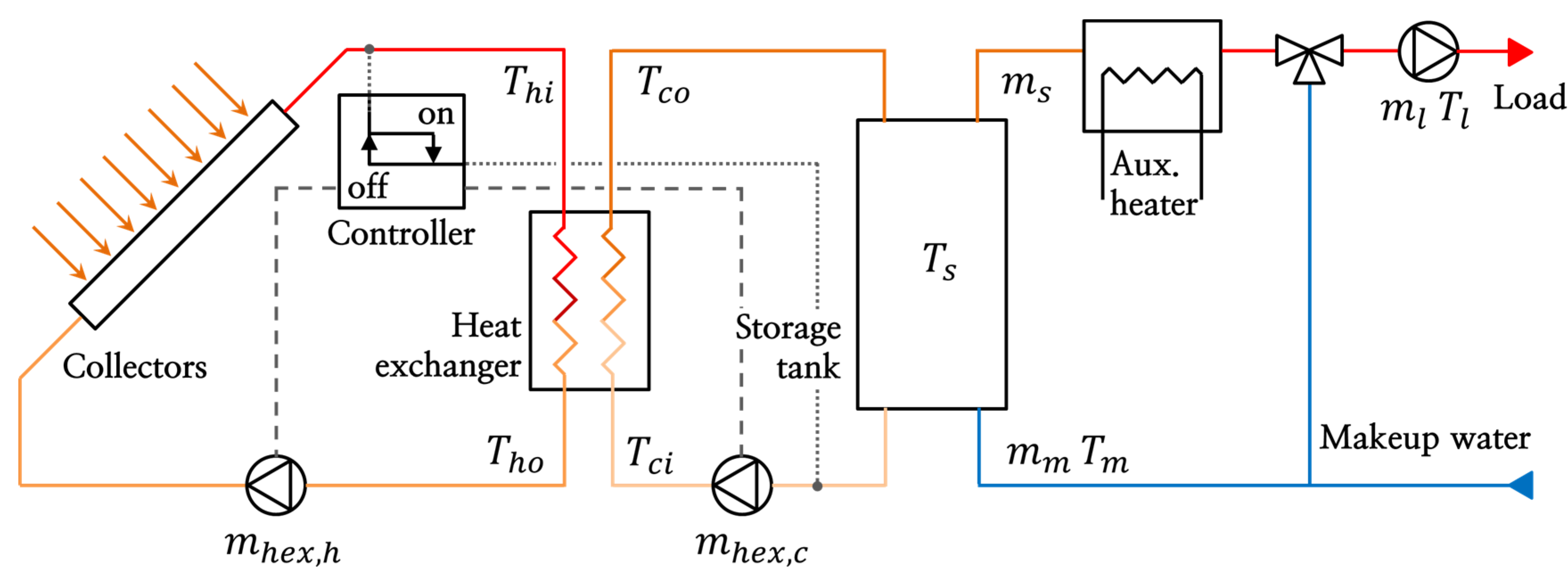
2.1. Flat-Plate Solar Collector
2.2. Heat Exchanger
2.3. Storage Tank
2.4. Auxiliary Heater
2.5. Circulation Pump
2.6. Energy Performance of SWH System
3. Multi-Objective Optimization Method of SWH System
3.1. Decision Variable
3.2. Objective Functions
3.3. Constraint Conditions
- (a)
- The limits of , , , and are set automatically as the number of types in the inputted data tables of each component.
- (b)
- The limits of and are not set because to be a feasible solution, any decision vector should be subject to the inequality constraints (c) and (d) mentioned below. The number of storage tanks and heat exchangers is taken as one because this is the common configuration of indirect forced-circulation SWH systems in South Korea.
- (c)
- To make the solutions obtained by the optimization method reasonable for practical designs, space should be available to install solar collectors. This is defined as follows:
- (d)
- If solar energy is not available, the auxiliary heaters should be capable of providing the required hot water load, as shown below:
- (e)
- The slope of the collector array is given as follows:
- (f)
- (g)
- Increasing the NTU value of a heat exchanger beyond three or four usually results in only an insignificant improvement in effectiveness compared to the increase in the cost. Therefore, the NTU of the heat exchanger should be subject to the following constraint:
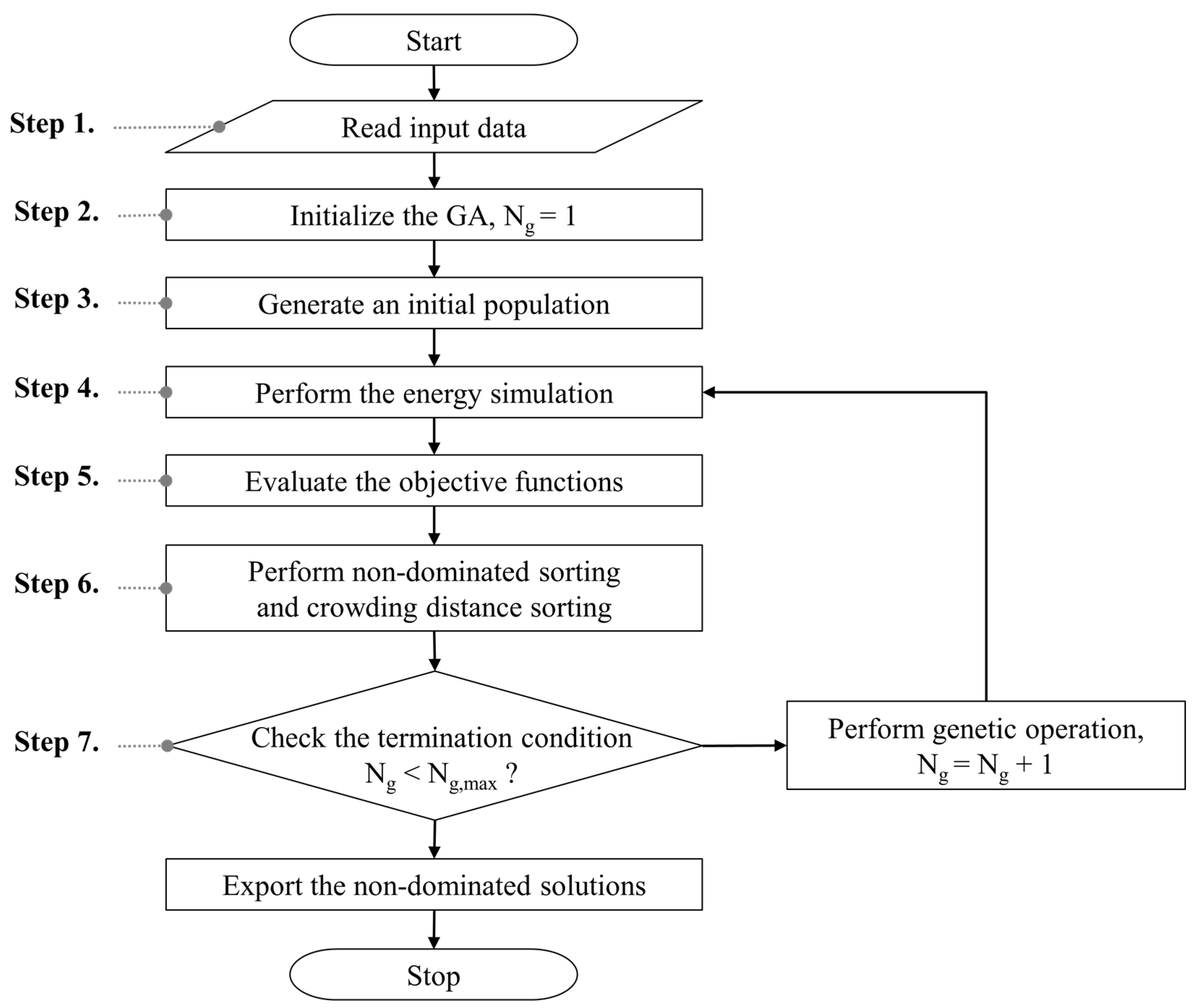
3.4. Application of NSGA-II to Optimize SWH System
4. Simulation Results and Discussion
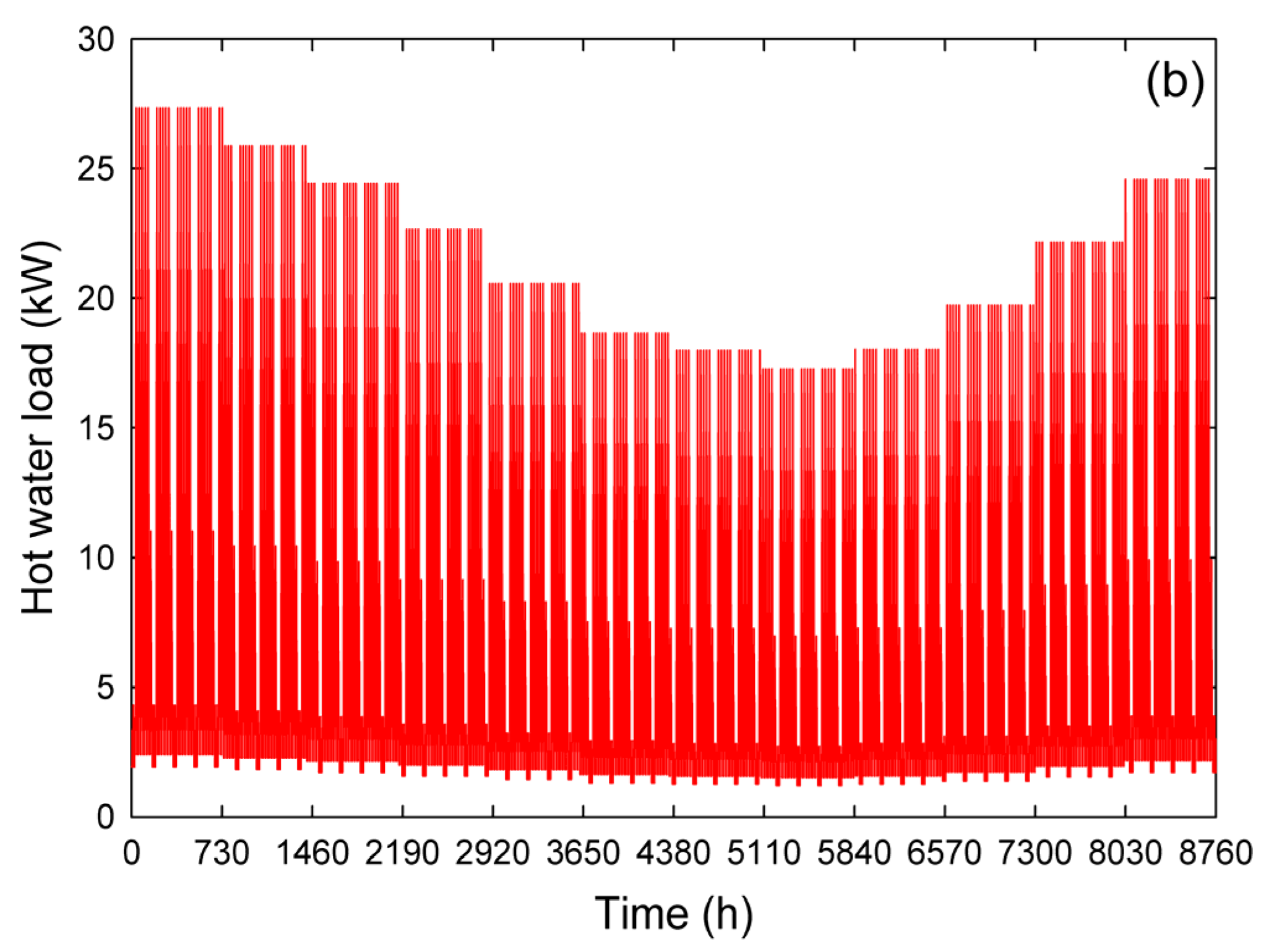
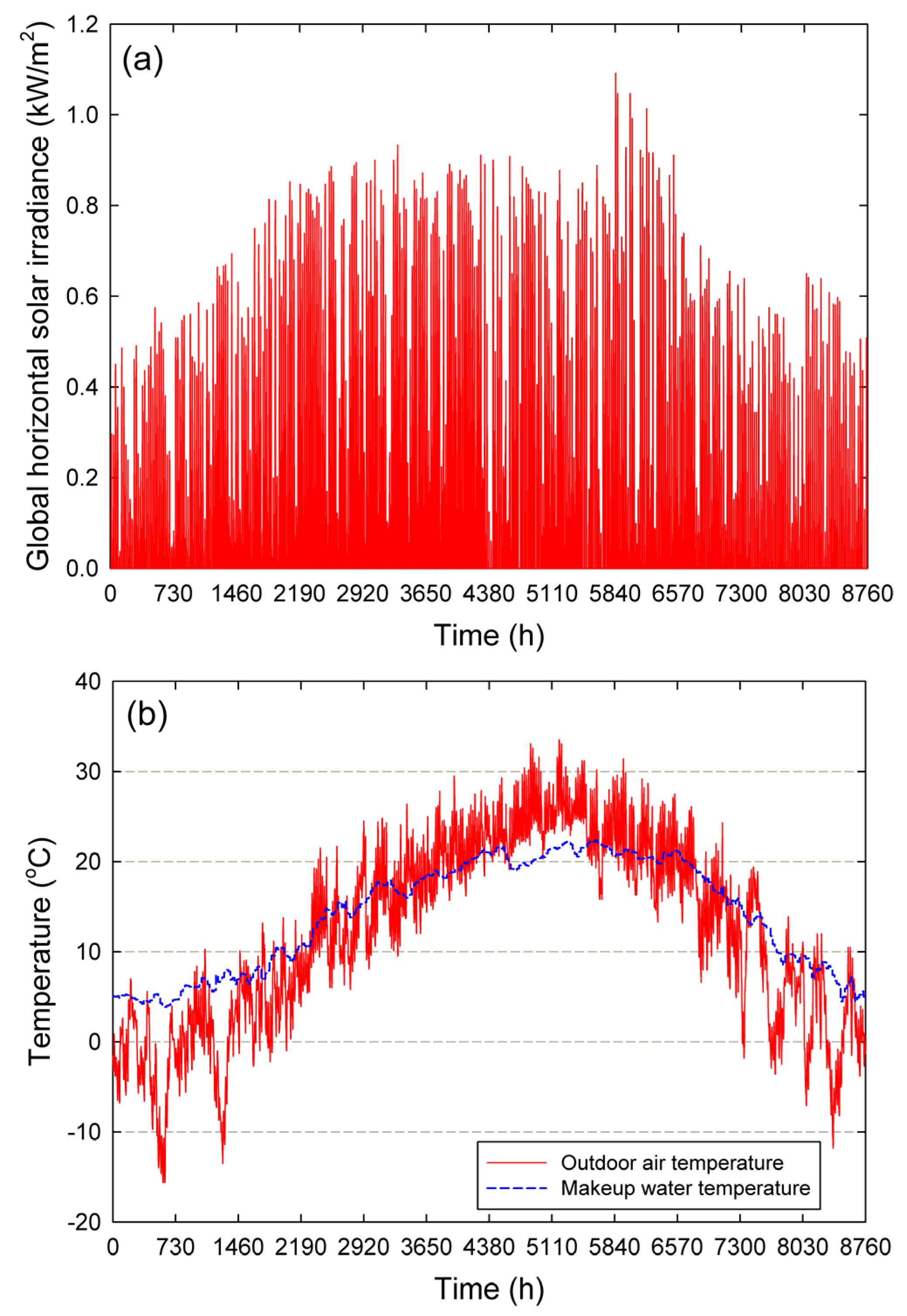
4.1. Simulation Parameters


| Parameter | Description | Value |
|---|---|---|
| Azimuth of collector array (°) | 0 | |
| Meridian altitude in winter (°) | 29 | |
| Desired hot water temperature (°C) | 60 | |
| Maximum allowable storage tank temperature (°C) | 100 | |
| Temperature of environment surrounding storage tank (°C) | 20 | |
| Maximum number of collectors in series (ea.) | 6 | |
| Specific heat of collector fluid (J/kg·°C) | 3843 | |
| Specific heat of water (J/kg·°C) | 4153 | |
| Density of collector fluid (kg/m3) | 1032 | |
| Density of water (kg/m3) | 991 | |
| Ground reflectance (-) | 0.2 | |
| Upper deadband temperature difference of DTC (°C) | 8 | |
| Lower deadband temperature difference of DTC (°C) | 2 | |
| Pumping efficiency of circulation pump (%) | 60 | |
| Motor efficiency of circulation pump (%) | 80 | |
| Head of pump on hot side of heat exchanger (m) | 80 | |
| Head of pump on cold side of heat exchanger (m) | 15 | |
| Head of pump on load side of SWH system (m) | 80 | |
| Planning period (years) | 40 | |
| Real discount rate (%) | 2.91 | |
| Electricity cost escalation rate (%) | 4.00 | |
| Gas cost escalation rate (%) | 4.00 | |
| Maximum capacity available to receive subsidy cost (m2) | 500 | |
| Area available to install solar collectors (m2) | 600 | |
| Supplementary cost ratio against purchase cost (%) | 30 | |
| Maintenance cost ratio against initial cost (%) | 1.5 | |
| Subsidy cost ratio against initial cost (%) [42] | 50 |
| Classification | Value | ||
|---|---|---|---|
| Electricity | Basic charge | 6160 | |
| Energycharge (KRW/kW·h) | Summer (June, July, and August) | 105.7 | |
| Spring/fall (March, April, May, September, and October) | 65.2 | ||
| Winter (November, December, January, and February) | 92.3 | ||
| LNG | Energycharge (KRW/MJ) | Summer (May, June, July, August, and September) | 19.26 |
| Spring/fall (April, October, and November) | 19.28 | ||
| Winter (December, January, February, and March) | 19.46 | ||
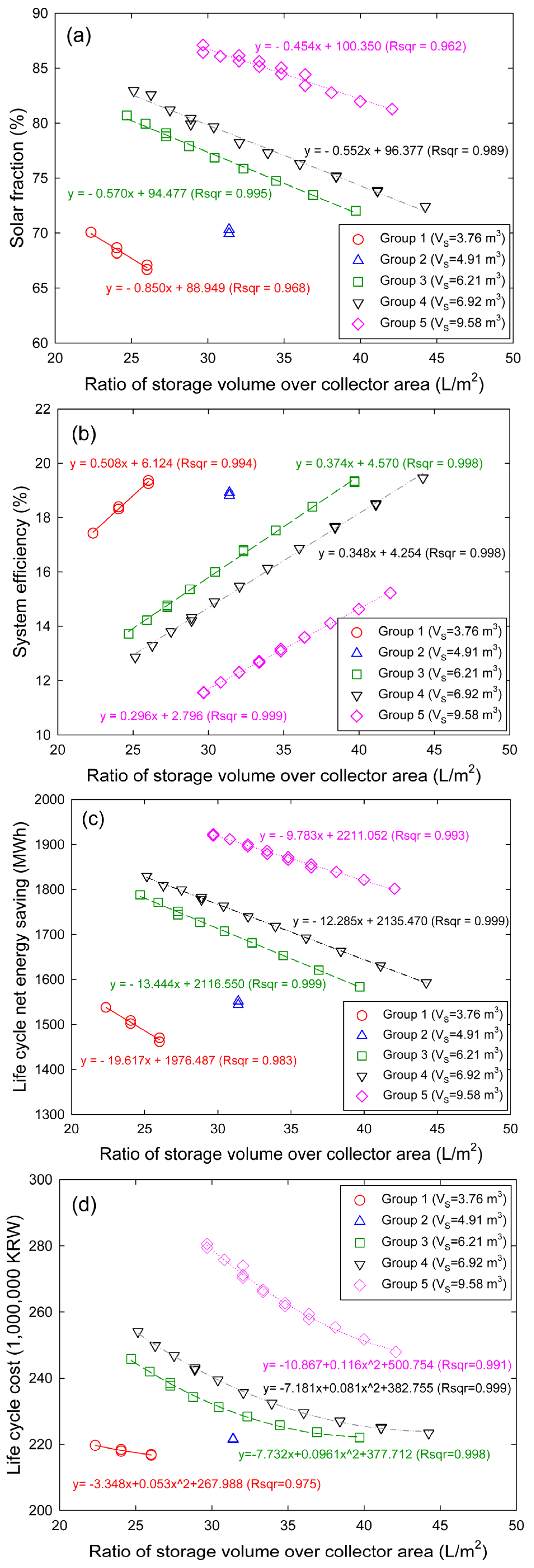
4.2. Multi-Objective Optimization Results


| Parameter | Classification | |||
|---|---|---|---|---|
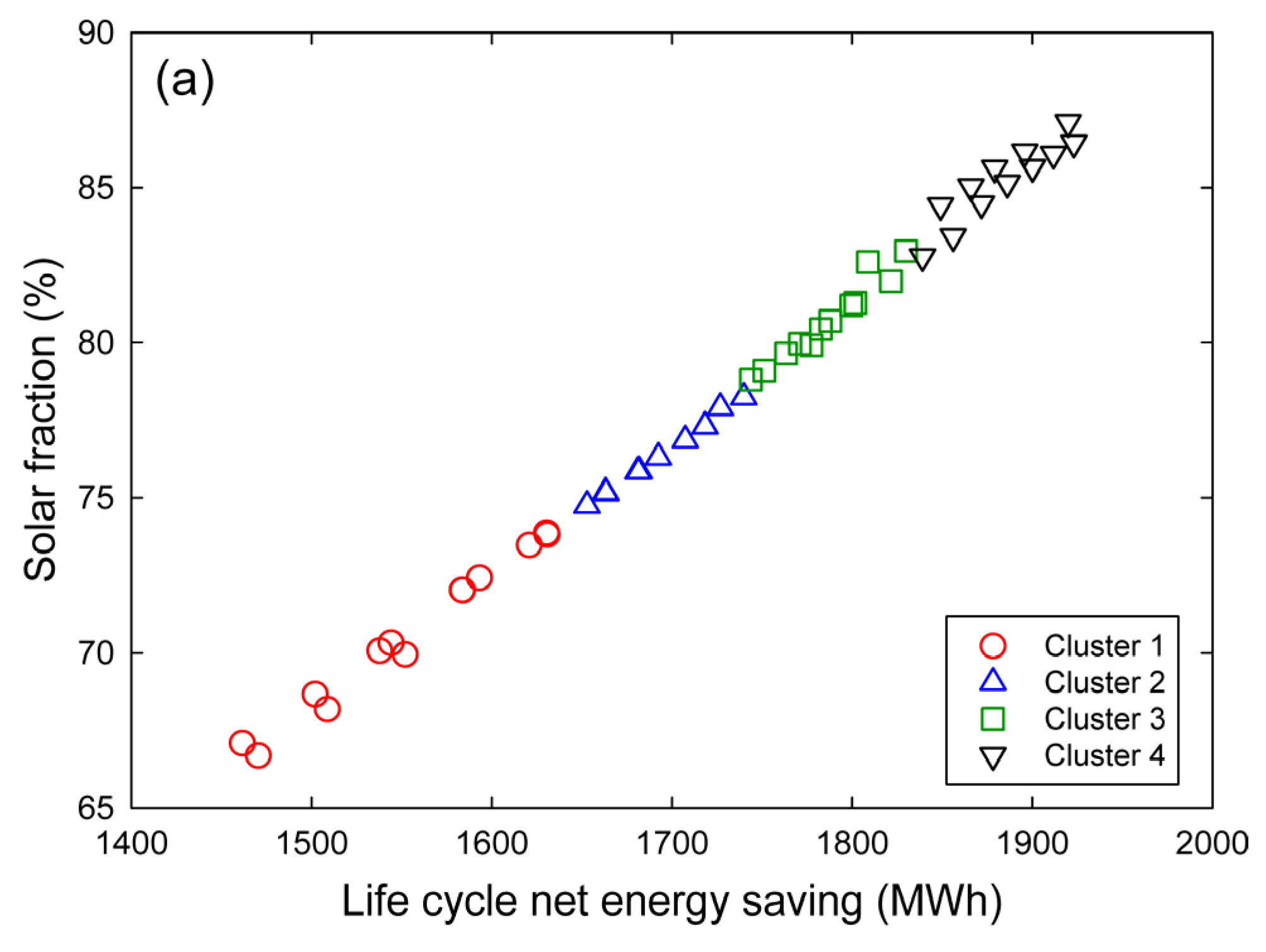
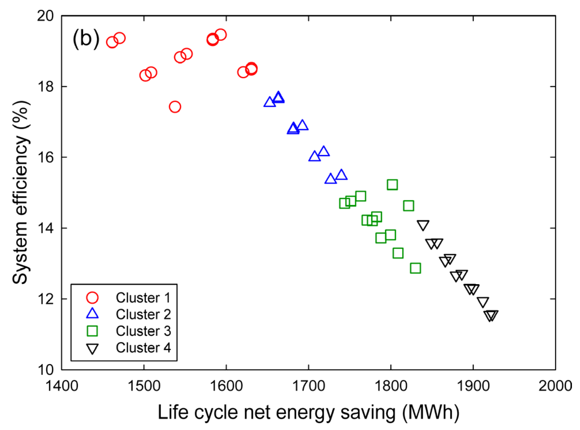
| Cluster 1 | Cluster 2 | Cluster 3 | Cluster 4 | |
| (-) | 4 | 4 | 4 | 4 |
| (ea.) | 73–85 | 91–109 | 115–139 | 127–163 |
| (m2) | 144.54–168.30 | 180.18–215.82 | 227.70–275.22 | 251.46–322.74 |
| (-) | 1–2 | 2 | 2–5 | 3–5 |
| (W/°C) | 3489–4071 | 4071 | 4071–5815 | 4652–5815 |
| (-) | 2–6 | 5–6 | 5–7 | 7 |
| (m3) | 3.76–6.92 | 6.21–6.92 | 6.21–9.58 | 9.58 |
| (-) | 4 | 4 | 4 | 4 |
| (ea.) | 1 | 1 | 1 | 1 |
| (kW) | 34.89 | 34.89 | 34.89 | 34.89 |
| (°) | 35–37 | 37–39 | 38–42 | 41–43 |
| (kg/s·m2) | 0.011–0.014 | 0.010–0.011 | 0.009–0.010 | 0.008–0.011 |
| (kg/s) | 0.604–0.707 | 0.686–0.746 | 0.712–0.910 | 0.791–1.029 |
| (%) | 66.7–73.9 | 74.8–78.2 | 78.8–83.0 | 82.8–87.1 |
| (%) | 17.4–19.5 | 15.4–17.7 | 12.9–15.2 | 11.5–14.1 |
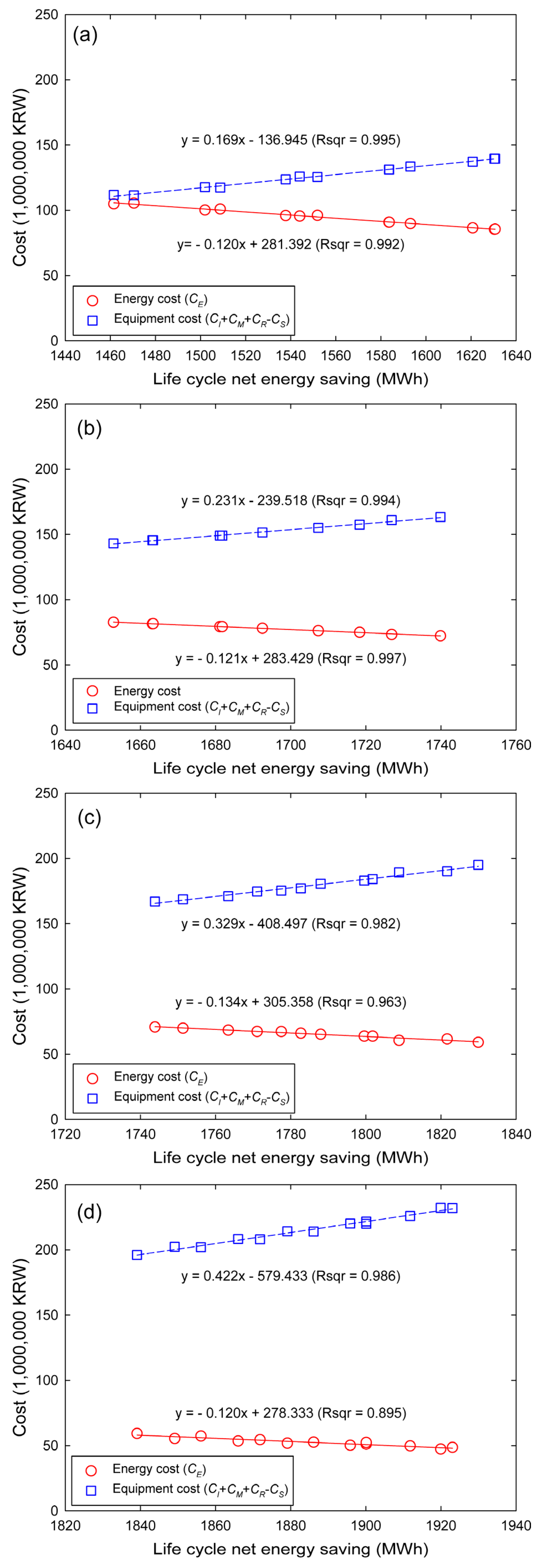
| (million KRW) | 85.4–105.5 | 72.3–82.7 | 59.1–70.8 | 47.4–59.3 |
| (million KRW) | 111.5–139.5 | 143.1–163.4 | 166.9–195.0 | 196.0–232.1 |
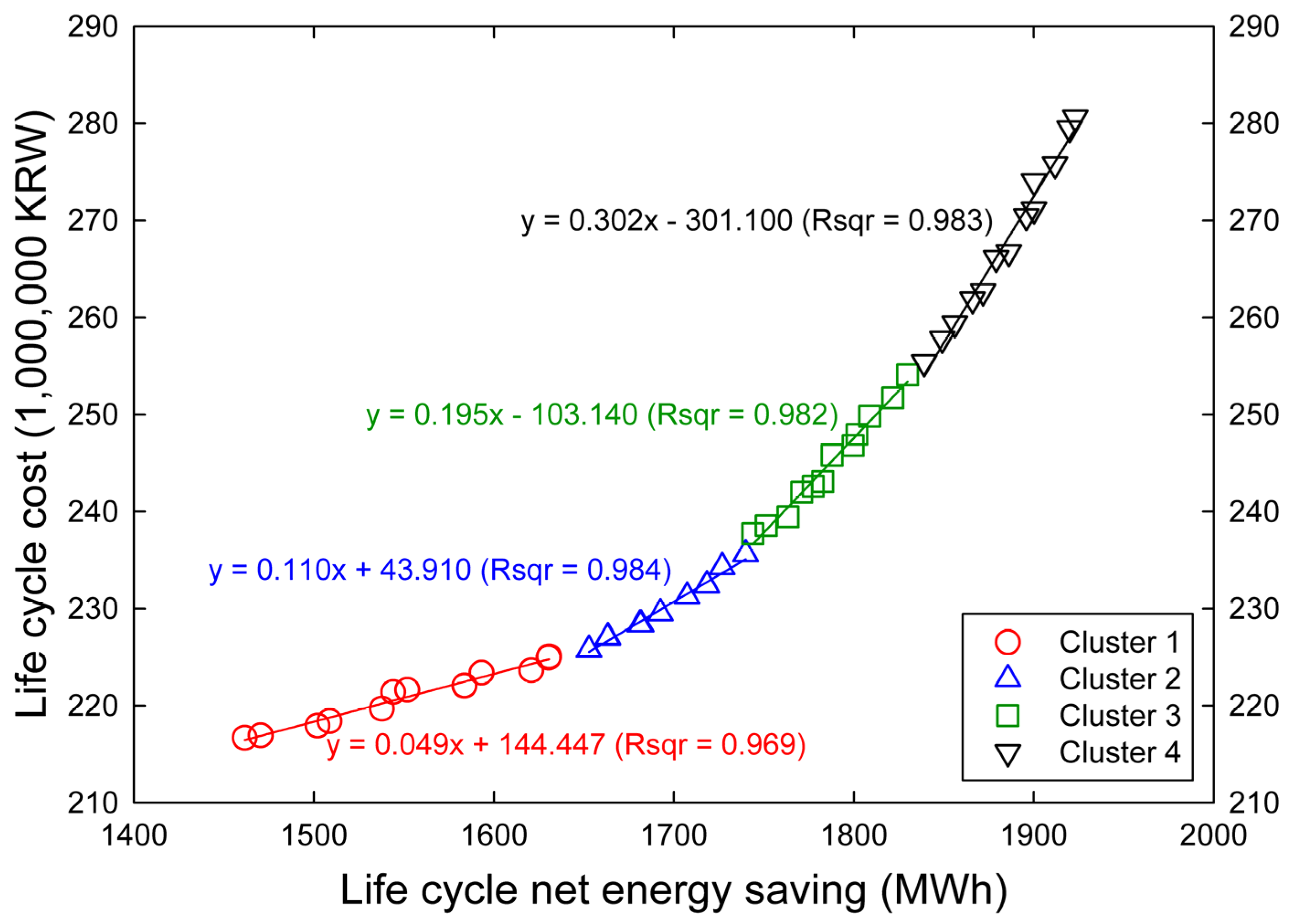
| (million KRW) | 216.7–225.1 | 225.8–235.6 | 237.7–254.1 | 255.4–280.6 |
| (MWh) | 1461.5–1630.7 | 1652.8–1739.9 | 1743.9–1829.9 | 1839.1–1923.1 |
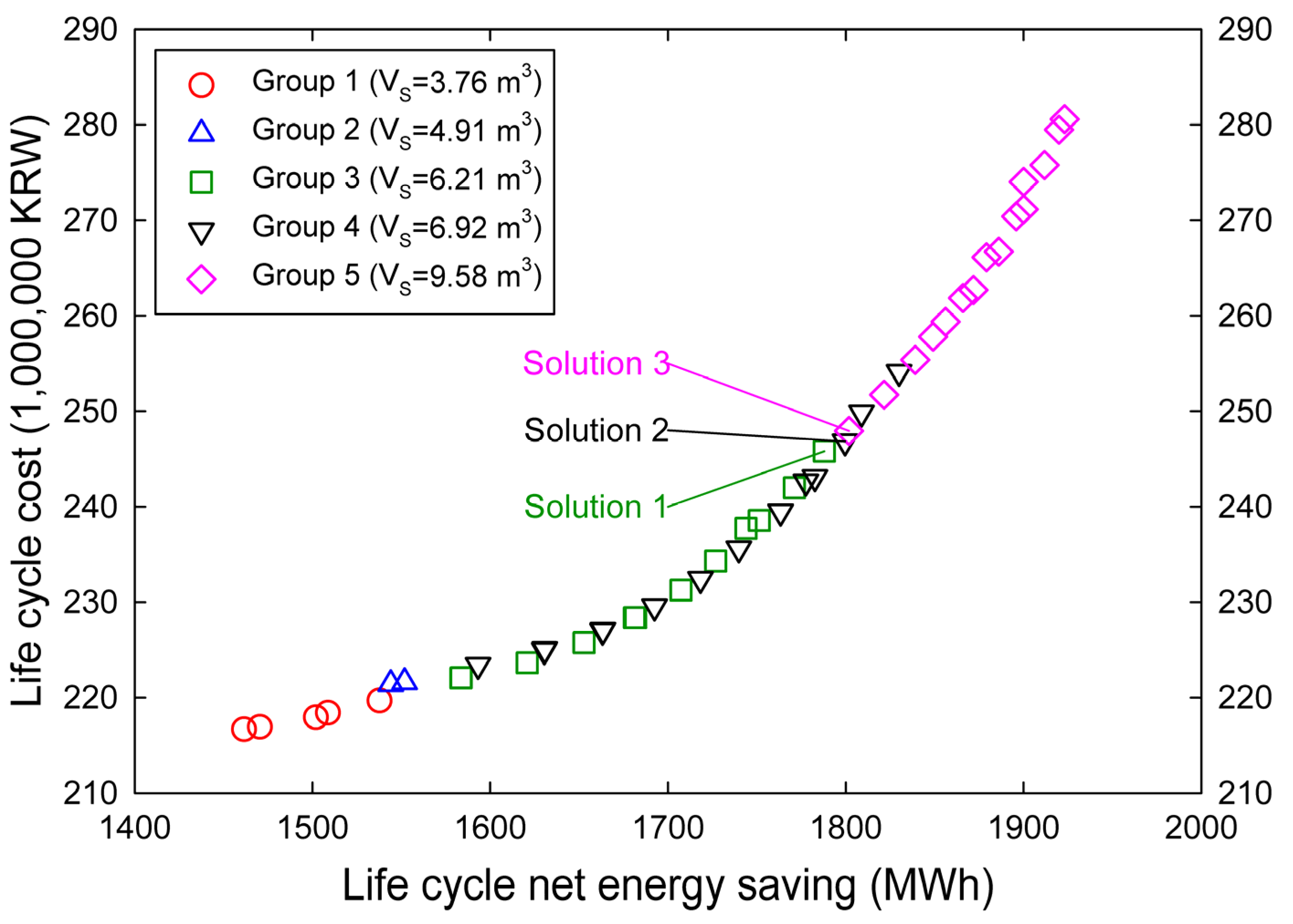
4.3. Characteristics of Non-Dominated Solutions according to RVA


| Parameter | Classification | ||
|---|---|---|---|
| Solution 1 | Solution 2 | Solution 3 | |
| (-) | 4 | 4 | 4 |
| (ea.) | 127 | 127 | 115 |
| (m2) | 251.46 | 251.46 | 227.70 |
| (-) | 3 | 3 | 3 |
| (W/°C) | 4652 | 4652 | 4652 |
| (-) | 5 | 6 | 7 |
| (m3) | 6.21 | 6.92 | 9.58 |
| (-) | 4 | 4 | 4 |
| (ea.) | 1 | 1 | 1 |
| (kW) | 34.89 | 34.89 | 34.89 |
| (°) | 41 | 41 | 40 |
| (kg/s·m2) | 0.009 | 0.009 | 0.010 |
| (kg/s) | 0.791 | 0.791 | 0.775 |
| (liter/m2) | 24.70 | 27.52 | 42.07 |
| (%) | 80.7 | 81.2 | 81.3 |
| (%) | 13.7 | 13.8 | 15.2 |
| (million KRW) | 65.23 | 63.84 | 63.81 |
| (million KRW) | 180.58 | 182.98 | 184.13 |
| (million KRW) | 245.81 | 246.82 | 247.94 |
| (MWh) | 1787.98 | 1799.58 | 1801.82 |
5. Conclusions
Acknowledgments
Conflicts of Interest
Nomenclature
| gross area of a single collector module, m2 | |
| gross area of the jth device of solar collectors, m2 | |
| area available to install solar collectors, m2 | |
| maximum capacity available to receive the subsidy cost, m2 | |
| surface area of a storage tank, m2 | |
| capacity rate of fluid on cold side of a heat exchanger, W/°C | |
| capacity rate of fluid on hot side of a heat exchanger, W/°C | |
| maximum capacity rate, W/°C | |
| minimum capacity rate, W/°C | |
| specific heat of water, J/kg·°C | |
| specific heat of collector fluid, J/kg·°C | |
| purchase cost of the jth auxiliary heater, KRW | |
| purchase cost of the jth solar collector, KRW | |
| purchase cost of the jth heat exchanger, KRW | |
| purchase cost of the jth storage tank, KRW | |
| energy cost, KRW | |
| initial cost, KRW | |
| initial cost of each component, KRW | |
| maintenance cost, KRW | |
| replacement cost, KRW | |
| replacement cost of each component, KRW | |
| subsidy cost, KRW | |
| life cycle cost, KRW | |
| hourly electricity cost, KRW/kWh | |
| hourly liquid natural gas (LNG) cost, KRW/m3 | |
| capacity rate ratio of a heat exchanger | |
| fuel price escalation rate, % | |
| energy input ratio of the auxiliary heaters | |
| hourly electricity consumption of the circulation pump, kWh | |
| hourly LNG consumption of the auxiliary heaters, m3 | |
| intercept of the efficiency curve of identical collector modules connected in series | |
| intercept of the efficiency curve of a single collector | |
| slope of the efficiency curve of identical collector modules connected in series, W/m2·°C | |
| slope of the efficiency curve of a single collector, W/m2·°C | |
| solar fraction of the solar system over a given time horizon, % | |
| acceleration due to gravity, m/s2 | |
| height of the jth device of solar collectors, m | |
| circulation pump head, m | |
| global solar radiation on a horizontal surface, W/m2 | |
| hourly beam solar radiation on a horizontal surface, W/m2 | |
| hourly diffuse solar radiation on a horizontal surface, W/m2 | |
| hourly total solar radiation on the tilted collector array, W/m2 | |
| real discount rate, % | |
| mass flow rate per unit area of the collector fluid, kg/s·m2 | |
| mass flow rate on the cold side of the heat exchanger, kg/s | |
| mass flow rate of the discharged water from a storage tank, kg/s | |
| mass flow rate of the fluid passing through the pump, kg/s | |
| mass flow rate from the storage tank to the load, kg/s | |
| mass flow rate of the desired hot water load, kg/s | |
| number of parallel connections in the collector array | |
| number of identical collectors in series | |
| maximum number of identical collectors in series | |
| number of the jth devices of solar collectors | |
| number of the jth devices of auxiliary heaters | |
| number of exchanger heat transfer units | |
| planning period, year | |
| life span of each component, year | |
| Number of times each component is replaced | |
| primary energy factor for electricity | |
| part load ratio of the auxiliary heaters at each time step | |
| heating capacity of the jth device of auxiliary heaters, kW | |
| total heating capacity of the auxiliary heaters, kW | |
| hourly hot water load, Wh | |
| life cycle net energy cost of the solar system over the planning period, MWh | |
| peak hot water load, kW | |
| lower heating value of LNG, m3/W | |
| auxiliary heating energy, W | |
| discharged heat to avoid overheating of a storage tank, W | |
| heat loss of a storage tank, W | |
| solar energy extracted from the storage tank to the load, W | |
| solar energy supplied to a storage tank, W | |
| solar useful heat gain of identical collectors in series, W | |
| the ratio of the beam radiation on the tilted surface to that on a horizontal surface | |
| percentage of the supplementary cost against the direct purchase cost, % | |
| percentage of the annual maintenance cost against the initial cost, % | |
| percentage of subsidy cost against the initial cost, % | |
| outdoor dry-bulb temperature, °C | |
| ambient temperature, °C | |
| cold stream inlet temperature of a heat exchanger, °C | |
| cold stream outlet temperature of a heat exchanger, °C | |
| upper input temperature of the differential temperature controller (DTC), °C | |
| hot stream inlet temperature of a heat exchanger, °C | |
| hot stream outlet temperature of a heat exchanger, °C | |
| lower input temperature of the DTC, °C | |
| desired hot water temperature, °C | |
| make-up water temperature, °C | |
| storage tank temperature at the beginning of the time step, °C | |
| storage tank temperature at the end of the time step, °C | |
| maximum allowable storage tank temperature, °C | |
| type of auxiliary heater | |
| type of solar collector | |
| type of heat exchanger | |
| type of storage tank | |
| heat loss coefficient of a storage tank, W/m2·°C | |
| product of the overall heat transfer coefficient and area of a heat exchanger, W/°C | |
| uniform present value factor adjusted to reflect the electricity price escalation rate | |
| uniform present value factor adjusted to reflect the LNG price escalation rate | |
| uniform present value factor adjusted to reflect the fuel price escalation rate | |
| storage tank volume, m3 | |
| width of the jth device of solar collectors, m | |
| meridian altitude in winter, ° | |
| slope of the collector array, ° | |
| output control function of the DTC | |
| effectiveness of a heat exchanger | |
| overall efficiency of auxiliary heater | |
| motor efficiency of circulation pump | |
| pumping efficiency of circulation pump | |
| efficiency of the solar system over a given time horizon | |
| ground reflectance | |
| density of water, kg/m3 | |
| upper deadband temperature difference of the DTC, °C | |
| lower deadband temperature difference of the DTC, °C |
Appendix
| Parameters | Types | ||||
|---|---|---|---|---|---|
| 0 | 1 | 2 | 3 | 4 | |
| Interceptofcollectorefficiency (-) | 0.7445 | 0.7208 | 0.7200 | 0.7109 | 0.7043 |
| Negative ofslopeofcollectorefficiency (W/m2·°C) | 4.8483 | 4.7999 | 4.0900 | 5.0050 | 4.5368 |
| Flow rate of fluid understandardconditions (kg/s) | 0.0381 | 0.0373 | 0.0400 | 0.0368 | 0.0368 |
| Overall height (m) | 2.00 | 2.00 | 2.00 | 2.02 | 2.00 |
| Overall width (m) | 1.00 | 1.00 | 1.00 | 1.00 | 0.99 |
| Life span (year) | 20 | 20 | 20 | 20 | 20 |
| Purchasecost (1000 KRW/ea.) | 545 | 530 | 520 | 545 | 540 |
| Parameters | Types | |||||||
|---|---|---|---|---|---|---|---|---|
| 0 | 1 | 2 | 3 | 4 | 5 | 6 | 7 | |
| Overall heat transfer coefficient-area product (W/°C) | 2908 | 3489 | 4071 | 4652 | 5234 | 5815 | 6978 | 8141 |
| Total heat transfer area (m2) | 0.8398 | 1.0608 | 1.2376 | 1.4000 | 1.5400 | 1.6800 | 2.1000 | 2.3800 |
| Area per plate (m2) | 0.0442 | 0.0442 | 0.0442 | 0.1400 | 0.1400 | 0.1400 | 0.1400 | 0.1400 |
| Total number of plates | 21 | 26 | 30 | 12 | 13 | 14 | 17 | 19 |
| Life span (year) | 5 | 5 | 5 | 5 | 5 | 5 | 5 | 5 |
| Purchase cost (1000 KRW/ea.) | 670 | 730 | 780 | 1050 | 1070 | 1100 | 1170 | 1220 |
| Parameters | Types | |||||||
|---|---|---|---|---|---|---|---|---|
| 0 | 1 | 2 | 3 | 4 | 5 | 6 | 7 | |
| Tank volume (m3) | 1.72 | 2.65 | 3.76 | 4.91 | 5.54 | 6.21 | 6.92 | 9.58 |
| Heatlosscoefficient (W/°C) | 0.3 | 0.3 | 0.3 | 0.3 | 0.3 | 0.3 | 0.3 | 0.3 |
| Overall height (m) | 1.52 | 2.00 | 2.44 | 2.44 | 2.44 | 2.44 | 3.05 | 3.05 |
| Overall diameter (m) | 1.20 | 1.30 | 1.40 | 1.60 | 1.70 | 1.80 | 1.70 | 2.00 |
| Life span (year) | 15 | 15 | 15 | 15 | 15 | 15 | 15 | 15 |
| Purchasecost (1,000,000 KRW/ea.) | 9.49 | 10.73 | 12.65 | 15.88 | 17.33 | 18.02 | 18.98 | 24.00 |
| Parameters | Types | |||||
|---|---|---|---|---|---|---|
| 0 | 1 | 2 | 3 | 4 | 5 | |
| Rated heating capacity (kW) | 15.12 | 18.61 | 23.26 | 29.08 | 34.89 | 58.15 |
| Rated efficiency (%) | 83 | 84 | 85 | 86 | 86 | 82 |
| Life span (year) | 15 | 15 | 15 | 15 | 15 | 15 |
| Purchase cost (1000 KRW/ea.) | 807 | 844 | 909 | 964 | 1039 | 2291 |
References
- Hottel, H.C.; Whillier, A. Evaluation of Flat-Plate Collector Performance; University of Arizona Press: Tucson, AZ, USA, 1958. [Google Scholar]
- Klein, S.A. Calculation of flat-plate collector utilizability. Sol. Energy 1978, 21, 393–402. [Google Scholar] [CrossRef]
- Klein, S.A.; Beckman, W.A.; Duffie, J.A. A design procedure for solar heating systems. Sol. Energy 1976, 18, 113–127. [Google Scholar] [CrossRef]
- Klein, S.A.; Beckman, W.A. A general design method for closed-loop solar energy systems. Sol. Energy 1979, 22, 269–282. [Google Scholar] [CrossRef]
- Klein, S.A.; Cooper, P.I.; Freeman, T.L.; Beekman, D.L.; Beckman, W.A.; Duffie, J.A. A method of simulation of solar processes and its application. Sol. Energy 1975, 17, 29–37. [Google Scholar] [CrossRef]
- Lund, P.D.; Peltola, S.S. SOLCHIPS—A fast predesign and optimization tool for solar heating with seasonal storage. Sol. Energy 1992, 48, 291–300. [Google Scholar] [CrossRef]
- Atia, D.M.; Fahmy, F.H.; Ahmed, N.M.; Dorrah, H.T. Optimal sizing of a solar water heating system based on a genetic algorithm for an aquaculture system. Math. Comput. Model 2012, 55, 1436–1449. [Google Scholar] [CrossRef]
- Matrawy, K.K.; Farkas, I. New technique for short term storage sizing. Renew. Energy 1997, 11, 129–141. [Google Scholar] [CrossRef]
- Michelson, E. Multivariate optimization of a solar water heating system using the Simplex method. Sol. Energy 1982, 29, 89–99. [Google Scholar] [CrossRef]
- Loomans, M.; Visser, H. Application of the genetic algorithm for optimization of large solar hot water systems. Sol. Energy 2002, 72, 427–439. [Google Scholar] [CrossRef]
- Krause, M.; Vajen, K.; Wiese, F.; Ackermann, H. Investigation on optimizing large solar thermal systems. Sol. Energy 2002, 73, 217–225. [Google Scholar] [CrossRef]
- Kalogirou, S.A. Optimization of solar systems using artificial neural-networks and genetic algorithms. Appl. Energy 2004, 77, 383–405. [Google Scholar] [CrossRef]
- Kim, Y.D.; Thu, K.; Bhatia, H.K.; Bhatia, C.S.; Ng, K.C. Thermal analysis and performance optimization of a solar hot water plant with economic evaluation. Sol. Energy 2012, 86, 1378–1395. [Google Scholar] [CrossRef]
- Ko, M.J. Analysis and optimization design of a solar water heating system based on life cycle cost using a genetic algorithm. Energies 2015, 8, 11380–11403. [Google Scholar] [CrossRef]
- Ko, M.J. A novel design method for optimizing an indirect forced circulation solar water heating system based on life cycle cost using a genetic algorithm. Energies 2015, 8, 11592–11617. [Google Scholar] [CrossRef]
- Bornatico, R.; Pfeiffer, M.; Witzig, A.; Guzzella, L. Optimal sizing of a solar thermal building installation using particle swarm optimization. Energy 2012, 41, 31–37. [Google Scholar] [CrossRef]
- Sadafi, M.H.; Hosseini, R.; Safikhani, H.; Bagheri, A.; Mahmoodabadi, M.J. Multi-objective optimization of solar thermal energy storage using hybrid of particle swarm optimization, multiple crossover and mutation operator. Int. J. Eng. Trans. B 2011, 24, 367–376. [Google Scholar] [CrossRef]
- Cheng Hin, J.N.; Zmeureanu, R. Optimization of a residential solar combisystem for minimum life cycle cost, energy use and exergy destroyed. Sol. Energy 2014, 100, 102–113. [Google Scholar] [CrossRef]
- Kusyy, O.; Kuethe, S.; Vajen, K. Simulation-based optimization of a solar water heating system by a hybrid genetic-binary search algorithm. In Proceedings of the 2010 Xvth International Seminar/Workshop on Direct and Inverse Problems of Electromagnetic and Acoustic Wave Theory (DIPED), Tbilisi, GA, USA, 27–30 September 2010; IEEE: Piscataway, NJ, USA.
- Shariah, A.M.; Löf, G.O.G. The optimization of tank-volume-to-collector-area ratio for a thermosyphon solar water heater. Renew. Energy 1996, 7, 289–300. [Google Scholar] [CrossRef]
- Hobbi, A.; Siddiqui, K. Optimal design of a forced circulation solar water heating system for a residential unit in cold climate using TRNSYS. Sol. Energy 2009, 83, 700–714. [Google Scholar] [CrossRef]
- Yan, C.; Wang, S.; Ma, Z.; Shi, W. A simplified method for optimal design of solar water heating systems based on life-cycle energy analysis. Renew. Energy 2015, 74, 271–278. [Google Scholar] [CrossRef]
- Lima, J.B.A.; Prado, R.T.A.; Taborianski, V.M. Optimization of tank and flat-plate collector of solar water heating system for single-family households to assure economic efficiency through the TRNSYS program. Renew. Energy 2006, 31, 1581–1595. [Google Scholar] [CrossRef]
- Choi, D.S.; Ko, M.J. Optimization design for a solar water heating system using the genetic algorithm. Int. J. Appl. Eng. Res. 2015, 10, 27031–27042. [Google Scholar]
- Kulkarni, G.N.; Kedare, S.B.; Bandyopadhyay, S. Determination of design space and optimization of solar water heating systems. Sol. Energy 2007, 81, 958–968. [Google Scholar] [CrossRef]
- Kulkarni, G.N.; Kedare, S.B.; Bandyopadhyay, S. Optimization of solar water heating systems through water replenishment. Energy Convers. Manag. 2009, 50, 837–846. [Google Scholar] [CrossRef]
- Deb, K. Multi-Objective Optimization Using Evolutionary Algorithms; Wiley: Chichester, UK, 2009. [Google Scholar]
- Konak, A.; Coit, D.W.; Smith, A.E. Multi-objective optimization using genetic algorithms: A tutorial. Reliab. Eng. Syst. Saf. 2006, 91, 992–1007. [Google Scholar] [CrossRef]
- Li, Y.; Liao, S.; Liu, G. Thermo-economic multi-objective optimization for a solar-dish Brayton system using NSGA-II and decision making. Int. J. Electr. Power Energy Syst. 2015, 64, 167–175. [Google Scholar] [CrossRef]
- Ahmadi, M.H.; Dehghani, S.; Mohammadi, A.H.; Feidt, M.; Barranco-Jimenez, M.A. Optimal design of a solar driven heat engine based on thermal and thermo-economic criteria. Energy Convers. Manag. 2013, 75, 635–642. [Google Scholar] [CrossRef]
- Khorasaninejad, E.; Hajabdollahi, H. Thermo-economic and environmental optimization of solar assisted heat pump by using multi-objective particle swarm algorithm. Energy 2014, 72, 680–690. [Google Scholar] [CrossRef]
- Gebreslassie, B.H.; Jimenez, M.; Guillén-Gosálbez, G.; Jiménez, L.; Boer, D. Multi-objective optimization of solar assisted absorption cooling system. Comput. Aided Chem. Eng. 2010, 28, 1033–1038. [Google Scholar]
- Gebreslassie, B.H.; Guillén-Gosálbez, G.; Jiménez, L.; Boer, D. Solar assisted absorption cooling cycles for reduction of global warming: A multi-objective optimization approach. Sol. Energy 2012, 86, 2083–2094. [Google Scholar] [CrossRef]
- Wang, M.; Wang, J.; Zhao, P.; Dai, Y. Multi-objective optimization of a combined cooling, heating and power system driven by solar energy. Energy Convers. Manag. 2015, 89, 289–297. [Google Scholar] [CrossRef]
- Hang, Y.; Du, L.; Qu, M.; Peeta, S. Multi-objective optimization of integrated solar absorption cooling and heating systems for medium-sized office buildings. Renew. Energy 2013, 52, 67–78. [Google Scholar] [CrossRef]
- Boyaghchi, F.A.; Heidarnejad, P. Thermoeconomic assessment and multi objective optimization of a solar micro CCHP based on Organic Rankine Cycle for domestic application. Energy Convers. Manag. 2015, 97, 224–234. [Google Scholar] [CrossRef]
- Duffie, J.A.; Beckman, W.A. Solar Engineering of Thermal Processes, 3rd ed.; Wiley: Hoboken, NJ, USA, 2006. [Google Scholar]
- Henderson, H.; Huang, Y.J.; Parker, D. Residential Equipment Part Load Curve for Use in DOE-2: Technical Report LBNL-42175; Lawrence Berkeley National Laboratory: Berkeley, CA, USA, 1999. [Google Scholar]
- Deb, K.; Pratap, A.; Agarwal, S.; Meyarivan, T. A fast and elitist multiobjective genetic algorithm: NSGA-II. IEEE Trans. Evol. Comput. 2002, 6, 182–197. [Google Scholar] [CrossRef]
- Kanpur Genetic Algorithms Laboratory. Available online: http://www.iitk.ac.in/kangal/codes.shtml (accessed on 29 January 2015).
- National Renewable Energy Laboratory. Available online: http://www.nrel.gov/docs/fy11osti/46861.pdf (accessed on 29 January 2015).
- Korea Law. Available online: http://www.law.go.kr (accessed on 16 October 2015).
- Beckman, W.A.; Klein, S.A.; Duffie, J.A. Solar Heating Design by the F-Chart Method; John Wiley: New York, NY, USA, 1977. [Google Scholar]
- Baughn, J.W.; Young, M.F. The calculated performance of a solar hot water system for a range of collector flow rates. Sol. Energy 1984, 32, 303–305. [Google Scholar] [CrossRef]
- Lund, P.D.; Keinonen, R.S. Economic analysis of central solar heating systems with seasonal storage: Report TKK-F-A589; Helsinki University of Technology: Espoo, Finland, 1985. [Google Scholar]
© 2015 by the authors; licensee MDPI, Basel, Switzerland. This article is an open access article distributed under the terms and conditions of the Creative Commons by Attribution (CC-BY) license (http://creativecommons.org/licenses/by/4.0/).
Share and Cite
Ko, M.J. Multi-Objective Optimization Design for Indirect Forced-Circulation Solar Water Heating System Using NSGA-II. Energies 2015, 8, 13137-13161. https://doi.org/10.3390/en81112360
Ko MJ. Multi-Objective Optimization Design for Indirect Forced-Circulation Solar Water Heating System Using NSGA-II. Energies. 2015; 8(11):13137-13161. https://doi.org/10.3390/en81112360
Chicago/Turabian StyleKo, Myeong Jin. 2015. "Multi-Objective Optimization Design for Indirect Forced-Circulation Solar Water Heating System Using NSGA-II" Energies 8, no. 11: 13137-13161. https://doi.org/10.3390/en81112360