
Adaptive Neuro-Fuzzy Inference Systems as a Strategy for Predicting and Controling the Energy Produced from Renewable Sources


Abstract
:1. Introduction
2. Exploration and Assessment of Criteria Used for Choosing a Forecasting Tool
2.1. Data Preprocessing
- –
- : Scaled Value;
- –
- : maximum value of data;
- –
- : minimum value of data;
- –
- : maximum of transformation;
- –
- : minimum of transformation;
- –
- : Original Value.
2.2. Determining NN Architecture
2.3. Parametrization
2.4. Implementation and Performance Testing

| Commonly Used Forecast Accuracy Measures | ||
|---|---|---|
| MSE | Mean Squared Error | =mean() |
| RMSE | Root Mean Squared Error | = |
| MAE | Mean Absolute Error | =mean() |
| MdAE | Median Absolute Error | =median() |
| MAPE | Mean Absolute Percentage Error | =mean() |
| MdAPE | Median Absolute Percentage Error | =median() |
| MRAE | Mean Relative Absolute Error | =mean() |
| MdRAE | Median Relative Absolute Error | =median() |
| GMRAE | Geometric Mean Relative Absolute Error | =gmean() |
| RelMAE | Relative Mean Absolute Error | =MAE/MAEb |
| RelRMSE | Relative Root Mean Squared Error | =RMSE/RMSEb |
| LMR | Log Mean squared error Ratio | =log(RelMSE) |
| PB | Percentage better | =100*mean() |
| PB (MAE) | Percentage better (MAE) | =100*mean() |
| PB(MSE) | Percentage better (MSE) | =100*mean() |
3. Forecasting Tool Simulation and Performance Evaluation
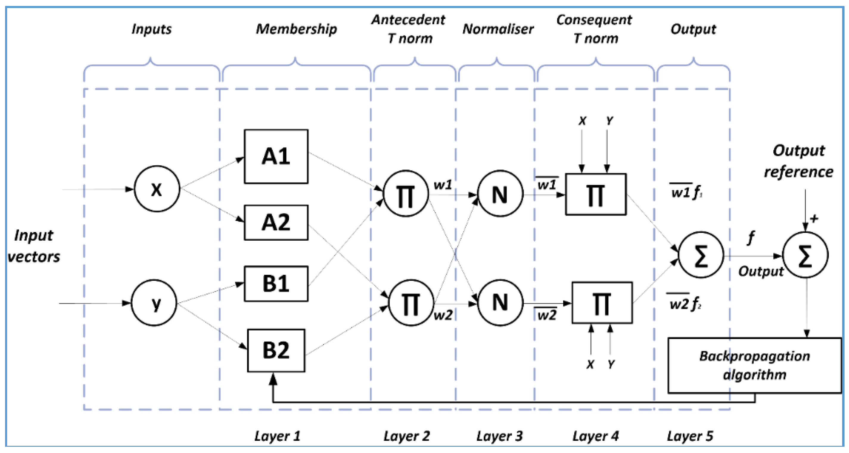
3.1. Adaptive Neuro-Fuzzy Inference System

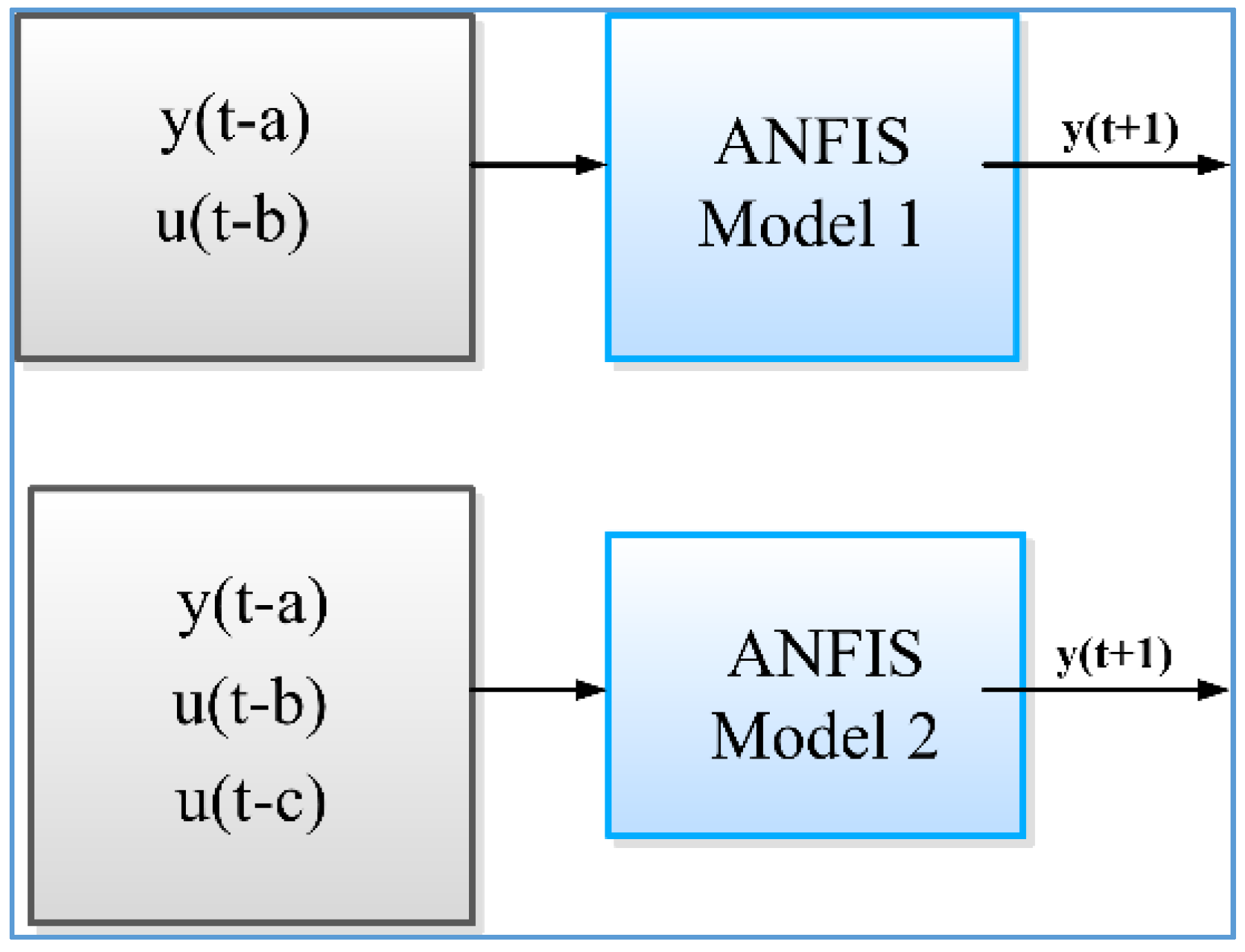
3.2. Simulation Conditions and Strategy
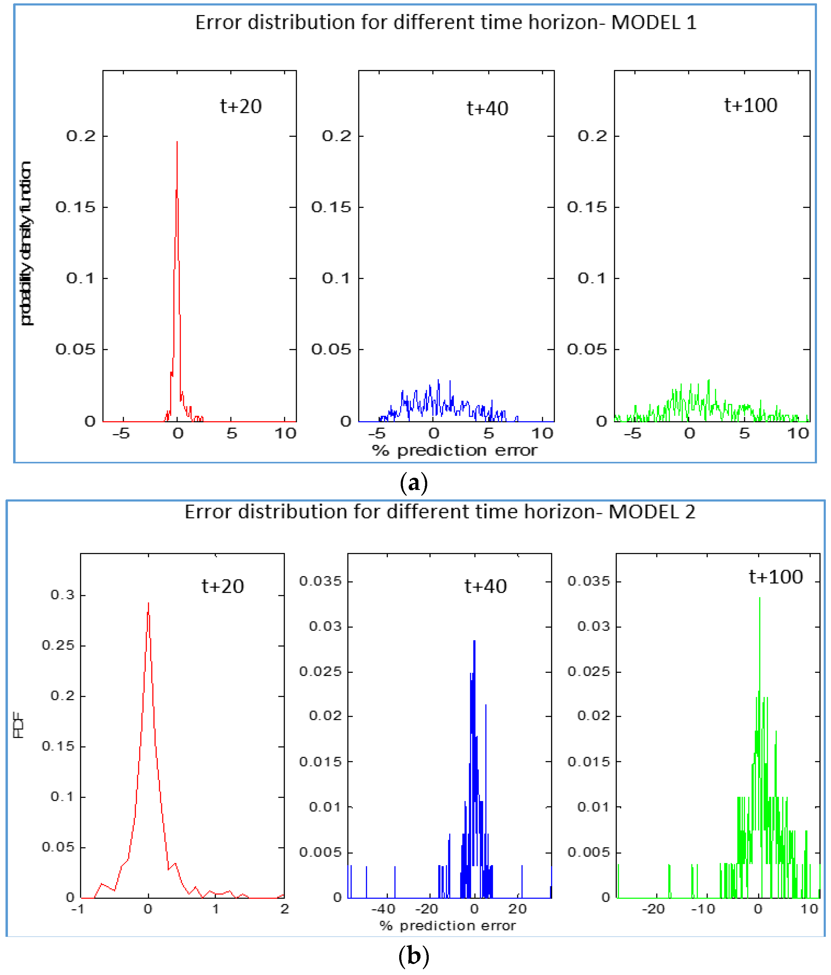
- Model 1 represents an ANFIS structure with two inputs {(y(t − a), u(t − b))}
- Model 2 is an ANFIS structure with three inputs: {(y(t − a), u(t − b), u(t − c))}, a = 1,...4; b, c = 1, ... 6

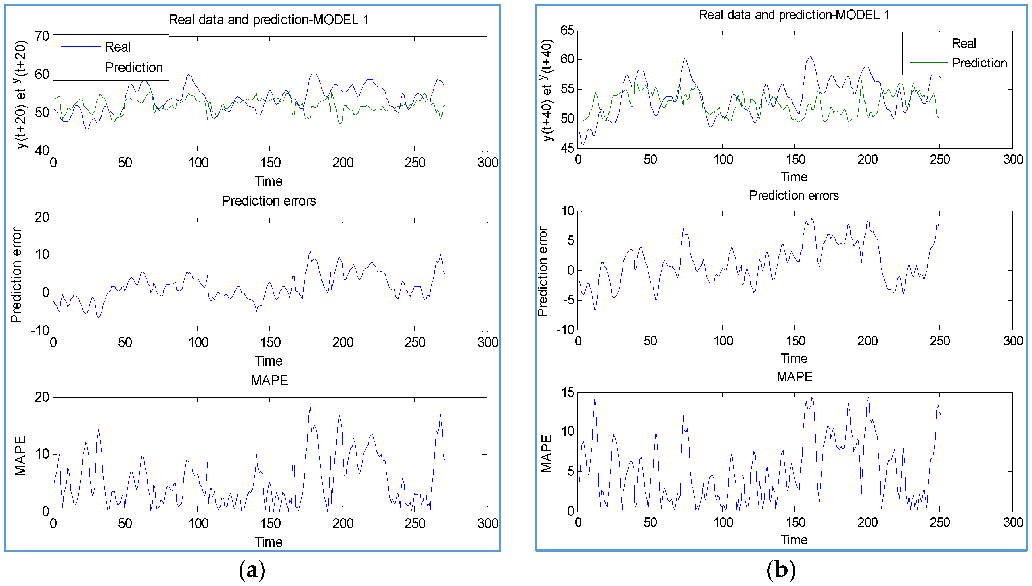
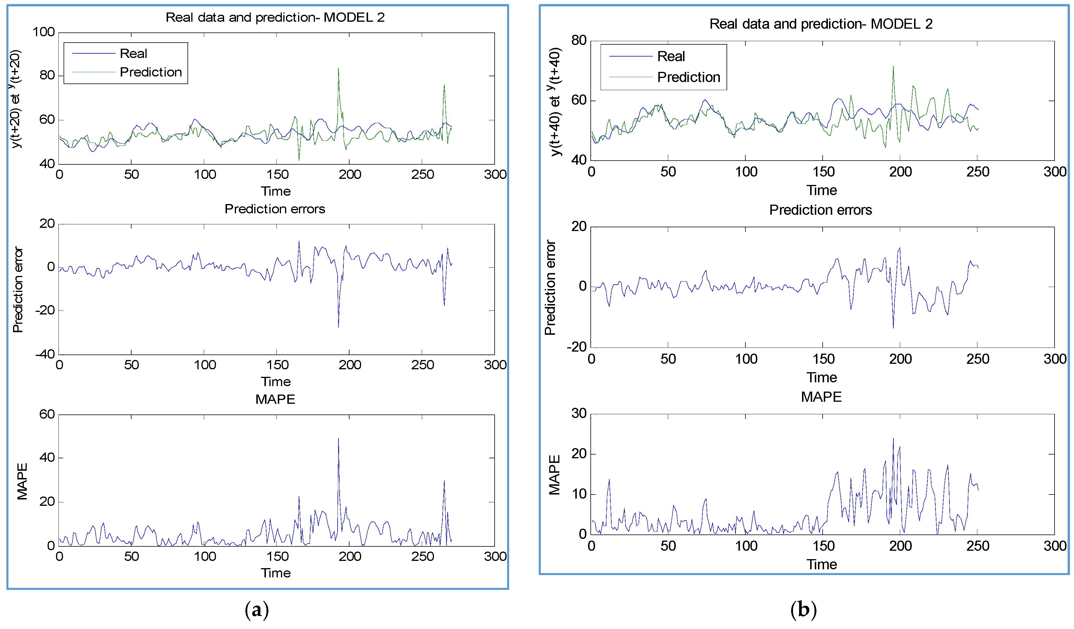
4. Simulations Results
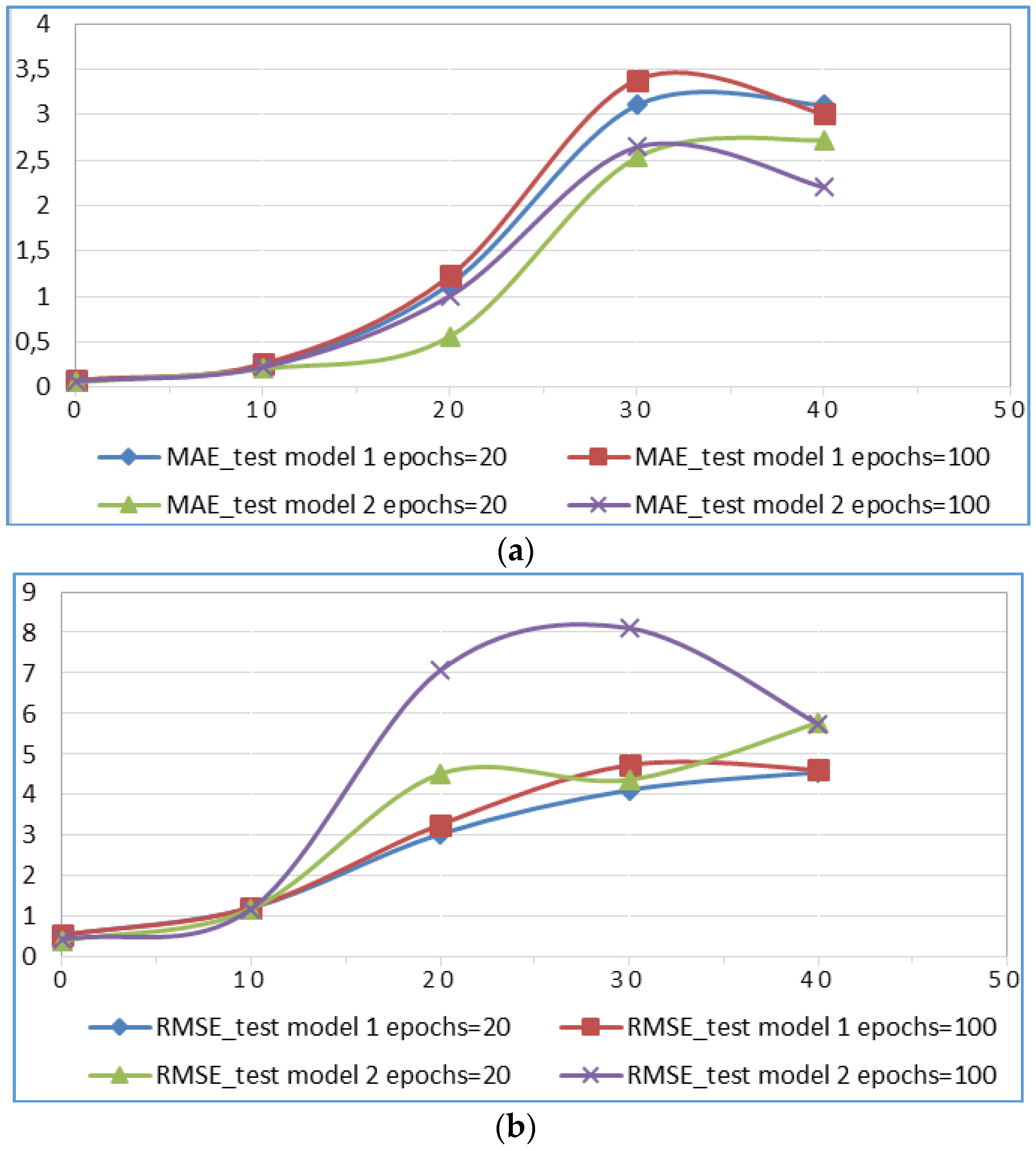
4.1. Scenario 1


| t + pred | ANFIS | RMSE_Test | MAE_Test | ||
|---|---|---|---|---|---|
| Epochs = 20 | Epochs = 100 | Epochs = 20 | Epochs = 100 | ||
| 1 | model 1 | 0,5532 | 0,5514 | 0,0809 | 0,0816 |
| 1 | model 2 | 0,4083 | 0,4432 | 0,0597 | 0,0708 |
| 4 | model 1 | 1,2228 | 1,23 | 0,2384 | 0,2591 |
| 4 | model 2 | 1,1955 | 1,1959 | 0,2042 | 0,2239 |
| 10 | model 1 | 3,0388 | 3,2713 | 1,1357 | 1,226 |
| 10 | model 2 | 4,5201 | 7,0661 | 0,5617 | 1,0066 |
| 20 | model 1 | 4,1209 | 4,7385 | 3,1039 | 3,382 |
| 20 | model 2 | 4,374 | 8,1093 | 2,5285 | 2,6426 |
| 40 | model 1 | 4,5597 | 4,622 | 3,1039 | 3,0073 |
| 40 | model 2 | 5,7804 | 5,7492 | 2,7198 | 2,2013 |
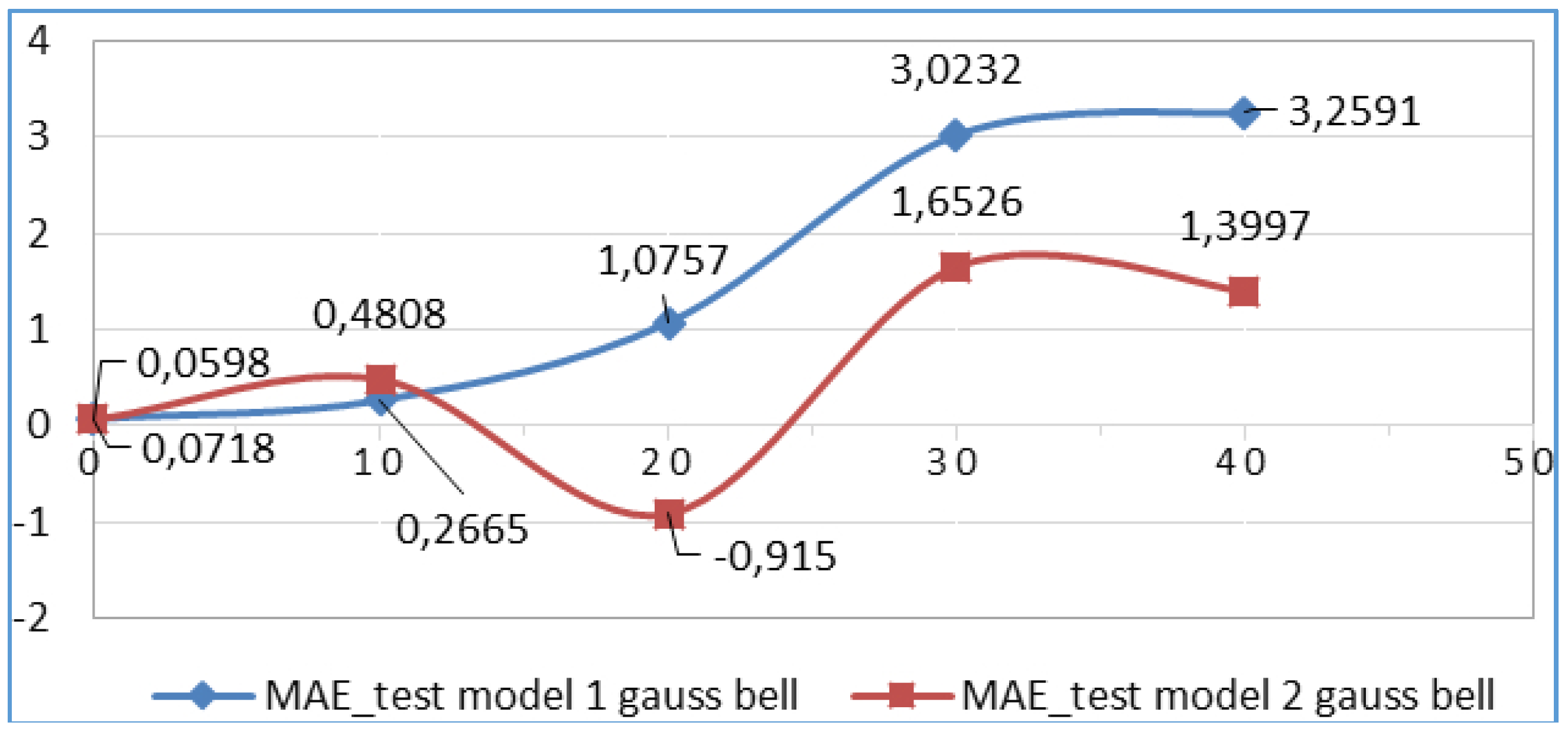
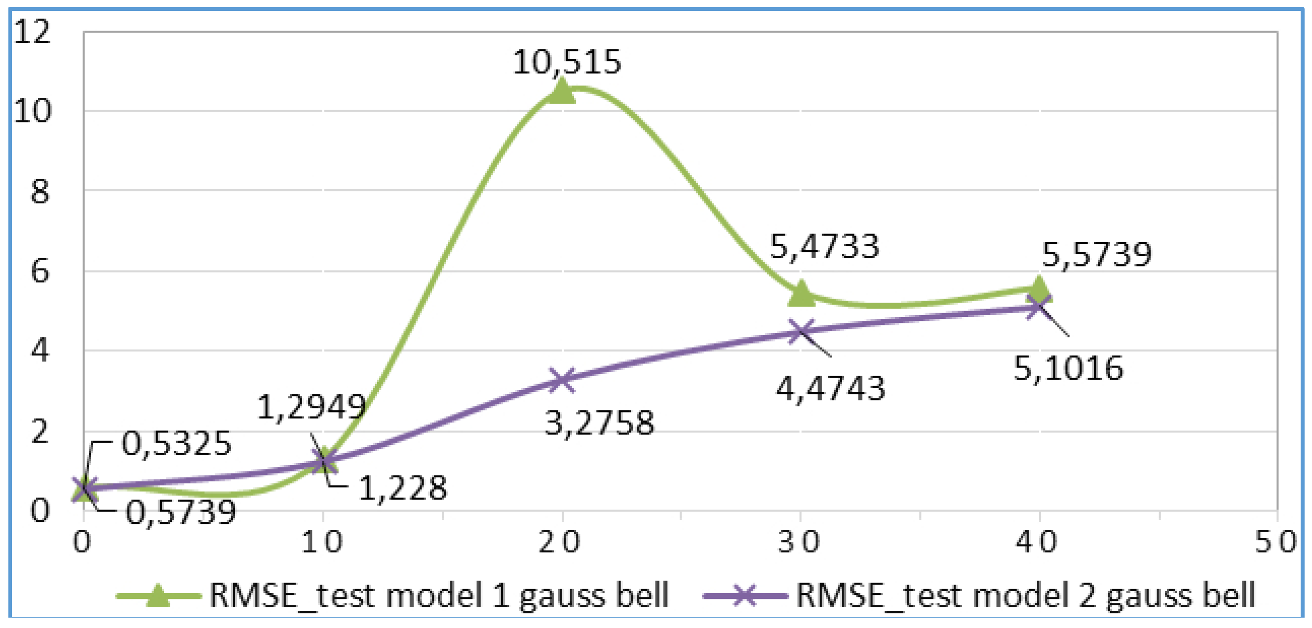
4.2. Scenario 2
| t + pred | ANFIS | MAE_Test | RMSE_Test | |||
|---|---|---|---|---|---|---|
| Type | No | Model 1 | Model 2 | Model 1 | Model 2 | |
| 1 | gbellmf | 2 | 0,0718 | 0,0579 | 0,4186 | 0,5325 |
| 4 | gbellmf | 2 | 0,2665 | 0,2863 | 1,1395 | 1,228 |
| 10 | gbellmf | 2 | 1,0757 | −915 | 10,515 | 3,2758 |
| 20 | gbellmf | 2 | 3,3012 | 1,6894 | 5,3083 | 4,8206 |
| 40 | gbellmf | 2 | 3,0616 | 1,3997 | 5,5443 | 4,7185 |
| 1 | gaussmf | 2 | 0,0718 | 0,0579 | 0,4186 | 0,5325 |
| 4 | gaussmf | 2 | 0,2665 | 0,2863 | 1,1395 | 1,228 |
| 10 | gaussmf | 2 | 1,0757 | −915 | 10,515 | 3,2758 |
| 20 | gaussmf | 2 | 3,3012 | 1,6894 | 5,3083 | 4,8206 |
| 40 | gaussmf | 2 | 3,0616 | 1,3997 | 5.5443 | 4,7185 |
| t + pred | ANFIS | MAE_Test | RMSE_Test | |||
|---|---|---|---|---|---|---|
| Type | No | Model 1 | Model 2 | Model 1 | Model 2 | |
| 1 | gbellmf | 3 | 0,0718 | 0,0598 | 0,5739 | 0,5325 |
| 4 | gbellmf | 3 | 0,2665 | 0,4808 | 1,2949 | 1,228 |
| 10 | gbellmf | 3 | 1,0757 | −0,915 | 10,515 | 3,2758 |
| 20 | gbellmf | 3 | 3,0232 | 1,6526 | 5,4733 | 4,4743 |
| 40 | gbellmf | 3 | 3,2591 | 1,3997 | 5,5739 | 5,1016 |
| 1 | gaussmf | 3 | 0,0718 | 0,0598 | 0,5739 | 0,5325 |
| 4 | gaussmf | 3 | 0,2665 | 0,4808 | 1,2949 | 1,228 |
| 10 | gaussmf | 3 | 1,0757 | −0,915 | 10,515 | 3,2758 |
| 20 | gaussmf | 3 | 3,0232 | 1,6526 | 5,4733 | 4,4743 |
| 40 | gaussmf | 3 | 3,2591 | 1,3997 | 5,5739 | 5,1016 |


5. Conclusions
Acknowledgments
Author Contributions
Conflicts of Interest
References
- Boyle, G. Renewable Energy: Power for a Sustainable Future; Oxford University Press: Oxford, UK, 2012. [Google Scholar]
- Sorensen, B. Renewable Energy, Fourth Edition: Physics, Engineering, Environmental Impacts, Economics & Planning; Academic Press: Waltham, MA, USA, 2010. [Google Scholar]
- Masters, G. Renewable and Efficient Electric Power Systems; John Wiley & Sons, Inc.: Hoboken, NJ, USA, 2004. [Google Scholar]
- Kohl, H. The Development. In Renewable Energy; Wengenmayr, R., Buhrke, T., Eds.; Wiley-VCH: Weinheim, Germany, 2008; pp. 4–14. [Google Scholar]
- Da Rosa, A.V. Fundamentals of Renewable Energy Processes; Academic Press: Oxford, UK, 2012. [Google Scholar]
- Kemp, W. The Renewable Energy Handbook, Revised Edition: The Updated Comprehensive Guide to Renewable Energy and Independent Living; Aztext Press: Tamworth, ON, Canada, 2009. [Google Scholar]
- MacKay, D. Sustainable Energy—Without the Hot Air; UIT Cambridge Ltd.: Cambridge, UK, 2009. [Google Scholar]
- Kaltschmitt, M.S. Renewable Energy: Technology, Economics and Environment; Springer: Berlin, Germany, 2010. [Google Scholar]
- Bryce, R. Power Hungry: The Myths of “Green” Energy and the Real Fuels of the Future; Public Affairs: New York, NY, USA, 2011. [Google Scholar]
- Chiras, D. The Homeowner’s Guide to Renewable Energy: Achieving Energy Independence through Solar, Wind, Biomass, and Hydropower; New Society Publishing: Gabriola Island, BC, Canada, 2011. [Google Scholar]
- Boyle, G. Renewable Electricity and the Grid; Routledge: London, UK, 2007. [Google Scholar]
- Rapier, R. Power Plays: Energy Options in the Age of Peak Oil; Apress: New York, NY, USA, 2012. [Google Scholar]
- Dragomir, O.; Dragomir, F.; Minca, E. An application oriented guideline for choosing a prognostic tool. In Proceedings of the AIP Conference Proceedings: 2nd Mediterranean Conference on Intelligent Systems and Automation, Zarzis, Tunisia, 23–25 March 2009; Volume 1107, pp. 257–262.
- Dragomir, O.; Dragomir, F.; Gouriveau, R.; Minca, E. Medium term load forecasting using ANFIS predictor. In Proceedings of the 18th IEEE Mediterranean Conference on Control and Automation, Marrakech, Morocco, 23–25 June 2010; pp. 551–556.
- Dragomir, O.; Dragomir, F.; Minca, E. Forecasting of renewable energy load with radial basis function (RBF) neural networks. In Proceedings of the 8th International Conference on Informatics in Control, Automation and Robotics, Noordwijkerhout, The Netherlands, 28–31 July 2011.
- Jang, J.-S.R.; Sun, C.-T.; Mizutan, E. Neuro-Fuzzy and Soft Computing; Prentice Hall: New Jersey, USA, 1997. [Google Scholar]
- Lacrose, A.; Tilti, A. Fusion and hierarchy can help fuzzy logic controller designer. In Proceedings of the IEEE International Conference on Fuzzy Systems, Barcelona, Spain, 1–5 July1997.
- Heaton, J. Introduction to neural networks with java, Heaton Research, Inc. Available online: http://www.heatonresearch.com (accessed on 21 May 2015).
- Hippert, H.S. Neural networks for short-term load forecasting: A review and evaluation. IEEE Trans. Power Syst. 2001, 16, 44–55. [Google Scholar] [CrossRef]
- Hong, Y.-Y.; Wei, Y.-H.; Chang, Y.-R.; Lee, Y.-D.; Liu, P.-W. Fault detection and location by static switches in microgrids using wavelet transform and adaptive network-based fuzzy inference system. Energies 2014, 7, 2658–2675. [Google Scholar] [CrossRef]
- Maqsood, I.; Khan, M.R.; Abraham, A. Intelligent weather monitoring systems using connectionist neural models. Parallel Sci. Comput. 2002, 10, 157–178. [Google Scholar]
- Hernández, L.; Baladrón, C.; Aguiar, J.M.; Calavia, L.; Carro, B.; Sánchez-Esguevillas, A.; Pérez, F.; Lloret, J. Artificial neural network for short-term load forecasting in distribution systems. Energies 2014, 7, 1576–1598. [Google Scholar] [CrossRef]
- Elsholberg, A.; Simonovic, S.P.; Panu, U.S. Estimation of missing streamflow data using principles of chaos theory. J. Hydrol. 2002, 255, 123–133. [Google Scholar] [CrossRef]
- Cerjan, M.; Matijas, M.; Delimar, M. Dynamic hybrid model for short-term electricity price forecasting. Energies 2014, 7, 3304–3318. [Google Scholar] [CrossRef]
- Babuska, R.; Jager, R.; Verbruggen, H.B. Interpolation issues in Sugeno-Takagi Reasoning. In Proceedings of the 3rd IEEE Conference on Fuzzy Systems, IEEE World Congress on Computational Intelligence, Orlando, FL, USA, 26–29 June 1994; pp. 859–863.
- Fildes, R. The evaluation of extrapolative fore-casting methods. Int. J. Forecast. 1992, 8, 81–98. [Google Scholar] [CrossRef]
- De Gooijer, J.G.; Hyndman, R.J. 25 years of time series forecasting. Int. J. Forecast. 2006, 22, 443–473. [Google Scholar] [CrossRef]
- Alfuhaid, A.S.; EL-Sayed, M.A.; Mahmoud, M.S. Cascaded artificial neural networks for short-term load forecasting. IEEE Trans. Power Syst. 1997, 12, 524–1529. [Google Scholar] [CrossRef]
- Chow, T.W.S.; Leung, C.T. Neural network based short-term load forecasting using weather compensation. IEEE Trans. Power Syst. 1996, 11, 1736–1742. [Google Scholar] [CrossRef]
- Hobbs, B.F.; Jitprapaikulsarn, S.; Konda, S.; Chankong, V.; Loparo, K.A.; Maratukulam, D.J. Analysis of the value for unit commitment of improved load forecasting. IEEE Trans. Power Syst. 1999, 14, 1342–1348. [Google Scholar] [CrossRef]
- Karady, G.G.; Farner, G.R. Economic impact analysis of load forecasting. IEEE Trans. Power Syst. 1997, 12, 1388–1392. [Google Scholar] [CrossRef]
- Armstrong, J.S.; Collopy, F. Error measures for generalizing about forecasting methods: Empirical comparisons. Int. J. Forecast. 1992, 8, 69–80. [Google Scholar] [CrossRef]
- Armstrong, J.S.; Fildes, R. Correspondence on the selection of error measures for comparisons among forecasting methods. J. Forecast. 1995, 14, 67–71. [Google Scholar] [CrossRef]
- Mohammed, O.; Park, D.; Merchant, R.; Dinh, T.; Tong, C.; Azeem, A.; Farah, J.; Drake, C. Practical experiences with an adaptive neural net-work short-term load forecasting system. IEEE Trans. Power Syst. 1995, 10, 254–265. [Google Scholar] [CrossRef]
- Papalexopoulos, A.D.; Hao, S.; Peng, T.M. An implementation of a neural network based load forecasting model for the EMS. IEEE Trans. Power Syst. 1994, 9, 1956–1962. [Google Scholar] [CrossRef]
- Peng, T.M.; Hubele, N.F.; Karady, G.G. Advancement in the application of neural networks for short-term load forecasting. IEEE Trans. Power Syst. 1992, 7, 250–257. [Google Scholar] [CrossRef]
- Norouzi, A.; Hamedi, M.; Adineh, V.R. Strength modeling and optimizing ultrasonic welded parts of ABS- PMMA using artificial intelligence methods. Int. J. Adv. Manuf. Technol. 2012, 61, 135–147. [Google Scholar] [CrossRef]
- Collotta, M.; Messineo, A.; Nicolosi, G.; Giovanni, P.A. Dynamic Fuzzy Controller to Meet Thermal Comfort by Using Neural Network Forecasted Parameters as the Input. Energies 2014, 7, 4727–4756. [Google Scholar] [CrossRef]
- Moon, J.W.; Chang, J.D.; Kim, S. Determining adaptability performance of artificial neural network-based thermal control logics for envelope conditions in residential buildings. Energies 2013, 6, 3548–3570. [Google Scholar] [CrossRef]
- Jang, J.S.R.; Suni, C.T.; Mizutani, E. Neuro-Fuzzy and Soft Computing: A Computational Approach to Learning and Machine Intelligence; Prentice Hall: New York, NY, USA, 1997. [Google Scholar]
- Kusiak, A.; Wei, X. Prediction of methane production in wastewater treatment facility: A data-mining approach. Ann. Oper. Res. 2014, 216, 71–81. [Google Scholar] [CrossRef]
- Iranmanesh, H.; Abdollahzade, M.; Miranian, A. Mid-term energy demand forecasting by hybrid neuro-fuzzy models. Energies 2012, 5, 1–21. [Google Scholar] [CrossRef]
- Jang, J.S.R. ANFIS: Adaptive network based fuzzy inference systems. IEEE Trans. Syst. Manuf. Cybern. 1993, 23, 665–685. [Google Scholar] [CrossRef]
- Wang, J.S. An efficient recurrent neuro-fuzzy system for identification and control of dynamic systems. In Proceedings of the IEEE International Conference on Systems, Manand Cybernetics, Washington, DC, USA, 5–8 October 2003.
- Chiang, L.H.; Russel, E.; Braatz, R. Fault Detection and Diagnosis in Industrial Systems; Springer Verlag: London, UK, 2001. [Google Scholar]
- Gourierou, C. ARCH Models and Financial Applications; Springer: New York, NY, USA, 1997. [Google Scholar]
- Chan, K.-Y.; Gu, J.-C. Modeling of turbine cycles using a neuro-fuzzy based approach to predict turbine-generator output for nuclear power plants. Energies 2012, 5, 101–118. [Google Scholar] [CrossRef]
© 2015 by the authors; licensee MDPI, Basel, Switzerland. This article is an open access article distributed under the terms and conditions of the Creative Commons by Attribution (CC-BY) license (http://creativecommons.org/licenses/by/4.0/).
Share and Cite
Elena Dragomir, O.; Dragomir, F.; Stefan, V.; Minca, E. Adaptive Neuro-Fuzzy Inference Systems as a Strategy for Predicting and Controling the Energy Produced from Renewable Sources. Energies 2015, 8, 13047-13061. https://doi.org/10.3390/en81112355
Elena Dragomir O, Dragomir F, Stefan V, Minca E. Adaptive Neuro-Fuzzy Inference Systems as a Strategy for Predicting and Controling the Energy Produced from Renewable Sources. Energies. 2015; 8(11):13047-13061. https://doi.org/10.3390/en81112355
Chicago/Turabian StyleElena Dragomir, Otilia, Florin Dragomir, Veronica Stefan, and Eugenia Minca. 2015. "Adaptive Neuro-Fuzzy Inference Systems as a Strategy for Predicting and Controling the Energy Produced from Renewable Sources" Energies 8, no. 11: 13047-13061. https://doi.org/10.3390/en81112355