Economically Efficient Power Storage Operation by Dealing with the Non-Normality of Power Prediction

Abstract

Various predictive models about the residential energy demand and residential renewable energy production have been proposed. Recent studies have confirmed that they are not normally distributed over time. The increase in renewable energy installation has brought the issue of energy storage charge and discharge control. Thus, storage control methods that properly address non-normality are required. In this paper, we formulated the economically optimal storage control problem using Markov decision process (MDP) and the conditional value at risk (CVaR) measure to deal with the non-normality of predictive distribution about the household’s net load. The CVaR measure was employed to treat with the chance constraint on the battery capacitor, in other words, overcharge risk and over-discharge risk. We conducted a simulation to compare the annual economic saving performances between two MDPs: one is the MDP with a Gaussian predictive distribution and the other is the MDP with a normalized frequency distribution (non-normal). We used the real time series of 35 residential energy consumption and PV generation data in Japan. The importance of addressing the non-normality of random variables was shown by our simulation.

1. Introduction

Geopolitical and environmental concerns regarding traditional energy resources has increased the number of renewable energy source installations, such as photovoltaics (PV) and wind energy [1]. A supply-demand imbalance is one of the typical issues related to the stochastic behavior of renewable energy sources [2]. In order to minimize this supply-demand imbalance, many methods that address energy storage, such as thermal storage, pumped hydro storage, compressed air storage, flywheels, and batteries, have been proposed [3].

Energy storage mitigates the stochastic variability of renewables. Because these types of energy storage are expensive, two primary usage issues arise: the need to determine the economically optimal storage capacity for a specific usage and the need to determine optimal control policies for direct operational decisions using evaluation criteria [4]. This paper focuses on the latter issue.

Recently, researchers have begun ensuring their access to real time series data concerning household energy consumption and proposing various predictive models that address residential energy demand and residential renewable energy production [5,6]. Studies have confirmed that, in certain areas, PV power production, wind power production, and residential energy demand for a given period of time are not normally distributed [7,8]. Furthermore, Moazeni [9] has indicated that real-time prices are also not normally distributed.

As stochastic models of renewable production and residential energy consumption were developed, they began to be incorporated in studies concerning optimal storage control [10,11,12]. Moreover, as the statistical non-normality of these stochastic processes became better understood, approaches that introduces the risk measure to evaluate the losses from non-normality were developed [9,13,14]. Risk measure is commonly used to measure and limit the costs came from such stochastic variability. Conventionally, the α-percentile point of a given probability distribution was employed as a risk measure. It is also known as the value at risk (VaR), and is represented by VaR${}_{\alpha }\left(X\right)$ with the random variable X [15]. Because VaR is convex measure as long as X belongs to Gaussian subspace, it has played important role in the typical optimization problem: ${min}_{a,b}\mathrm{VaR}(aX+b)$. However VaR is basically not a convex measure if X belongs to non-normal subspace. It is for this reason that other convex risk measures for non-normal random variables have been recently applied, such as the conditional value at risk (CVaR) [15,16,17].

Multiple optimal control methods that consider the stochasticity of related variables and their risk measure have been proposed. For example, Moazeni et al. [9] introduced economically optimal methods that consider the real-time market price spiking risk using a CVaR measure. Tajeddini et al. [13] considered not only the real-time market price spiking risk but also the spot-order risk in order to address the supply-demand imbalance in the real-time market. They also employed the CVaR as the risk measure and described the optimal storage control problem as a scenario-based optimization problem, solving it numerically. Qin et al. [14] also employed a risk measure similar to the CVaR in order to consider the spot-order risk and solve the supply-demand imbalance in the real-time market. They described the problem as a convex optimization problem and solved and analyzed it using a dynamic programming method. The relationship between their measure and the CVaR is explained in this paper (Section 2.1).

In this paper, we propose the economically optimal storage control problem and a solution that uses the CVaR measure for the battery overcharge and over-discharge risks. Furthermore, with this method, we demonstrate the importance of addressing the non-normality of the random variables, such as demand and renewable production. In other words, in order to avoid economic inefficiency, we should not use the normal distribution approximation. The relationship between our approach and past approaches are as follows. As was mentioned, the authors of [13,14] also introduced spot-order risk for solving the supply-demand imbalance in the real-time market. In [14], consideration is limited to the over-discharging risk. They employed a hinge loss function to evaluate this risk. In [13], not only is the over-discharging risk addressed but also the over-charging risk. If a user cannot effectively consume the reserved energy in the day-ahead market, additional renewable energy production must be sold in the spot market. This situation is known as over-charging risk. Although both of the over-charging and over-discharging risks help us to avoid the opportunity loss, the authors of [13] applied scenario-based modeling and optimization in order to derive the cost optimal storage operation. Our model is based on the transition probability and is not scenario based. There are many analytical studies and approximations based on dynamic programming [12,14]. Problem formulation based on transition probability could pave the way for the future research. Thus, our cost function considers both the over-charging and over-discharging risks, and we apply a transition probability method in order to model the problem. Especially, we not only employ CVaR as the risk measure but also account for the association between the CVaR and the hinge loss function used in [14]. Explanation about these association would be useful for the unified designing methodology for the storage control problems explained in [18].

The rest of the paper is organized as follows. In Section 2, we formulate the economically optimal storage control problem. We employ MDP to deal with non-normality of the transition probability. We introduce risk measures to implement the constraint condition on the storage capacity. In Section 3, we prepare two transition probability models for MDP. One is normal distribution model and the other is frequency distribution as a non-normal distribution. Finally, we evaluated the capability of the proposed MDP to deal with non-normality of transition probability in Section 4.

2. Problem Formulation

At first, we define the term “net load” which represents the difference of power generation and electricity consumption in a single household. In what follows, net load is treated as a random variable. In Section 2.2, an optimal storage management problem for a single household is formulated using a MDP to deal with the non-normality of the net load quantitatively [19]. Additionally, we consider the over-charging risk and the over-discharging risk caused by this non-normality. While we employed a discrete time MDP, these risks occur regardless whether we use a continuous time MDP or not. This problem is applicable to all non-normal transition probability models.

It is important to note that the considered market in this study is the traditional one where we can purchase the electricity at any given time with deterministic price. This situation currently applies in Japan and in several other jurisdictions. We formulate the model to purchase the electricity at a regular interval and resolve the urgent shortage of electricity during this interval at the same market. This urgent shortage is, in other words, the occurrence of risk event.

Let us begin by introducing a risk measure for the MDP formulation.

2.1. Risk Measures

First of all, we review the risk measures which are widely used in the recent storage management researches. Then using the introduced risk measure, we explain the undesirable case in which unnecessary costs are incurred if we approximate a non-Gaussian distribution using a Gaussian distribution. It is important to recognize the applicable limit of Gaussian approximation before formulating the problem which can deal with any non-Gaussian distribution.

Let us introduce the risk measures VaR and CVaR. Risk measures are commonly used to measure and limit the stochastic variability of losses [15]. As we explained before, $\theta ={\mathrm{VaR}}_{\alpha }\left(X\right)$ is just the infimum of α-percentile point of X [16]. The risk measure CVaR${}_{\alpha }\left(X\right)$ of random variable X is defined as the conditional expectation within the domain greater than α-percentile:

$$\begin{array}{ccc}\hfill {\mathrm{CVaR}}_{\alpha }\left(X\right)& =& {\mathrm{E}}_X\left[X\right|X>\theta ]\hfill \end{array}$$

(1)

$$\begin{array}{ccc}& =& \frac{{\sum }_{x>\theta }x·\mathrm{Pr}(X=x)}{\mathrm{Pr}(X>\theta )}\hfill \end{array}$$

(2)

$$\begin{array}{ccc}\hfill & =& \frac{{\sum }_{x>\theta }x·\mathrm{Pr}(X=x)}{1-\alpha }\hfill \end{array}$$

(3)

In the recent storage management research field, researchers begin to introduce the well-studied risk measure, such as the VaR or CVaR [9,13]. Moazeni et al. [9] and Tajeddini et al. [13] defined the cost function for an optimal storage operation problem. Let us introduce deterministic decision variable $x\in \mathcal{X}$ and cost function $C\left(x\right)$. Because their cost function $C\left(x\right)$ was the random variable, they defined the objective function not only based on the expectation value but also on the CVaR. The objective function they defined was in the form of Equation (4) with constants κ and λ:

$$\begin{array}{c}\hfill J\left(x\right)=\mathrm{E}\left[C\left(x\right)\right]+\lambda \left({\mathrm{CVaR}}_{\alpha }\left(C\left(x\right)\right)-\kappa \right)\end{array}$$

(4)

We can understand λ is the Lagrange multiplier for the constraint optimization problem:

$$\begin{array}{ccc}\hfill \underset{x\in \mathcal{X}}{min}& & \mathrm{E}\left[C\right(x\left)\right]\hfill \end{array}$$

(5)

$$\begin{array}{ccc}\hfill \mathrm{s}.\mathrm{t}.& & {\mathrm{CVaR}}_{\alpha }\left(C\left(x\right)\right)<\kappa \hfill \end{array}$$

(6)

This is a fairly typical usage of the risk measure [20]. Qin et al. [14] proposed the cost function which doesn’t have apparent connection with CVaR; there exists a close relationship between them. They introduced a market-recourse-cost function to prepare for anticipated requisite to purchase at the balancing market in the future. We represent the anticipated net load by a random variable Y, and the power price at the balancing market by a constant value c. The market-recourse-cost function is a kind of expected cost such that:

$$\begin{array}{c}\hfill U=c{\mathrm{E}}_Y\left[\max (0,Y)\right]\end{array}$$

(7)

Note that Equation (7) is a type of CVaR, because Equation (7) is equivalent to:

$$\begin{array}{c}\hfill \left\{\begin{array}{cc}U=c·(1-\beta )·{\mathrm{CVaR}}_{\beta }\left(Y\right)\hfill & \\ \beta =\mathrm{Pr}(Y\le 0)\hfill \end{array}\right.\end{array}$$

(8)

It is easily proved using ${\mathrm{E}}_Y\left[\max (0,Y)\right]={\sum }_{y>0}\{y·\mathrm{Pr}(Y=y)\}$.

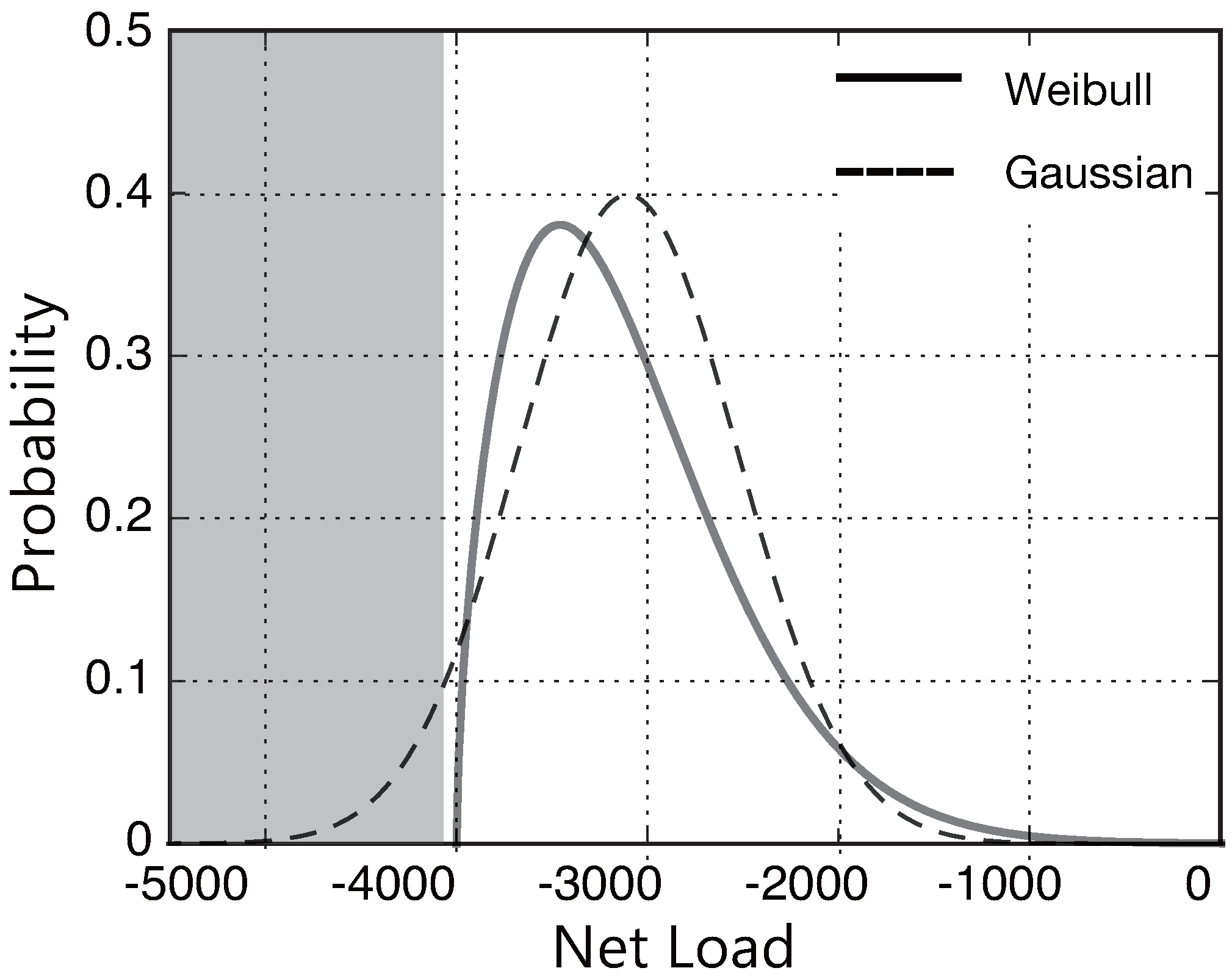
A few years ago, many researches approximated residential energy demand and residential renewable energy production using a Gaussian distribution [5]. However, as Munkhammar et al. [21] suggests, residential electricity consumption effectively follows the Weibull distribution. It is ofen the case that underestimate or overestimate of the risk occurs, if we incorrectly approximate the skewed real data using a Gaussian distribution. Figure 1 compares Gaussian distribution and Weibull distribution which have same mean value and same standard deviation. Despite there are not a cause for concern to occur the gray area, we are required to purchase the electricity to avoid the risk in case we employ the Gaussian approximation. In the storage management problem, underestimation and overestimation of the risk correspond to the over-discharging and over-charging risks, respectively. They would result in additional costs such as purchases at balancing market, opportunity loss, battery degradation and so on.

Figure 1. Gaussian and Weibull distributions with equal mean values and standard deviations.

Figure 1. Gaussian and Weibull distributions with equal mean values and standard deviations.

We employ the CVaR measure for the storage management problem to deal with non-normal predictive models on energy demand and productions. Our model is based on direct specification of θ for calculating CVaR ${\mathrm{E}}_X\left[X\right|X>\theta ]$ unlike in past researches [9,13] which employ the empirical percentage parameter α for CVaR such as 95%. Moreover, based on a CVaR measure, we can systematically design cost functions including the previous cost function Equation (7) [14].

2.2. Storage Management Problem

Let $l_h$ be a random variable of the net load per hour from time h. Let $s_h\in \mathcal{S}\subset \mathbb{R}$ be a variable of the state of charge (SOC) at time h. $\mathcal{S}$ is a closed set that $\mathcal{S}=[0,{\mathrm{S}}_{\max }]$ where ${\mathrm{S}}_{\max }$ is the battery capacity. Let $a_h\in \mathcal{A}\subset \mathbb{R}$ be a forward contract of the power purchase from time h to $h+1$ at the day-ahead market. $\mathcal{A}$ is a closed set that $\mathcal{A}=[0,{\mathrm{A}}_{\max }]$ where ${\mathrm{A}}_{\max }$ is the upper limit of the power purchase per unit of time. Let $p_h$ be a constant value of power price from time h to $h+1$ at the day-ahead market. Contract $a_h$ at the day-ahead market requires us to pay:

$$\begin{array}{c}\hfill C_{0,h}=p_h{a}_h\end{array}$$

(9)

To define the transition probability $\mathrm{Pr}\left(s_{h+1}\right|s_h,a_h)$, we define the event set under which over discharging occurs:

$$\begin{array}{c}\hfill {\mathbf{L}}_1=\left\{L\right|s_h+a_h+L\le 0,L\in \mathbb{R}\}\end{array}$$

(10)

We also define the event set under which over charging occurs:

$$\begin{array}{c}\hfill {\mathbf{L}}_2=\left\{L\right|{\mathrm{S}}_{\max }\le s_h+a_h+L,L\in \mathbb{R}\}\end{array}$$

(11)

The sets ${\mathbf{L}}_1$ and ${\mathbf{L}}_2$ are determined under a given value of $a_h$ and $s_h$.

We define transition probability toward $s_{h+1}=0$ as:

$$\begin{array}{c}\hfill \mathrm{Pr}(s_{h+1}=0|s_h,a_h,l_{h-1})={\int }_{{\mathbf{L}}_1}dL\mathrm{Pr}(l_h=L|l_{h-1})\end{array}$$

(12)

We also define transition probability toward $s_{h+1}={\mathrm{S}}_{\max }$ as:

$$\begin{array}{c}\hfill \mathrm{Pr}(s_{h+1}={\mathrm{S}}_{\max }|s_h,a_h,l_{h-1})={\int }_{{\mathbf{L}}_2}dL\mathrm{Pr}(l_h=L|l_{h-1})\end{array}$$

(13)

If $0<z_{h+1}=s_h+a_h+L<{\mathrm{S}}_{\max }$ is met, transition probability toward $s_{h+1}=z_{h+1}$ is defined as:

$$\begin{array}{c}\hfill \mathrm{Pr}(s_{h+1}=z_{h+1}|s_h,a_h,l_{h-1})=\mathrm{Pr}(l_h=L|l_{h-1})\end{array}$$

(14)

By marginalization, we get:

$$\begin{array}{c}\hfill \begin{array}{cc}& \mathrm{Pr}\left(s_{h+1}\right|s_h,a_h)=\int d{l}_0\dots d{l}_{h-1}\mathrm{Pr}\left(s_{h+1}\right|s_h,a_h,l_{h-1})\prod _{i=1}^{h-1}\mathrm{Pr}\left(l_i\right|l_{i-1})\hfill \end{array}\end{array}$$

(15)

We are exposed to the over discharging risk and the over charging risk in conjunction with contract $a_h$. We employ CVaR measure to evaluate these risk from time h to $h+1$. In other words, we employ the conditional expectation as we showed in Equations (1)–(3). Over discharging risk is calculated as:

$$\begin{array}{c}\hfill \begin{array}{cc}\hfill C_1(s_h,a_h,l_{h-1})=& -p_h\frac{{\int }_{{\mathbf{L}}_1}dL(s_h+a_h+L)\mathrm{Pr}(l_h=L|l_{h-1})}{{\int }_{{\mathbf{L}}_1}dL\mathrm{Pr}(l_h=L|l_{h-1})}\hfill \end{array}\end{array}$$

(16)

The over charging risk is similarly calculated as:

$$\begin{array}{c}\hfill \begin{array}{cc}\hfill C_2(s_h,a_h,l_{h-1})=& p_h\frac{{\int }_{{\mathbf{L}}_2}dL(s_h+a_h+L)\mathrm{Pr}(l_h=L|l_{h-1})}{{\int }_{{\mathbf{L}}_2}dL\mathrm{Pr}(l_h=L|l_{h-1})}\hfill \end{array}\end{array}$$

(17)

By marginalization, we get:

$$\begin{array}{c}\hfill \begin{array}{cc}\hfill C_k(s_h,a_h)=& \int d{l}_0\dots d{l}_{h-1}{C}_k(s_h,a_h,l_{h-1})\prod _{i=1}^{h-1}\mathrm{Pr}\left(l_i\right|l_{i-1})\hfill \end{array}\end{array}$$

(18)

where $k=1,2$.

Finally, we define the state value function $V^{\pi }\left(s_h\right)$ for a time horizon H. π is a deterministic policy set $\pi =\{{\pi }_h,{\pi }_{h+1},\dots ,{\pi }_{h+H}\}$ where ${\pi }_h:\mathcal{S}\to \mathcal{A}$. With the weight coefficients $w_1,w_2\in \mathbb{R}$, we define a loss function $L^{\pi }(s_h,a_h)$ as:

$$\begin{array}{c}\hfill \left\{\begin{array}{cc}{L}^{\pi }\left(s_h\right)=p_h{a}_h+w_1{C}_1(s_h,a_h)+w_2{C}_2(s_h,a_h)\hfill & \\ a_h={\pi }_h\left(s_h\right)\hfill \end{array}\right.\end{array}$$

(19)

Then, the state value function becomes:

$$\begin{array}{cc}\hfill V^{\pi }\left(s_h\right)& =L^{\pi }\left(s_h\right)+{\mathbb{E}}_{s_{h+1},\dots ,s_{h+H}}\left[\sum _{t=h+1}^{h+H}{L}^{\pi }\left(s_t\right)\right]\hfill \\ & =L^{\pi }\left(s_h\right)+{\int }_{\mathcal{S}}d{s}_{h+1}\mathrm{Pr}\left(s_{h+1}\right|s_h,a_h)V^{\pi }\left(s_{h+1}\right)\hfill \end{array}$$

(20)

The storage management problem is the minimization of the state value function $V^{\pi }\left(s_h\right)$ described in Equation (20). The optimal power contracts at the each SOC are obtained by minimizing Equation (20):

$$\begin{array}{c}\hfill {\pi }_h^{*}\left(s_h\right)\in \underset{a_h}{arg\; min}{V}^{\pi }\left(s_h\right)\end{array}$$

(21)

2.3. Discretized Storage Management Problem

In this study, the payments from two different predictive models are compared: one is a normal distribution and the other is a normalized frequency distribution. As the simple case, we employ the predictive models which have independence between adjacent net loads, such as $l_h$ and $l_{h+1}$. In what follows, we discretize the state space and action space of previous optimization problem.

2.3.1. State and Action Spaces

We described time of day using $\mathcal{H}=\{0,1,\dots ,\mathrm{H}\}$. Battery capacity is divided into $\mathrm{N}\in \mathbb{N}$ level. The battery level is represented by the elements of $\mathcal{S}=\{0,\Delta ,\dots ,\mathrm{N}\Delta \}$ with $\Delta ={\mathrm{S}}_{\max }/\mathrm{N}$ Wh. We define $s_h\in \mathcal{S}$ as a random variable corresponding to the remaining battery level at time h. We also discretize the admissible action space about the power purchases using set $\mathcal{A}=\{0,\Delta ,\dots ,\mathrm{A}\Delta \}$, where $\mathrm{A}\in \mathbb{N}$. Here, $\mathrm{A}\Delta$ is the upper limit of the power purchase per unit of time. Furthermore, we define $a_h\in \mathcal{A}$ be the amount of power purchase at time h.

2.3.2. Transition Probability

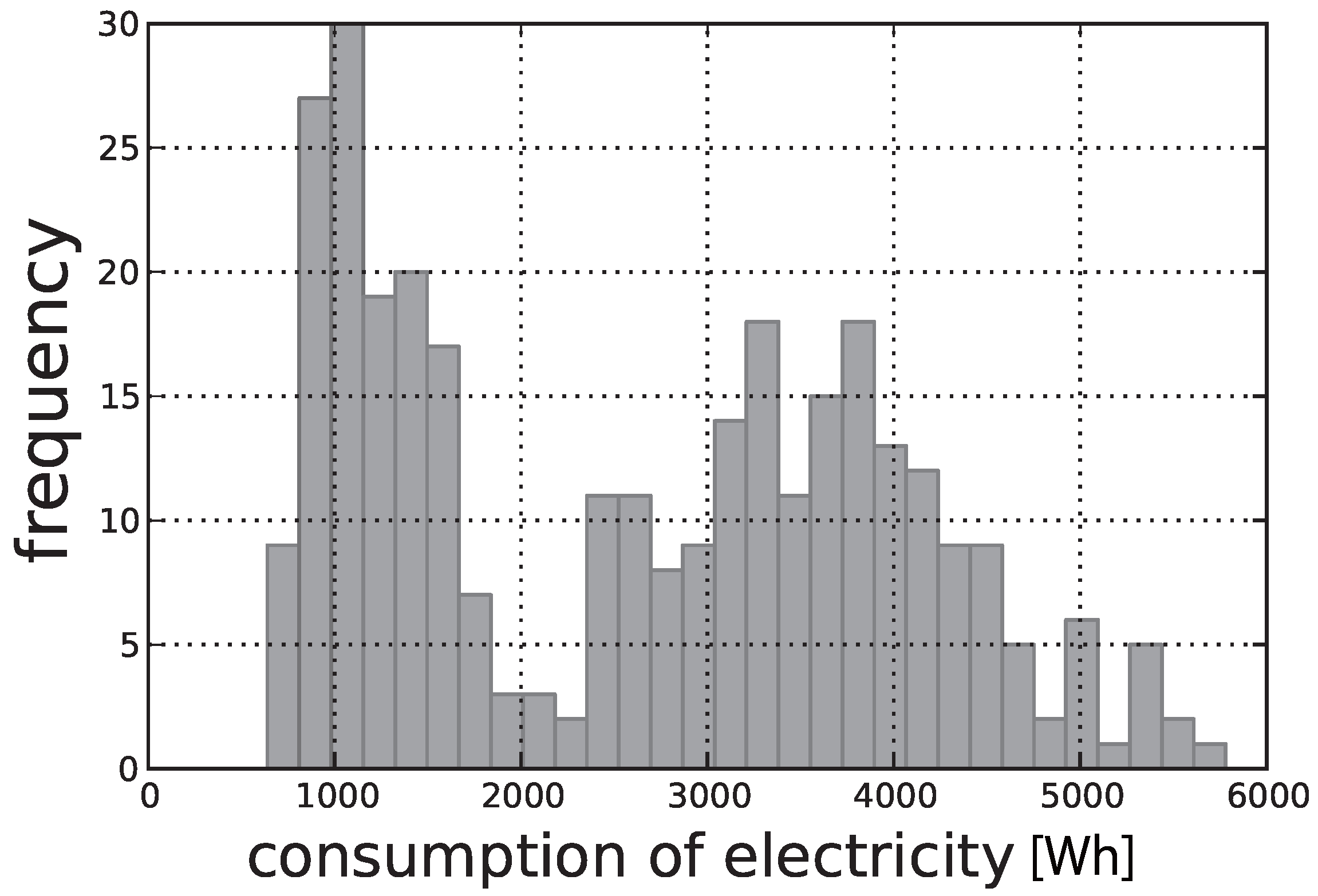
Given time $h\in \mathcal{H}$, the net load during time slot $[h,h+1)$ is defined by discrete random variable $l_h$. The probability measure of net load $l_h$ is modeled from the past d-days in time slot $[h,h+1)$ (e.g., Figure 2). The class interval of the distribution $\mathrm{Pr}\left(l_h\right)$ is adjusted to Δ.

Transition probability is calculated as follows:

$$\begin{array}{c}\hfill \mathrm{Pr}(s_{h+1}=0|s_h,a_h)=\sum _{L\in {\mathbf{L}}_1}\mathrm{Pr}(l_h=L)\end{array}$$

(22)

where ${\mathbf{L}}_1=\left\{k\right|0\ge k+s_h+a_h\},$ and:

$$\begin{array}{c}\hfill \mathrm{Pr}(s_{h+1}={\mathrm{S}}_{\max }|s_h,a_h)=\sum _{L\in {\mathbf{L}}_2}\mathrm{Pr}(l_h=L)\end{array}$$

(23)

where ${\mathbf{L}}_2=\left\{k\right|{\mathrm{S}}_{\max }\le k+s_h+a_h\}:$

$$\begin{array}{c}\hfill \mathrm{Pr}(s_{h+1}=s_h+a_h+L|s_h,a_h)=\mathrm{Pr}(l_h=L)\end{array}$$

(24)

otherwise.

Figure 2. Histogram of the energy consumption from 7:30 a.m. to 8:00 a.m. for a representative household.

Figure 2. Histogram of the energy consumption from 7:30 a.m. to 8:00 a.m. for a representative household.

2.3.3. Loss Function and Bellman Equation

We let $p_h$ (yen/Wh) represent the power price during $[h,h+1),h\in \mathcal{H}$. We define the loss function $l(s_h,a_h)$ as:

$$\begin{array}{cc}\hfill l(s_h,a_h)=p_h{a}_h& -p_h{w}_1\frac{{\sum }_{L\in {\mathbf{L}}_1}(s_h+a_h+L)\mathrm{Pr}(l_h=L)}{{\sum }_{L\in {\mathbf{L}}_1}\mathrm{Pr}(l_h=L)}\hfill \\ & +p_h{w}_2\frac{{\sum }_{L\in {\mathbf{L}}_2}(s_h+a_h+L)\mathrm{Pr}(l_h=L)}{{\sum }_{L\in {\mathbf{L}}_2}\mathrm{Pr}(l_h=L)}\hfill \end{array}$$

(25)

Here, $w_1$,$w_2\in \mathbb{R}$ are the weight coefficients for the constraint regulation cost. Using these weight coefficients, we can represent the cost as:

• the incurred maintenance cost due to the deteriorating effect of battery overcharge and over-discharge or
• the incurred recourse cost due to the additional requirement of an intraday trading payment from the previous day’s trading payment.

The purpose of this MDP is to develop a power purchase program that minimizes the daily electric bill. The optimal state value function, $V^{*}\left(s_h\right)$, is determined by solving the following Bellman equation:

$$\begin{array}{c}\hfill V^{*}\left(s_h\right)=\underset{a_h}{min}\left\{Q(s_h,a_h)\right\}\end{array}$$

(26)

in which $Q(s_h,a_h)$ is defined as:

$$\begin{array}{c}\hfill Q(s_h,a_h)=l(s_h,a_h)+\sum _{s_{h+1}\in \mathcal{S}}\mathrm{Pr}\left(s_{h+1}\right|s_h,a_h)V^{*}\left(s_{h+1}\right)\end{array}$$

(27)

The optimal amount of power purchase at the state $s_h$ can be derived:

$$\begin{array}{c}\hfill {\pi }^{*}\left(s_h\right)=min\left\{\underset{a_h}{arg\; min}\left\{Q(s_h,a_h)\right\}\right\}\end{array}$$

(28)

Solution Equation (28) enable us to minimize the electricity bill payment.

3. Numerical Experiments

We compare the annual electricity bill payments result from daily storage operation based on two predictive probability distributions: the frequency distribution and the Gaussian distribution.

At first, we explain about data. Next, we show that the data is not normally distributed. At last, we present results of annual electricity bill payments.

3.1. Data

In this study, we use the Japanese residential time course dates for photovoltaic generation and electricity consumption, which were monitored from October 2010 to September 2011, for 35 households in Shiga, Japan [22]. The households were sampled every 30 min.

3.2. Normality Tests and Results

As mentioned in Section 2.3, we modeled the predictive distribution for the net load as an independent and identically distributed (IID) process. In other words, the predictive distribution are determined for each hour independently. For the numerical experiments, we prepared 24 histograms or 24 gaussian distributions as a daily predictive distribution from past 30 days data. A total of 24 (h) × 320 (days) = 7680 distributions were prepared for each household.

We tested the normality of the 7680 histograms using the Shapiro-Wilk test. This test checks the null hypothesis that samples are generated from normal distribution. We set significance level $\alpha =$ 0.05. The test is applicable to approximately 30 sample sizes [23].

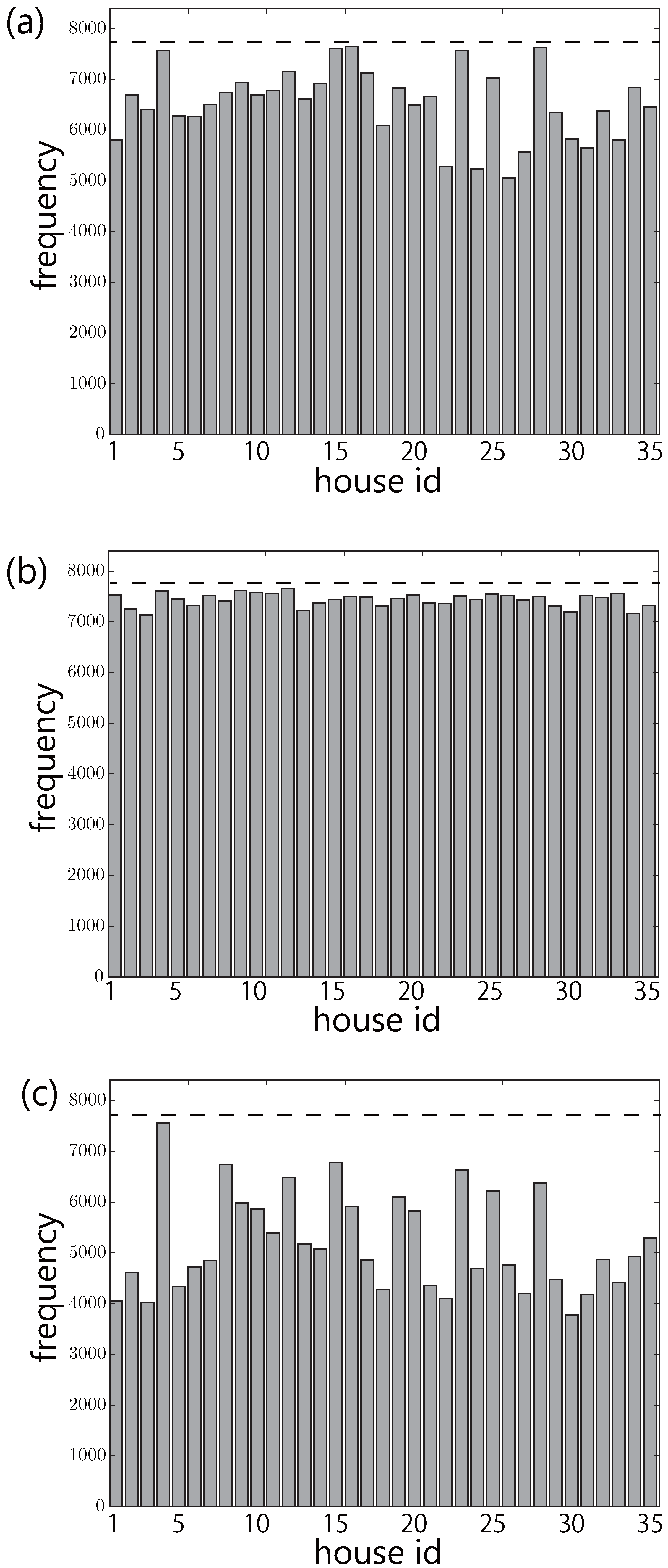
Figure 3a,c shows the results of the Shapiro-Wilk normality test. We applied this test not only for net load but also for electricity consumption and PV generation. Figure 3a is the result about electricity consumption. Y-axis shows the number of null hypothesis rejection and X-axis shows the household number. An average of 6528 histograms are rejected. Figure 3b is about PV power generation. An average of 7437 histograms are rejected. Figure 3c is about net load. An average of 5196 histograms are rejected. The binomial two-sided test with significance level $\alpha =$ 0.05 confirmed that all these results are significant.

In summary, we can say that the 30-day histogram of net load is not normal.

Figure 3. The results of normality test for (a) electricity consumption; (b) photovoltaics (PV) generation; and (c) net load. Y-axis shows the number of non-normal histograms. Dotted lines show the total number of histograms that were tested.

Figure 3. The results of normality test for (a) electricity consumption; (b) photovoltaics (PV) generation; and (c) net load. Y-axis shows the number of non-normal histograms. Dotted lines show the total number of histograms that were tested.

3.3. Conditions

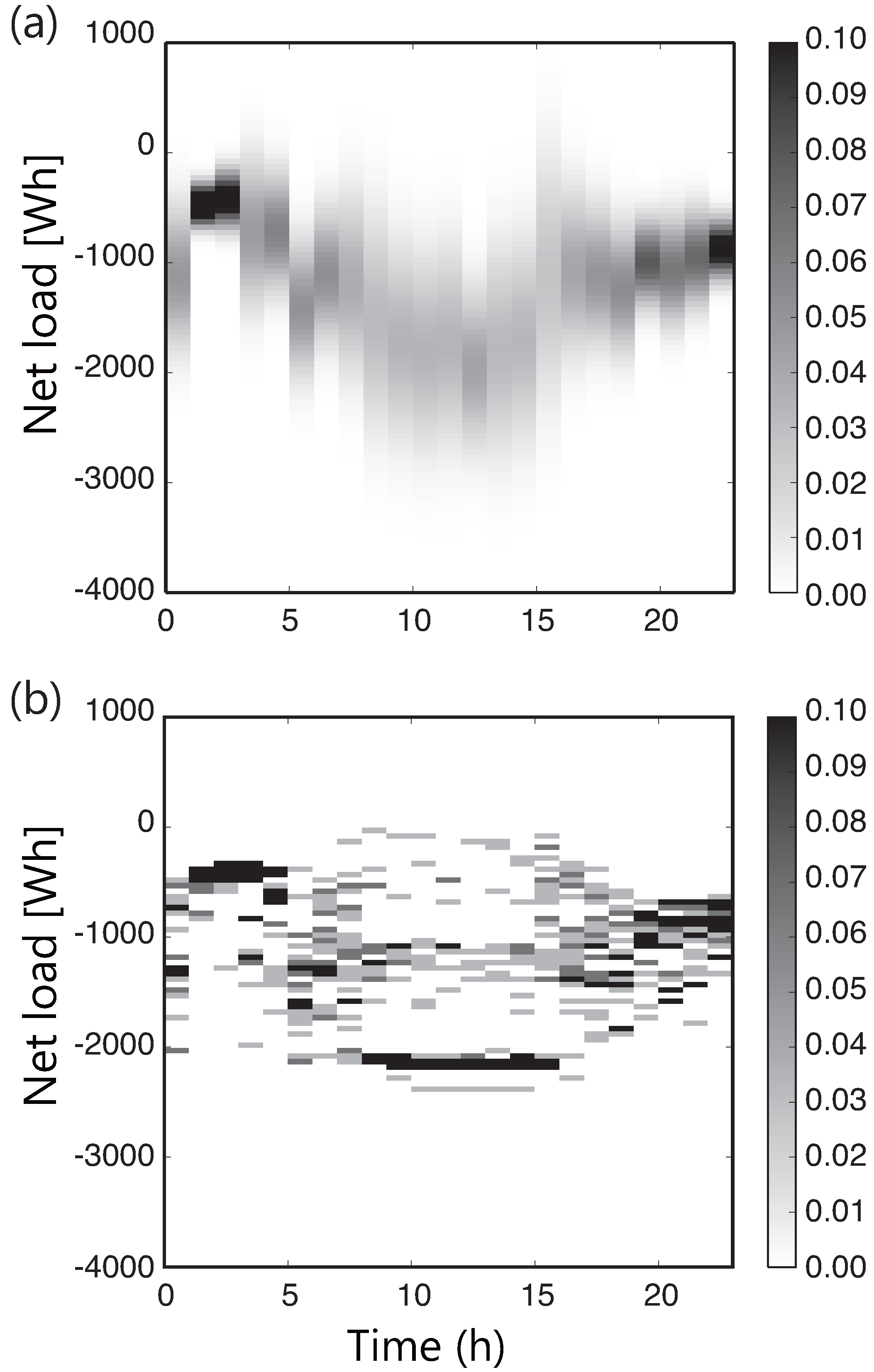
The predictive probability distribution of net loads was calculated from the most recent 30 days for each house and for each day. As we have discussed, one of the predictive distributions employed here is the normalized frequency distribution. As a control group for this predictive distribution, we prepared the normal distributions with mean and variance calculated from the most recent 30 days (Figure 4a). Corresponding normalized frequency distribution is illustrated in Figure 4b.

Figure 4. Prediction probability distributions of the efficient load over time using the normal distribution.

Figure 4. Prediction probability distributions of the efficient load over time using the normal distribution.

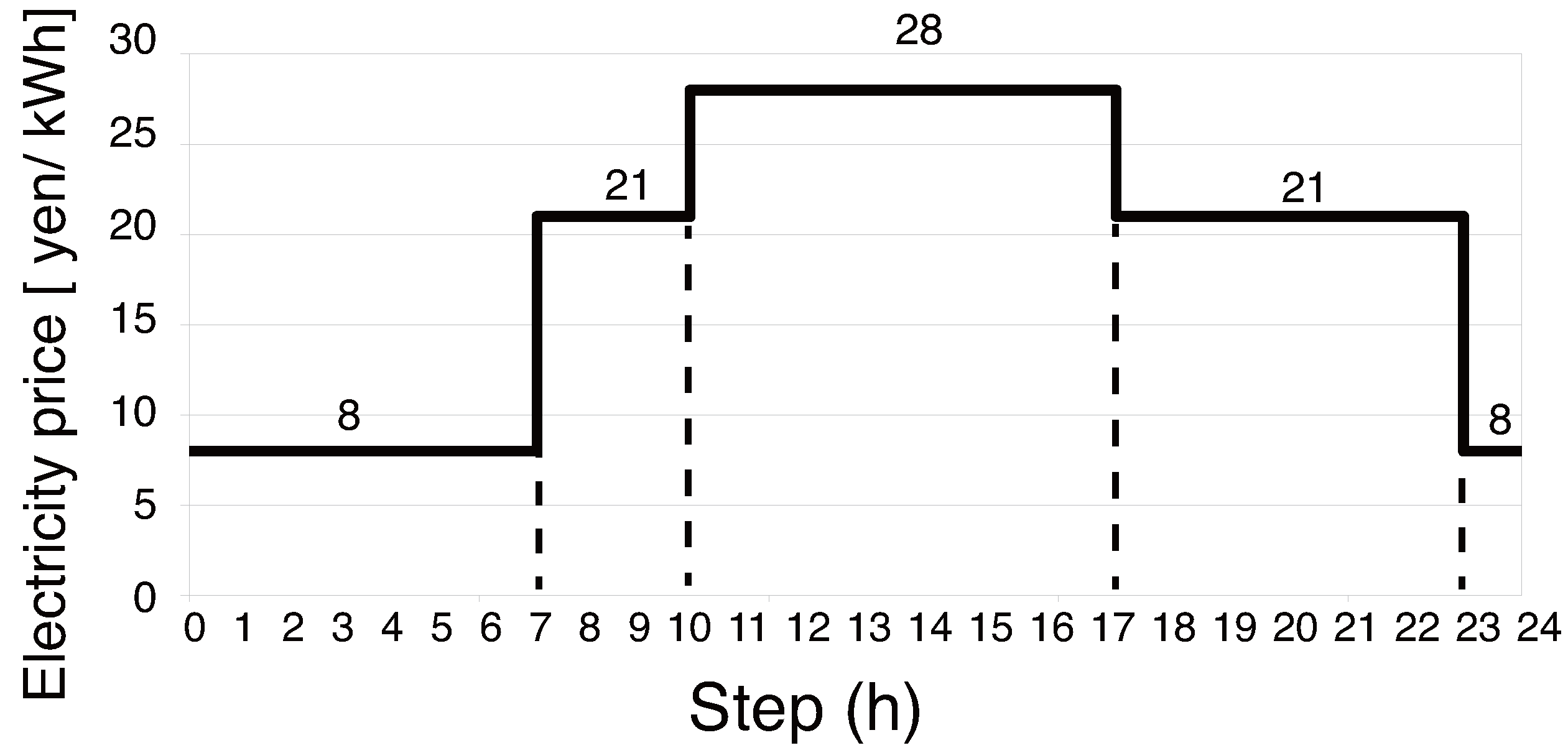
We set a power prices based on the time-of-use plan provided by Kansai Electric Power Co., Inc., Japan (Figure 5).

To consider the storage capacity, we prepared the following six cases: ${\mathrm{S}}_{\max }\in \{$2000, 4000, 6000, 8000, 10,000, 15,000} Wh. For each case, we fix $\Delta =10$ Wh. The predictive probability distribution for the first day is determined using the data between 1 and 31 October.

Figure 5. Price of electricity provided by power plant.

Figure 5. Price of electricity provided by power plant.

Furthermore, we consider the following two parameter cases: $(w_1,w_2)=(1.0,0.0)$ and $(w_1,w_2)=(10.0,0.0)$. These parameters adjust the constraint regulation cost. The first setting corresponds to the case in which additional cost is not required. Electricity is available at the same cost if over-discharging occurs. The second setting corresponds to the case in which additional cost is required if over-discharging occurs. In these computational example, we ignored the over-charging cost: $w_2=0$.

The annual electricity bill payments are calculated for 35 households.

3.4. Algorithms

We apply a backward induction method (Algorithm 1) to solve the MDP defined in Section 2.3.

In Algorithm 1, lines 1 through 3 initialize the state value function. Subsequently, lines 4–8 update the state value for each state, and line 9 determines the optimal amount of power purchase.

Algorithm 1 Backward induction

1: for $h=0$ to H do 2:   for $s_h\in \mathcal{S}$ do 3:       V($s_h$)=0 4:   end for 5: end for 6: for $h=$H$-1$ to 0 do 7:   for $s_h\in \mathcal{S}$ do 8:       $V^{*}\left(s_h\right)={min}_{a_h}\left\{Q(s_h,a_h)\right\}$ 9:       ${\pi }^{*}\left(s_h\right)=min\left\{{arg\; min}_{a_h}\left\{Q(s_h,a_h)\right\}\right\}$ 10:   end for 11: end for

Proposed problem is solved by the model-predictive manner. We are required to alternate updating predictive models and solving the planning problem. Predictive distribution of the net load must be updated using the previous d-days at the end of each day. Then we determine the optimal power purchase actions of the next day.

The realized net load and the charge state on the day are not discretized. Therefore, we employ the projection on the discretized state space ${\tilde{s}}_h^{*}={arg\; min}_{s_h\in {\mathcal{S}}_h}|s_h-{\tilde{s}}_h|$ where ${\tilde{s}}_h$ represents the realized SOC. Then power purchase corresponds to ${\tilde{s}}_h$ is determined based on prior planning. If realized net load causes over-discharge or over-charge, a charge control is employed to maintain $0\le {\tilde{s}}_h\le {\mathit{S}}_{\max }$.

4. Results

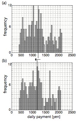
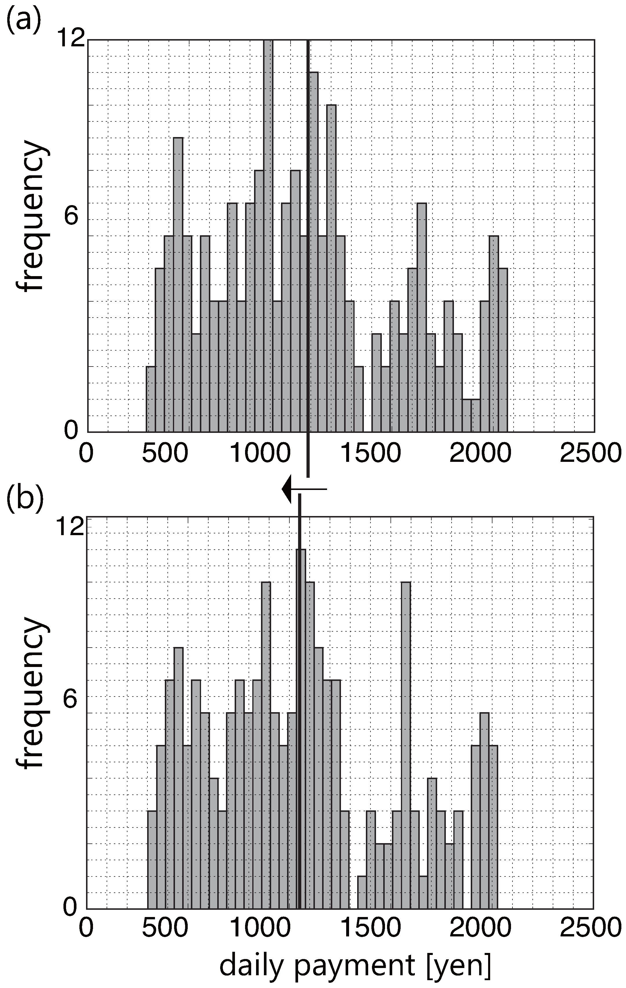
Figure 6 provides an example of the results. This figure shows the annual histogram of the daily payments calculated for a single house with ${\mathit{S}}_{\max }=6000$ Wh and $w_1=1.0$. Histogram (a) is calculated using the Gaussian predictive distributions. Histogram (b) is calculated using the normalized frequency distributions. As shown in the histograms, the mean value of the daily payments is improved by controlling the risk from non-normality.

Figure 6. The household’s daily payments for one year calculated using (a) the gaussian predictive distributions and (b) the normalized frequency distributions. Bold vertical line shows the mean value of each histogram.

Figure 6. The household’s daily payments for one year calculated using (a) the gaussian predictive distributions and (b) the normalized frequency distributions. Bold vertical line shows the mean value of each histogram.

To test the statistically significant improvement in the average of payment histograms, we checked the normality of each histograms. We apply the Shapiro-Wilk test to every payment histograms. The null hypothesis is that the distribution is normal. Table 1 shows the number of households in which the null hypothesis was rejected.

Table 1. Fraction of the 35 households in which the null hypothesis was rejected.

Storage	Weight = 1.0		Weight = 10.0
	Gauss	Nonparametric	Gauss	Nonparametric
2000 Wh	23/35	23/35	32/35	33/35
4000 Wh	21/35	20/35	31/35	34/35
6000 Wh	21/35	23/35	33/35	32/35
8000 Wh	19/35	19/35	31/35	32/35
10,000 Wh	19/35	19/35	33/35	31/35
15,000 Wh	19/35	19/35	30/35	30/35

Table 1. Fraction of the 35 households in which the null hypothesis was rejected.

Storage	Weight = 1.0		Weight = 10.0
	Gauss	Nonparametric	Gauss	Nonparametric
2000 Wh	23/35	23/35	32/35	33/35
4000 Wh	21/35	20/35	31/35	34/35
6000 Wh	21/35	23/35	33/35	32/35
8000 Wh	19/35	19/35	31/35	32/35
10,000 Wh	19/35	19/35	33/35	31/35
15,000 Wh	19/35	19/35	30/35	30/35

For instance, if we operate the storage management using Gaussian predictive distribution with 2000 Wh storage capacitor under risk weight $w_1=1.0$, the annual payment histogram of 23 households out of 35 households are non-normal. In summary, only about 30% of the data were normal (Table 1).

We applied a nonparametric test, called the one-sided Wilcoxon signed-rank test, to test the statistically significant improvement in the payment histograms. Null hypothesis is that there is no difference between the medians of the given two distributions. Alternative hypothesis is that the median of the normalized frequency distribution is less than that of the normal distribution. We set the level of significance to $\alpha =$ 0.05.

Table 2 shows the results of the one-sided Wilcoxon signed-rank test. First row shows the calculation conditions about storage capacitor. Second row shows the number of households that improved the payments by using the frequency distribution. Third row shows the cost-saving improvement rate which is calculated from the median values. For instance, if we operate the storage management using the frequency distribution with 15,000 Wh storage capacitor under risk weight $w_1=$ 1.0, we can save the annual payment in 34 households out of 35 households with average 0.98 times. We added asterisk in the second row when the number of improved households were statistically significant. The two-sided binomial test was used to check this significance. When storage capacitor is greater than or equal to 6000 Wh, statistically-significant superiority of considering non-normality appears. As can be observed in the third row, the effectiveness of the frequency distribution increases with an increase in the storage amount. The rate of improvement was from 1% to 10%.

Table 2. Comparison of annual payments.

Storage	Weight = 1.0		Weight = 10.0
	Number of improved houses	Performance (35-house average)	Number of improved houses	Performance (35-house average)
2000 Wh	21/35	1.00	23/35 *	1.04
4000 Wh	19/35	1.01	19/35	1.07
6000 Wh	24/35 *	0.99	21/35	1.03
8000 Wh	30/35 *	0.98	23/35 *	0.97
10,000 Wh	33/35 *	0.98	27/35 *	0.93
15,000 Wh	34/35 *	0.98	29/35 *	0.90

“*” means there were a significant number of improved houses with significance level $\alpha =$ 0.05.

Table 2. Comparison of annual payments.

Storage	Weight = 1.0		Weight = 10.0
	Number of improved houses	Performance (35-house average)	Number of improved houses	Performance (35-house average)
2000 Wh	21/35	1.00	23/35 *	1.04
4000 Wh	19/35	1.01	19/35	1.07
6000 Wh	24/35 *	0.99	21/35	1.03
8000 Wh	30/35 *	0.98	23/35 *	0.97
10,000 Wh	33/35 *	0.98	27/35 *	0.93
15,000 Wh	34/35 *	0.98	29/35 *	0.90

“*” means there were a significant number of improved houses with significance level $\alpha =$ 0.05.

5. Conclusions

In this paper, we formulated the economically optimal storage control problem using Markov decision process (MDP) and the CVaR measure to deal with the non-normality of predictive distribution about the household’s net load. Non-normality of the net load has the possibility to cause the battery overcharge risk and over-discharge risk in a characteristic fashion. CVaR measure was employed to treat with these risks.

We checked the superiority of the proposed MDP to deal with non-normality of transition probability distribution. We compared the economic saving performances between two MDPs: one is the MDP with a Gaussian predictive distribution and the other is the MDP with a normalized frequency distribution. Our calculations indicate the annual savings among the households increase up to 10% when we employ the proposed MDP using the normalized frequency distribution rather than the normal distribution. Although we observed few case that MDP using the normalized frequency worsen the annual saving, there are at least two things to note here. One is about the predictive distribution: we have enough options other than normalized frequency distribution. The normalized frequency distribution was employed just as an example to show the capability of proposed MDP to deal with non-normality in this paper. It would be fruitful to explore the other predictive distributions effective for the annual savings of payments. The other is about a chance to choice the appropriate predictive model. If residents simulate their annual payments using the previous year data, it is easy to choose the appropriate predictive distributions, the storage capacitor and so on, for the following year.

At the end of this paper, we pick up an issue in the future. The considered market in the proposed MDP was the one where we can purchase the electricity at any given time with deterministic price. The proposed MDP is inapplicable to the market where the electricity is provided with the stochastic price such as the balancing market. A number of research dealing with this stochasticity are already existing. Introducing the stochasticity of the power price into the loss function and policy would be required in the future.