Article

Integrating Auto-Associative Neural Networks with Hotelling T2 Control Charts for Wind Turbine Fault Detection

Department of Industrial Engineering and Management, National Chin-Yi University of Technology, Taichung City 41170, Taiwan
*
Author to whom correspondence should be addressed.
Energies 2015, 8(10), 12100-12115; https://doi.org/10.3390/en81012100
Submission received: 6 September 2015 / Revised: 9 October 2015 / Accepted: 19 October 2015 / Published: 23 October 2015
(This article belongs to the Special Issue Wind Turbine 2015)

Abstract

:
This paper presents a novel methodology to detect a set of more suitable attributes that may potentially contribute to emerging faults of a wind turbine. The set of attributes were selected from one-year historical data for analysis. The methodology uses the k-means clustering method to process outlier data and verifies the clustering results by comparing quartiles of boxplots, and applies the auto-associative neural networks to implement the residual approach that transforms the data to be approximately normally distributed. Hotelling T2 multivariate quality control charts are constructed for monitoring the turbine’s performance and relative contribution of each attribute is calculated for the data points out of upper limits to determine the set of potential attributes. A case using the historical data and the alarm log is given and illustrates that our methodology has the advantage of detecting a set of susceptible attributes at the same time compared with only one independent attribute is monitored.

1. Introduction

Wind energy has become one of major sources of renewable energy because of growing environmental concerns. A wind turbine extracts energy from the wind and the amount of energy extracted depends largely on the wind speed. The power generated by a turbine at various wind speeds is described by a power curve that resembles a sigmoid function. Due to the stochastic nature of wind, main components of wind turbines like blades and generators are susceptible to various types of faults. The frequency and severity of the faults affect operations and maintenance costs, and unscheduled shutdowns are costly. Condition and performance monitoring methodologies have been developed to detect early faults and reduce unscheduled shutdowns; reviews of the proposed methodologies and future research trends are provided [1,2,3].
Condition and performance monitoring based on data mining and statistical methods are developed in several studies [2]. More recently, a multivariate outlier detection approach and the use of Hotelling T2 control charts to monitor the performance of wind turbines was proposed [4]. Integrating the residual approach [5] for monitoring the power curves with auto-associative neural networks (AANN) to detect the attribute contributing to faults was proposed [6]. Motivated by [4,6], this paper proposes a three-phase methodology to detect a set of potential attributes contributing to emerging faults. The first phase processes outliers by using the k-means clustering method, and justifies the results by comparing both the first and the third quartiles of boxplots before the clustering to those after the clustering. The second phase applies the AANN to implement the residual approach that transforms the data to be approximately normally distributed. The third phase constructs the Hotelling T2 quality control charts using the data from the second phase and calculates relative contribution of each attribute for the data points out of upper limits. A case using the historical data collected from the supervisory control and data acquisition (SCADA) systems of a wind turbine is given to illustrate the methodology.
Using the residual approach for performance and condition monitoring of the wind farm and wind turbine are presented [6,7,8,9,10]. The AANN is implemented by training artificial neural networks (ANN) to perform the mapping by which each output target is approximated to each input attribute [11]. This one-to-one approximation makes the AANN a useful tool for measuring whether the output target has significantly deviated from the input attribute. Applications of AANNs to fault detection are presented by [12,13,14,15,16].
Our major contributions and comparisons with [4,6] are described as follows: first and foremost, to the best of our knowledge, the integration of the AANN and Hotelling T2 method has not been studied in the literature. Real contributions of the integration lie in the one-to-one mapping of the AANN to produce approximately normally distributed residuals that can be used to construct the Hotelling T2 control charts for monitoring multivariate simultaneously. Second, the proposed methodology in this paper differs from that presented in [4] in three aspects: (1) only bivariate data, which are kurtosis and skewness, were considered in [4]; (2) the data were normalized using the Box-Cox transformation in [4]; and (3) no significant pattern in the T2 statistic was observed in [4] and thus no subsequent discussions on how to identify the attributes contributing to data points out of limits. In addition, compared with [6], the proposed methodology improves in three aspects: (1) healthy data are obtained by using the k-means clustering method rather by selecting manually in [6]; (2) the multivariate Hotelling T2 statistic is computed instead of ranking mean square error (MSE) of the univariate to study only one attribute at a time in [6]; (3) when the faults occur are available from the control charts in this paper, while the power curve cannot provide such information in [6].
Because the Hotelling T2 control charts consider multivariate simultaneously, answering which of the attributes (or which subset of them) is contributing to an out-of-limit data point is not always easy [5]. A number of approaches proposed in the literature to diagnosis of an out-of-limit data point are discussed ([5], pp. 520–521). On the basis of these discussions, we choose to use the approach that decomposes the T2 statistic into components reflecting the contribution of each individual attribute [5]. The remainder of this paper is organized as follows: Section 2 describes the dataset, Section 3 introduces the proposed methodology, Section 4 presents and discusses the results, and Section 5 concludes the paper.

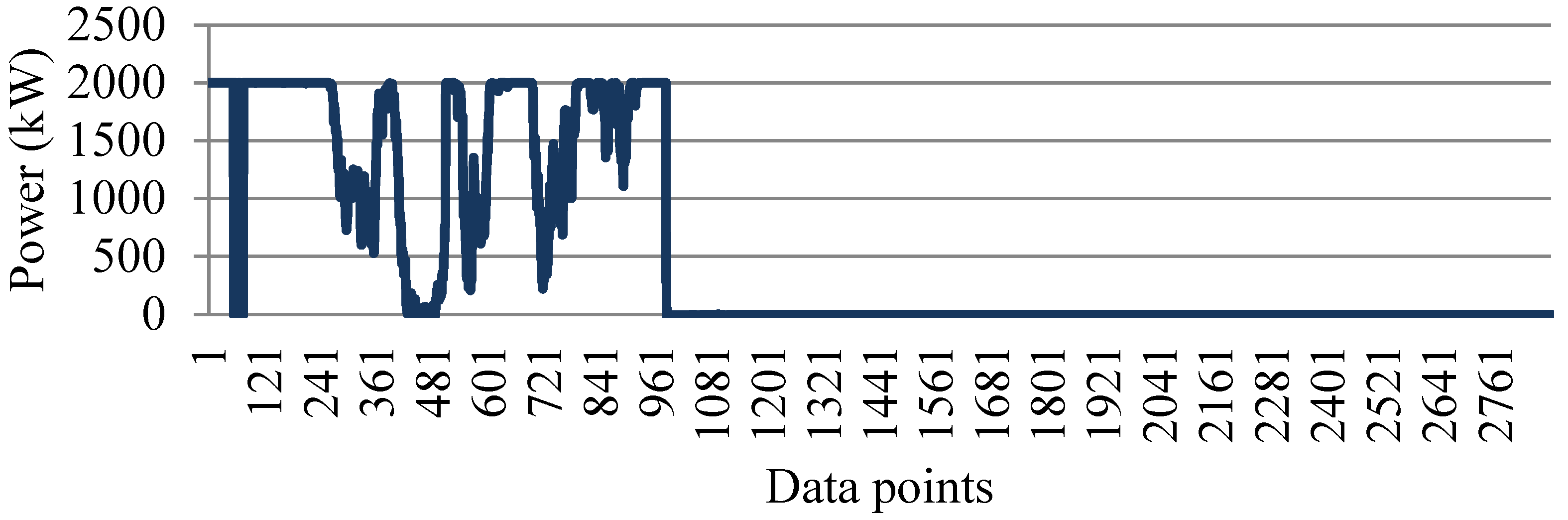
2. Dataset Description

The data used in this paper were collected from the SCADA systems of a 2.0 MW wind turbine located on the coast of central western Taiwan. An alarm log was also collected. The SCADA systems record more than 120 wind turbine attributes and the alarm log provides status and fault information. In this paper, we select a subset of attributes from [6] for analysis. The selection is determined mainly by preliminary studies on the alarm log, which reveals that the majority of the turbine faults are related to this subset. With such a subset of attributes, one may raise concern about the dataset used for the validation of the proposed methodology. Attribute extraction is a critical step in machine learning problems, whether classification or regression [17]. In general, important attributes can be selected initially with using domain knowledge and finally with data mining algorithms. Previous studies have applied data mining algorithms, such as ANN, support vector machines (SVM), and ensemble classifiers, to extract important information from the data [18]. However, past studies also used the methodology that selects only certain related attributes based on the literature and domain knowledge in wind energy [19,20]. In addition, standard technique used nowadays for fault diagnosis in wind turbines is to identify critical attributes by an expert and to develop a regression model to predict the failure [18]. Zaher et al. [20] mentioned that the methodology developed in their study can be applied by wind farm operators. The explanations above can justify our use of the dataset.
A set of example statistics from January 2009 is provided in Table 1 to illustrate the magnitudes of the attributes, where “Components or subsystems” refers to [21]. Examples of a partial alarm log are provided in Table 2. As certain faults are relatively rare, the imbalance level between the alarm logs and normal performance of the wind turbine state data not only makes early prediction of fault difficult but also is considered an open issue in machine learning and data mining applications. General techniques to balance the dataset include: (1) oversampling; (2) undersampling; (3) threshold moving; (4) ensemble techniques [22]. Techniques to balance the dataset are not implemented in this paper and the discussion of the final analysis will be given later.
The SCADA data in this paper were collected at 10-min intervals from 1 January 2009 to 31 December 2009, and the most recent data are not available for this study. For the turbine selected, the cut-in speed is 4 m/s, the rated speed is 16 m/s, and the cut-out speed is 25 m/s. The average wind speeds recorded by the turbine were 7.96 m/s.
Table 1. Attributes selected and their basic statistics for January 2009.
NumberComponents or SubsystemsName of AttributesUnitMinimumMaximumAverageStandard Deviation
1MeteorologyWind speedm/s0.326.512.195.97
2Rotor systemPitch angle°−2.389.569.6733.53
3GearboxGear bearing temperature°C158933.8919.04
4GearboxGear oil temperature°C177932.2515.43
5ConverterPower outputkW−21.52000.8328.81695.76
6GeneratorGenerator bearing temperature°C127828.8620.24
7GeneratorGenerator speedrpm01972427.86784.43
8Rotor systemRotor speedrpm016.33.436.54
Table 2. Sample of partial alarm log.
DescriptionDetectedLog Type
Pause pressed on keyboard21 January 2009, 02:56:29Alarm log
Start auto-outyawing23 February 2009, 05:02:32Alarm log
High wind speed: 25.1 m/s13 March 2009, 09:41:26Alarm log

3. Research Methodology

The research methodology is shown in Figure 1 and each phase is described in subsequent sections.
Figure 1. Research methodology.
Energies 08 12100 g001

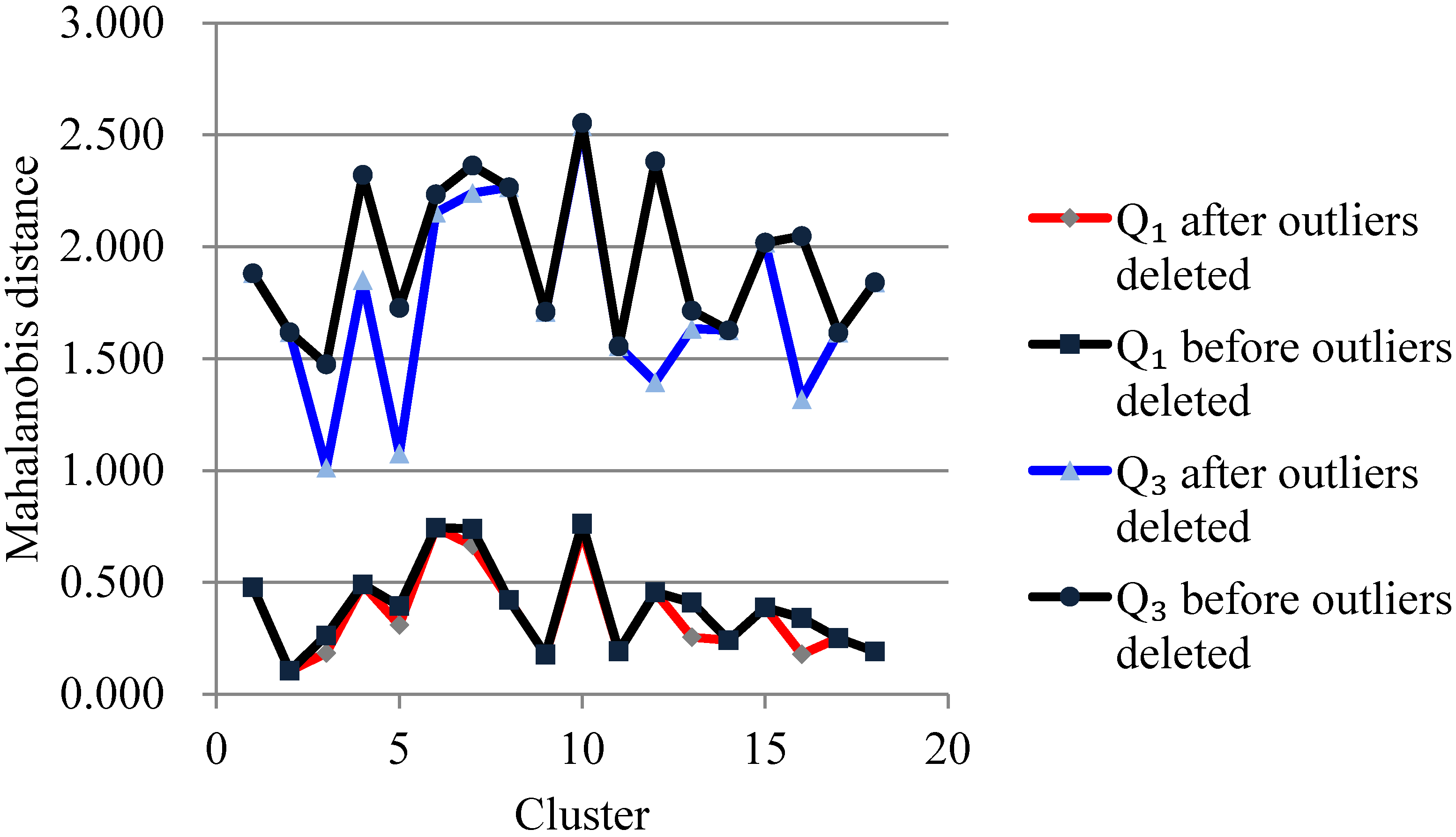
3.1. Processing Outliers

Outliers are largely due to stochastic nature of wind or sensor errors and affect the prediction accuracy of the model if they are not well processed. To delete outliers for constructing a normal behavior, a multivariate detection approach using Mahalanobis distance was proposed in [4]. Let Dij denote Mahalanobis distance between instances xi and xj, then Dij is calculated as the following:
D i j = ( x i x j ) T S 1 ( x i x j ) , i j
where S−1 is the inverse of covariance matrix. Simply calculating Mahalanobis distance can be misleading in the sense that data points close to cut-in wind speed, or/and near rated wind speed are considered as outliers but in fact they are not [4]. Therefore, data are grouped into smaller clusters to improve the detection of outliers. In this paper we follow the approach presented by [4] that applies the k-means clustering algorithm to group each attribute into smaller clusters, but we additionally use the first and the third quartiles of boxplots to verify whether the clustering results are improved after deleting outliers.

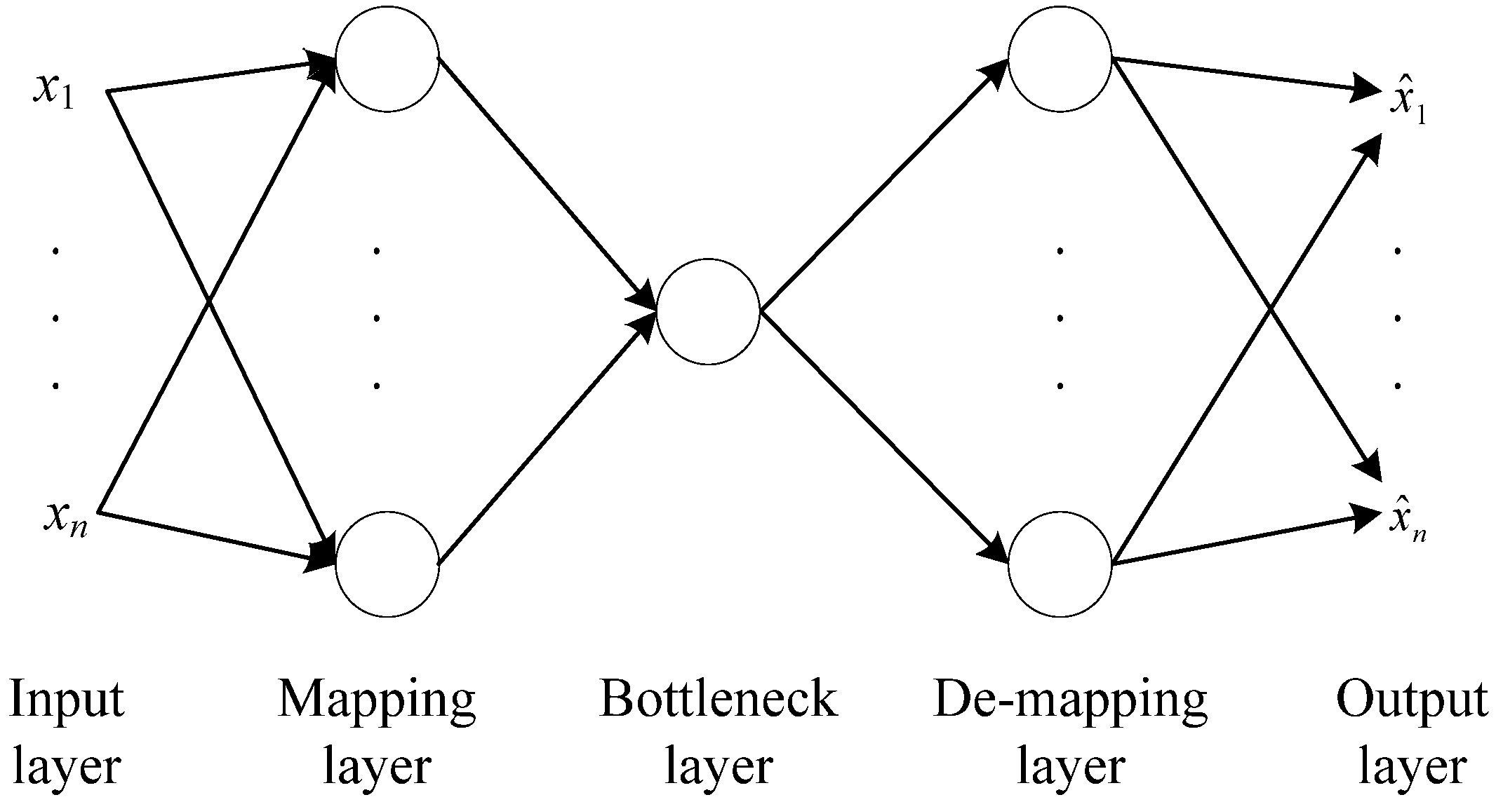
3.2. Auto-Associative Neural Networks (AANN) Model

A typical AANN model consists of five layers: an input layer, a mapping layer, a bottleneck layer, a de-mapping layer, and an output layer (Figure 2). In the context of the ANN model, the mapping layer, bottleneck layer, and de-mapping layer are classified as hidden layers. The AANN operates by training a feed-forward ANN to perform the mapping, where the input data are approximated at the output layer. If the number of nodes in the mapping and de-mapping layers are both k and the number of nodes in the bottleneck layer is p, the network is referred to as n-k-p-k-n, as shown in Figure 2, and we will use this representation below. The number of nodes in the mapping and de-mapping layers are equal and, in general, greater than the number of nodes in the input and output layers.
Figure 2. Structure of an auto-associative neural networks (AANN).
Energies 08 12100 g002
The bottleneck layer plays a central role in forcing the network to develop a reduced representation for the input data. The AANN uses a nonlinear function to map from the higher-dimension input space to the lower-dimension bottleneck space, followed by an inverse mapping from the bottleneck space back to the space represented by the output layer [11]. Due to the mapping from higher to lower-dimensions, the bottleneck layer contains fewer nodes than the input and output layers and extracts important attributes by eliminating redundant and insignificant data. After the network is trained to map the input data onto itself through the bottleneck layer, the network should be able to map new data that was unused for training. As long as the new data and the training data are from the same source, failure to map the new data suggests that the attributes may have changed and thus increases the magnitude of the residuals between the new data and the trained data.
The selection of the number of nodes in the bottleneck layer determines the order of reduction. To select the number of nodes in the bottleneck layer, the fraction of explained variance (FEV) was proposed in [23] as follows:
FEV = E [ x ^ ( t ) 2 ] E [ x ( t ) 2 ]
where x(t) is the input vector and x ^ ( t ) is the reduced vector.
The FEV indicator is analogous to the eigenvalues of the covariance matrix that explain the percentage captured by the principal component analysis. To attain a prescribed FEV, the number of nodes in the bottleneck layer is gradually increased during the training process until the prescribed FEV is achieved [23].
To measure the residuals between the input vector (x1, …, xn) and the output vector ( x ^ 1 , , x ^ n ), as shown in the example in Figure 2, we compute their MSE according to the following expression:
MSE = 1 n i = 1 n ( x i x ^ i ) 2
In general, there exists an inverse relationship between the MSE and the FEV, such that the larger FEV, the smaller MSE, and vice versa. The relationship simply describes that more nodes in the bottleneck layer correspond to a smaller error between (x1, …, xn) and ( x ^ 1 , , x ^ n ). In theory, if p equals to n, then the MSE is approximately zero and the FEV is approximately one.

3.3. Hotelling T2 Control Charts

Simultaneous monitoring more than one quality attribute in practice is common, which means that monitoring attributes independently could be misleading. In this paper, we consider multivariate process monitoring using the Hotelling’s control chart. For the subgroup size n = 1, the Hotelling T2 statistic is calculated as [5]:
T 2 = ( x x ¯ ) T S 1 ( x x ¯ )
where x is the observation vector, x ¯ is the sample mean vector, and S−1 is the inverse of covariance matrix.
The upper control limit (UCL) is calculated as the following [5]:
UCL = p ( m + 1 ) ( m 1 ) m 2 m p F α   ,   p   ,   m     p
where m is the number of samples, p is the number of attributes, and Fα, p, mp is obtained from F distribution.
To interpret out-of-control observations, one can decompose the T2 statistic into components that reflect the contribution of each independent attribute [5]. Let T2 be the value of the overall statistic, and T ( i ) 2 be the value of the statistic for all attributes excluding the i-th one. Then:
d i = T 2 T ( i ) 2
is the relative contribution of the i-th attribute to the overall statistic. When an out-of-control data point occurs, computing di and focusing on those relatively large attributes can be useful for the detection of anomaly.

4. Results and Discussion

This section discusses the results of processing outliers, training the AANN model, and constructing the Hotelling T2 control charts for detecting the potential attributes.

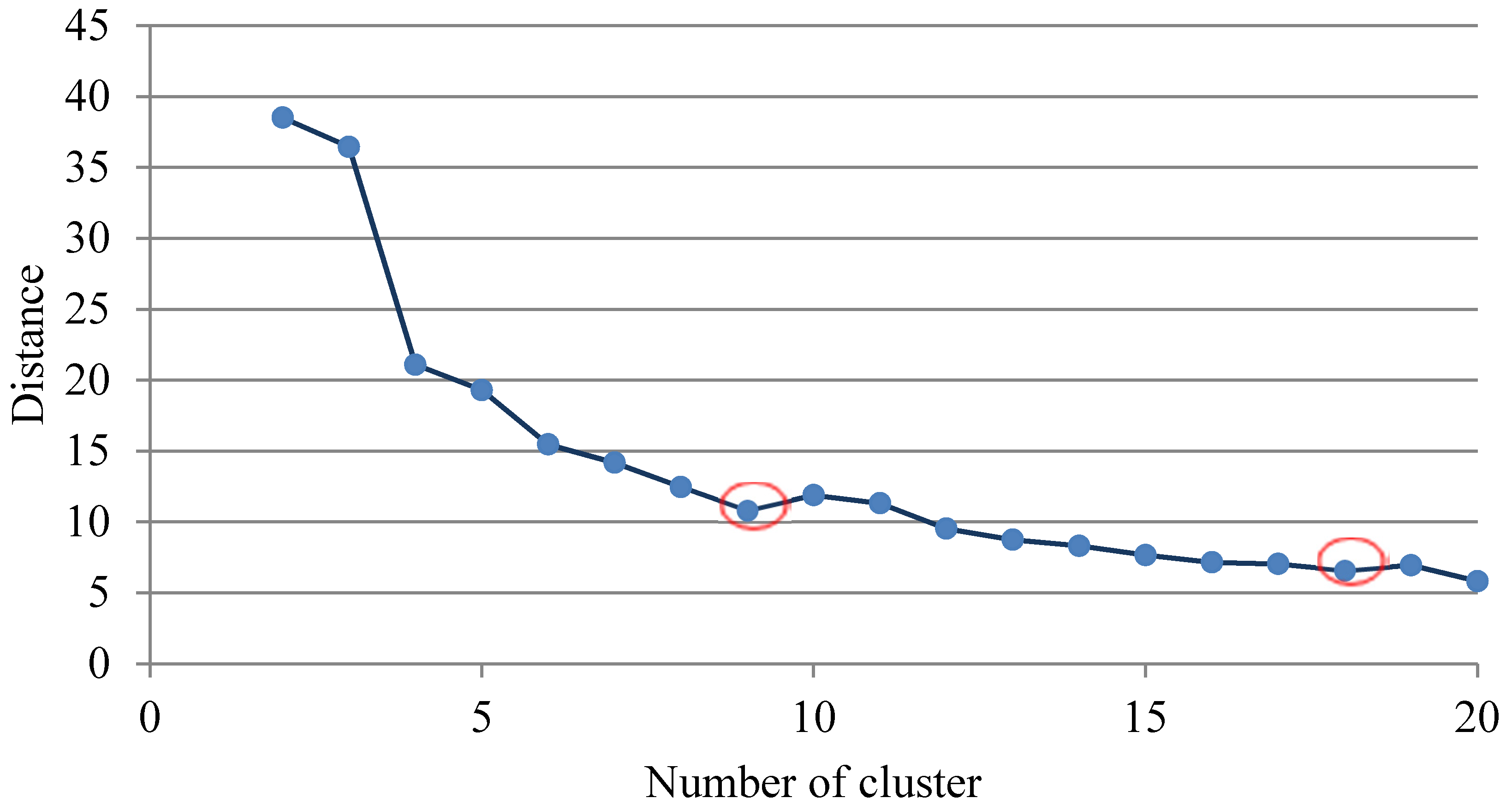
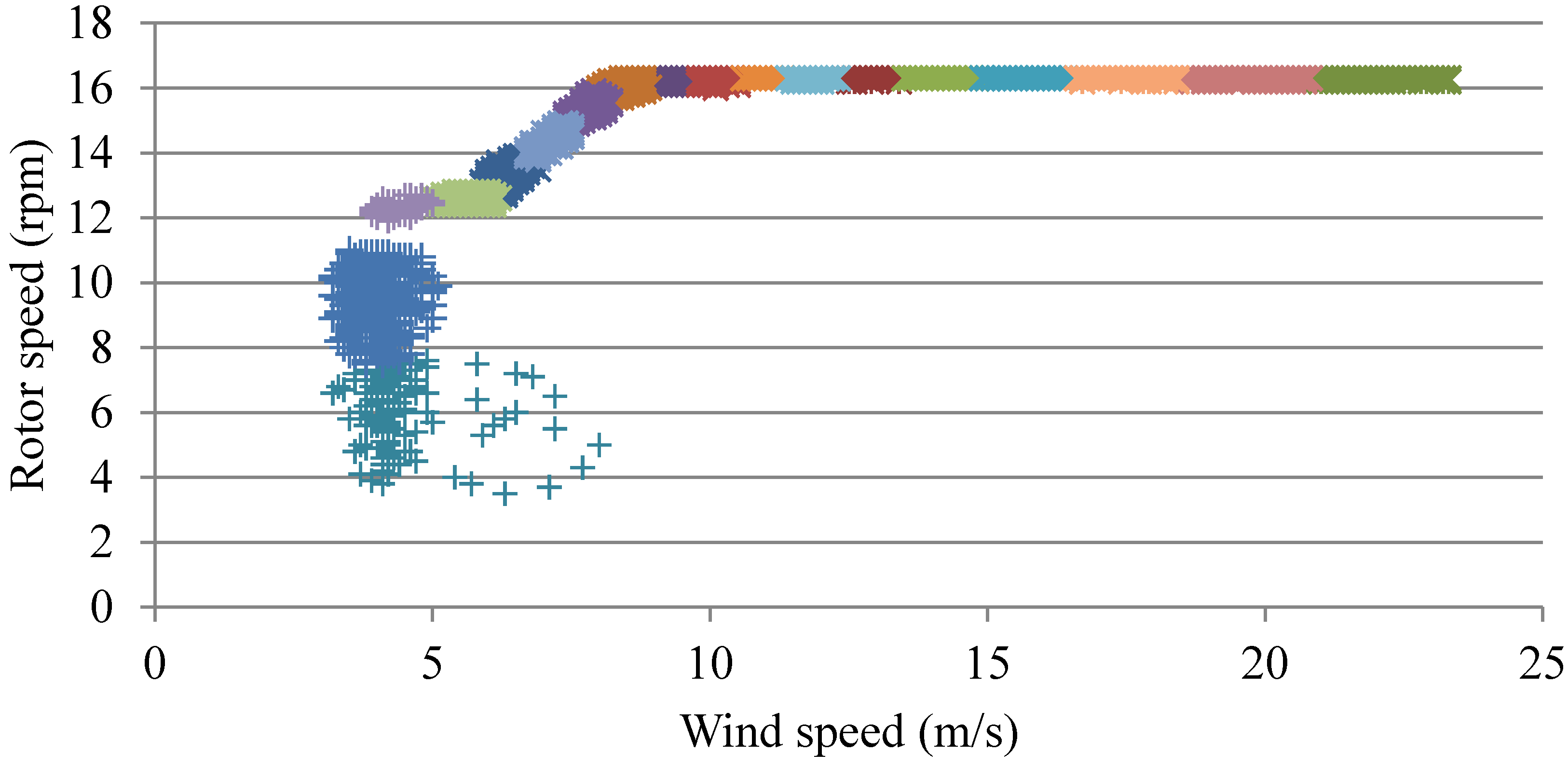
4.1. Clustering for Processing Outliers
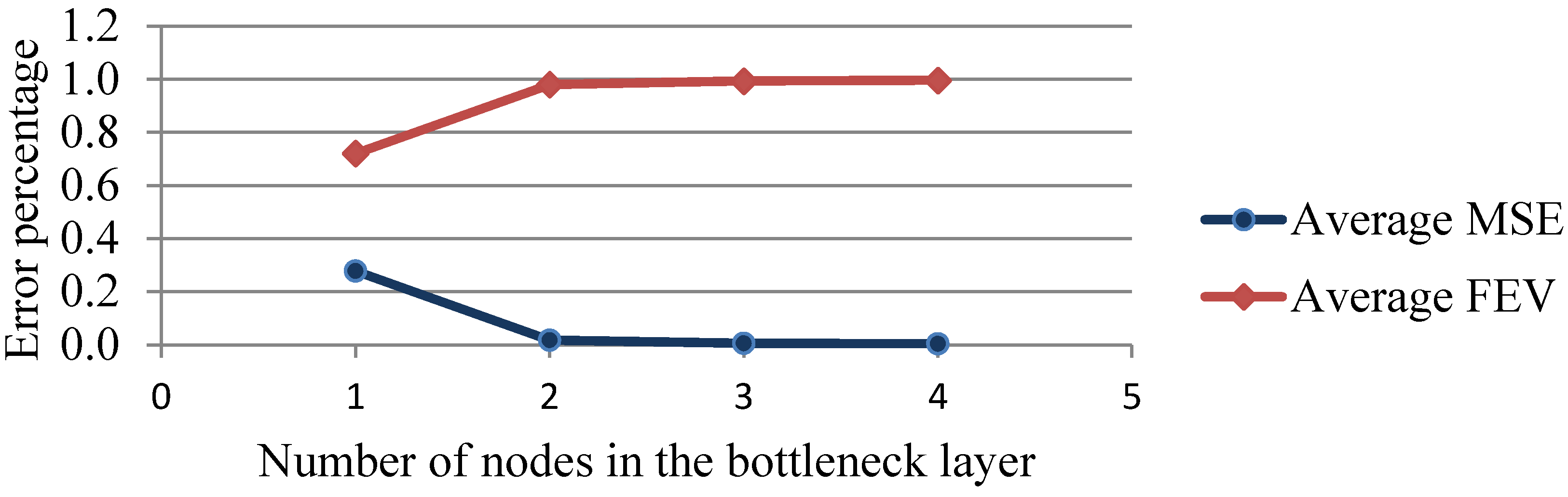
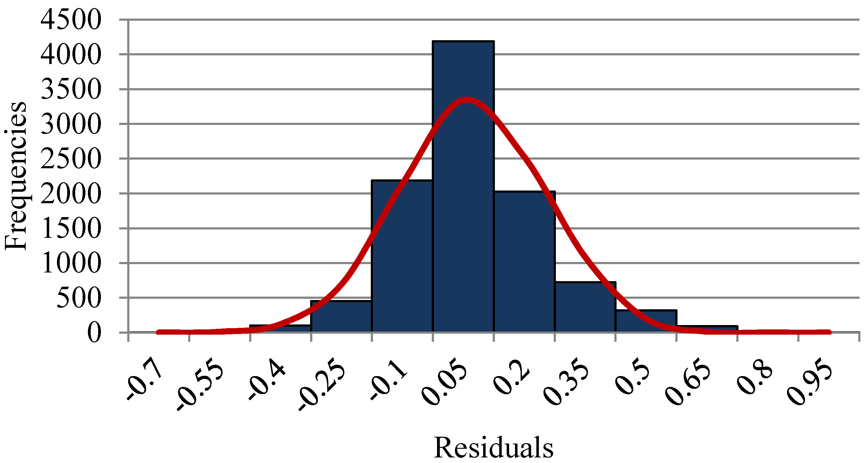
Before clustering, data with missing values or out-of-range values, such as negative power output, are deleted and then normalized. As described earlier, to improve the detection of outliers, we use the k-means clustering algorithm to group each attribute with respect to wind speed into small clusters. In this context, the subscripts i and j of Dij in Equation (1) represent each attribute and wind speed, respectively. To determine the number of k for the k-means clustering algorithm, we measure the difference of distances between consecutive clusters. Using the rotor speed for an example, consider Figure 3, where two “elbow” points are circled in red. The two points suggest that the number k may be 9 or 18. After investigating in more details for the two cases, we found that more normal data are deleted when k is 9 and thus k is determined to be 18. Figure 4 shows the 18 clusters of rotor speed obtained in different colors. Clusters of other attributes are obtained in a similar way. For brevity, we do not show boxplots here but instead provide Figure 5, where both first quartile (Q1) and third quartile (Q3) are smaller after outliers are deleted. Smaller Q1 and Q3 mean that data belonging to the same cluster are more alike. After processing outliers with respect to each independent attribute, we intersect common records and obtain a total of 10,903 for constructing the AANN model.
Figure 3. Relationship between the number of clusters and the distance.
Energies 08 12100 g003
Figure 4. Rotor speed distributions in 18 clusters.
Energies 08 12100 g004
Figure 5. First quartile (Q1) and third quartile (Q3) in 18 clusters of rotor speed.
Energies 08 12100 g005

4.2. Training AANN

It is well known that too many nodes in the hidden layers will produce an over-fitted network, and a specific number of hidden neurons above which the performance of the network begins to degrade [23]. In general, determining the best size of the network is not straightforward and may be found only through a process of trial and error [24]. The process can be performed by generating different types of structures with a different number of nodes and then selects the structure that appears to be more optimal [24]. As a rule of thumb, the number of nodes in the bottleneck layer should be less than that of input layer so that the network does not memorize the input data. To prevent over-fitting and to achieve the desired performance, our methodology for selecting the number of bottleneck nodes is to start the bottleneck layer with one node and the mapping and de-mapping layers are started with a number of nodes greater than the input layer. Various metrics can be considered for measuring the prediction accuracy of the model. The MSE is used for selecting the AANN structure [24,25]. Increasing the number of nodes in the bottleneck layer both improves the network performance (MSE decreases) and increases the FEV [26]. In this paper, we consider both the MSE and FEV simultaneously to determine the best structure of the AANN [6].
Several types of the AANN structures are generated based on the rule just described above and their FEVs and MSEs are shown in Table 3. To determine the best structure, we consider the number of nodes in the bottleneck layer first. To gain insights into the relationship between the FEV and MSE with respect to the number of nodes in the bottleneck layer, we calculate average FEV and MSE of each structure with the same number of bottleneck nodes and provide them in Figure 6. The stopping criteria used for selecting the number of nodes in the bottleneck layer is to observe whether error percentages of the FEV and MSE change marginally. The error percentages of both FEV and MSE are provided in Table 4 and shown in Figure 6 in which the error percentages appear to change marginally when the number of nodes in the bottleneck layer is two, in the sense that two is a reasonable choice for the bottleneck layer. After the number of nodes in the bottleneck layer is selected, the stopping criteria used for selecting the number of nodes in the mapping layer is explained as follows. Recall that the mapping layers are started with a number of nodes greater than the input layer. Consider 8-9-2-9-8, 8-10-2-10-8, and 8-11-2-11-8 in Table 3 as examples. The MSEs of the three structures are 0.0139, 0.0167, and 0.0183, respectively, which show a trend of gradual increase as the number of nodes in the mapping layer increases. This degrading performance indicates that selecting 9 for the mapping layer would avoid over-fitting. On the basis of the explanations just given above and considering MSE and FEV together in Table 3, we select 8-9-2-9-8 as the AANN structure.
Table 3. Training results of the auto-associative neural networks (AANN) structures.
StructureMean Square Error (MSE)Fraction of Explained Variance (FEV)
8-9-1-9-80.32110.6805
8-10-1-10-80.27040.7292
8-11-1-11-80.19110.8015
8-12-1-12-80.32850.6713
8-9-2-9-80.01390.9843
8-10-2-10-80.01670.9809
8-11-2-11-80.01830.9764
8-12-2-12-80.02050.9783
8-9-3-9-80.00630.9938
8-10-3-10-80.00620.9915
8-11-3-11-80.00600.9926
8-12-3-12-80.00500.9946
8-9-4-9-80.00500.9960
8-10-4-10-80.00520.9943
8-11-4-11-80.00220.9974
8-12-4-12-80.00350.9965
Table 4. Error percentages of average MSE and FEV.
Number of Nodes in the Bottleneck LayerAverage MSEAverage FEV
10.27780.7206
20.01730.9800
30.00590.9931
40.00400.9961
Figure 6. Number of nodes in the bottleneck layer versus prediction error percentage.
Energies 08 12100 g006

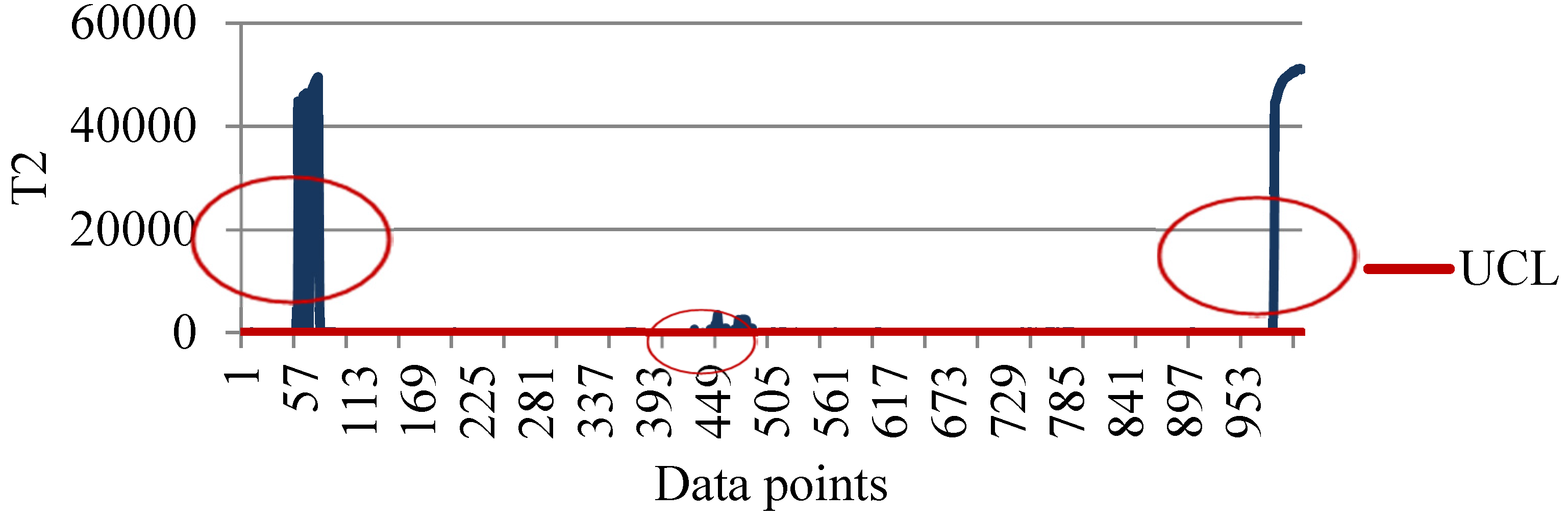
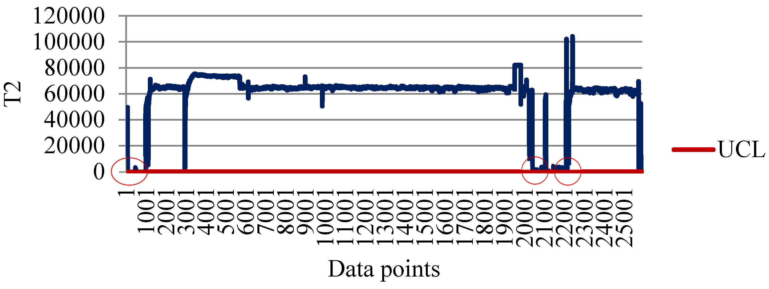
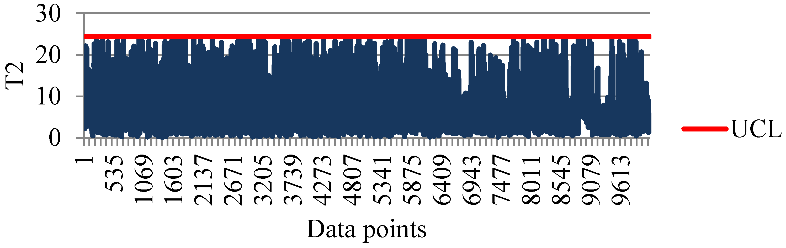
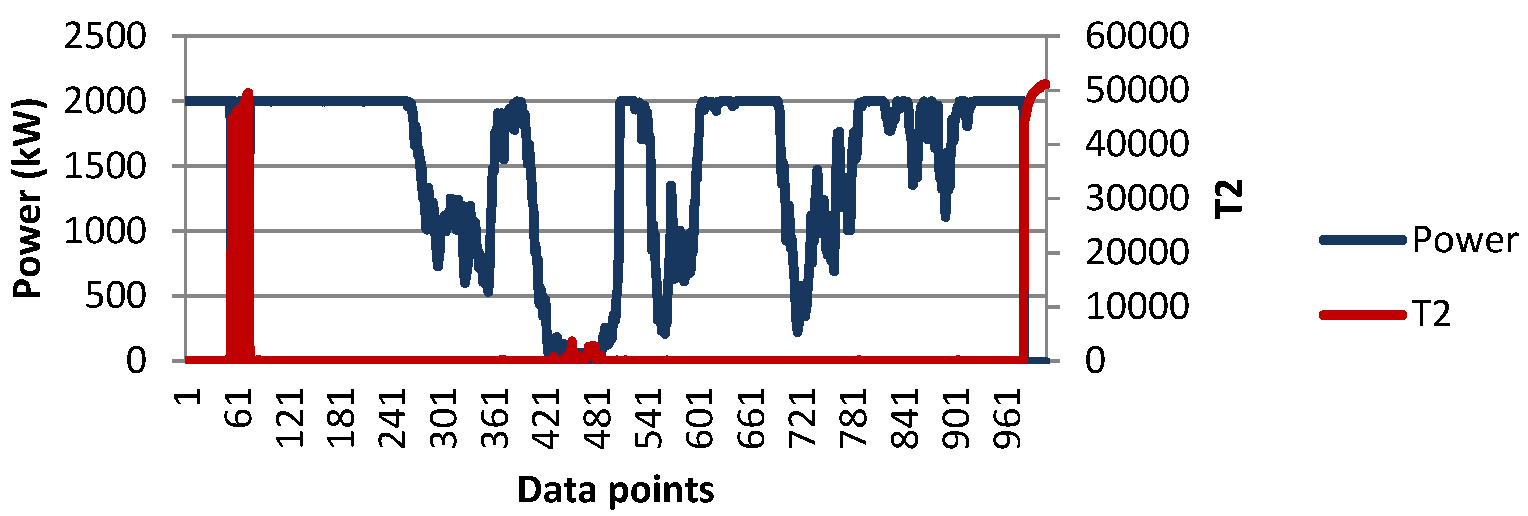
4.3. Constructing Hotelling T2 Control Charts

The Hotelling T2 statistic requires the data to be normally distributed. To deal with the requirement, we follow the residual approach presented in [6,9,10]. In addition, histogram of the residuals is provided to check whether the residuals follow a normal distribution [27]. Take generator bearing temperature for example. Figure 7 shows the standardized residuals of the generator bearing temperature where the normality assumption appears to be justified. Once the residual data calculated from the AANN are available, we use Equation (5) to calculate the UCL, where the value of α is set to 0.001 [4]. Data points larger than T2 statistic are deleted and the training process is repeated until all data points meet the control limits, which produces the UCL of 24.3691 as shown in Figure 8. The number of data points meeting the control limits is 10,135.
Figure 7. Standardized residuals of the generator bearing temperature.
Energies 08 12100 g007
Figure 8. Control limits for residual data points of the generator bearing temperature.
Energies 08 12100 g008

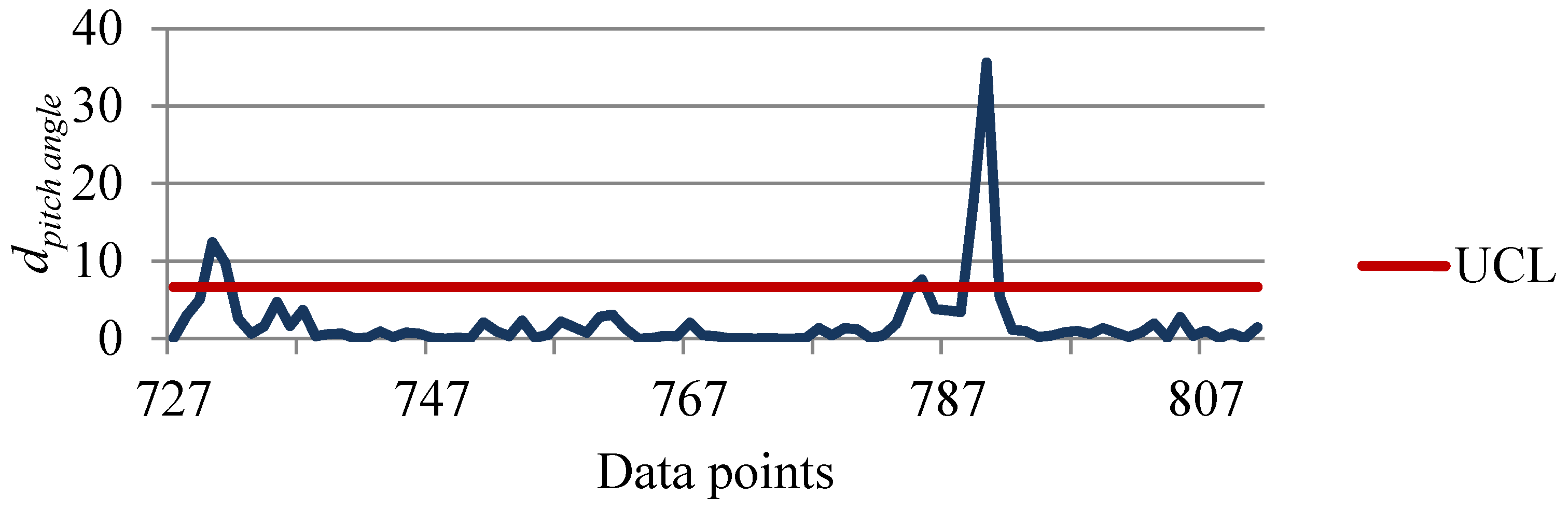
4.4. Detecting Potential Attributes Contributing to Faults

To illustrate how our methodology may help detect the potential attributes, we first provide the power output over 1–20 January 2009 in Figure 9, where power output started to behave abnormally at some time (the 983-th data point) on 7 January 2009 and remained at this status until on 21 January 2009. This motivates us to investigate whether the fault can be detected earlier by monitoring attributes. Now that the fault occurred on 7 January 2009, we analyze the data over 1–7 January 2009 (total 1008 data points) and show the Hotelling T2 control chart in Figure 10, where red circles indicate data points susceptible to various types of anomalies that are determined by the fact that original values of some attributes such as rotor speed change marginally while others considerably. These susceptible data points may reveal important information of attributes contributing to the fault later. We need to point out that susceptible data are not limited to those circled in red. Recall UCL is 24.3691. Due to the scale of vertical axis required to reflect large T2 values of several data points, the data with smaller T2 values are not circled even they are greater than the UCL. In fact, those data points with large T2 values in Figure 10 are mostly the same data points circled in red in Figure 9. Some form of relationship between abnormal power output and large T2 value appears to exist in Figure 11, which leads to an interesting question as to whether simply monitoring the Hotelling T2 statistic can detect faults earlier.
Figure 9. Power output from 1 January 2009 to 20 January 2009.
Energies 08 12100 g009
Figure 10. Control limits for residual data points from 1 January 2009 to 7 January 2009.
Energies 08 12100 g010
Figure 11. Power output versus Hotelling T2 statistic from 1 January 2009 to 7 January 2009.
Energies 08 12100 g011
We continue to focus on a shorter period before the 983-th data point, which is from 5 January 2009 to 7 January 2009 (data points between 600 and 977), and enlarge the Hotelling T2 control chart in Figure 12. Data points between 727 and 811 circled in red in Figure 12 are susceptible. Recall that the Hotelling T2 control charts consider multivariate simultaneously and thus identifying which of the attributes (or which subset of them) contributing to an out-of-control data point is challenging. To cope with the challenge, [5] introduces the method that decomposes the T2 statistic into components reflecting the contribution of each attribute. Therefore, we use Equation (6) to compute relative contribution of each attribute to the overall T2 statistic.
Figure 12. Control limits for residual data points from 5 January 2009 to 7 January 2009.
Energies 08 12100 g012
Consider an attribute, say pitch angle. Relative contribution of the pitch angle, denoted by dpitch angle, to the overall T2 statistic of data points between 727 and 811 is provided in Figure 13. Because the UCL of χ2 with degree of freedom being one is 6.63, dpitch angle greater than 6.63 is susceptible to be anomalous. For example, it can be observed that the 730-th data point in Figure 13 is greater than the UCL, suggesting that pitch angle could be one of attributes contributing to the 730-th overall T2 statistic. Other susceptible attribute at the 730-th data point includes gear oil temperature. Montgomery [5] (p. 511) illustrates a case where the data point would be inside the control limits on both of the univariate charts, yet when the two variables are examined simultaneously, the unusual behavior of the point is fairly obvious. The illustration suggests that both pitch angle and gear oil temperature are attributes more likely than others contributing to the fault later.
Figure 13. Relative contribution of pitch angle to overall T2 between 727 and 811 data points.
Energies 08 12100 g013

4.5. Advantages of Obtained Results Using the Proposed Methodology

On the basis of the preceding study on a short period, we investigate entire year and summarize the results in Table 5. The second column in Table 5 represents the set of attributes in order of occurrence frequency from left to right. For example, ABF represents that pitch angle (A) occurs the most frequent over 1–7 January 2009, followed by gearbox bearing temperature (B) and by power output (F). The third column in Table 5 is determined by the alarm log and includes two types of categories: Either “undetermined” or exact turbine’s component. The undetermined category indicates that the alarm log does not provide sufficient information to identify which component is anomalous. According to Table 5, pitch angle, gear bearing temperature, generator bearing temperature, and generator speed are almost included in each period. This suggests that our methodology has the advantage of detecting a set of susceptible attributes at the same time compared with only one independent attribute is monitored.
Since Table 5 is summarized based on the data of an entire year, Figure 14 shows the graph of the T2 statistic for residual data points ranging only from 1 January 2009 to 30 June 2009 to provide better visual illustration that follows. For example, three red circles in Figure 14 correspond to the first three short periods in Table 5. One can observe that most of the points in Figure 14 have large T2 values that correspond to abnormal power outputs as we mentioned earlier. Although the summary in Table 5 is helpful for early detection, one could wonder whether some false alarms were generated based on the T2 statistical threshold. Due to the imbalance level of the dataset and lack of using the techniques to balance the dataset in this study, identifying true false alarms generated is a difficult task. The difficulty disables us to provide a receiver operating characteristic (ROC) curve that would help summarize the detection accuracy versus false alarm rate.
Table 5. Potential attributes and identified components in 2009.
PeriodPotential AttributesIdentified Component
1–7 January 2009ABFUndetermined
22–27 May 2009ABCDGenerator
1–4 June 2009ABDCGenerator
29 June–8 July 2009ABDCGenerator
18–20 July 2009ABCDGenerator
26–30 July 2009BCDUndetermined
2–10 August 2009ABCDGenerator
31 August–4 September 2009ABCDGenerator
10–14 September 2009BCDAGenerator
28–29 September 2009BCADBlade pitch
15–24 October 2009ABCDUndetermined
10–13 November 2009ABDCBlade pitch
28–30 November 2009ABDCUndetermined
A: pitch angle; B: gear bearing temp.; C: generator bearing temp.; D: generator speed; F: rotor speed.
Figure 14. T2 statistic for residual data points from 1 January 2009 to 30 June 2009.
Energies 08 12100 g014

5. Conclusions

This study proposes a three-phase methodology for detecting a set of attributes of the wind turbine using the SCADA data. We process outlier data by using the k-means clustering method and justify the results by comparing quartiles of boxplots in the first phase. After processing the outliers, we apply the AANN to implement the residual approach in the second phase. We construct the Hotelling T2 quality control charts and detect the set of attributes for data points out of control limits in the third phase. The detection relies on calculating relative contribution of each attribute to the overall Hotelling T2 statistic. Observing power output and T2 statistic simultaneously reveals an interesting question as to whether monitoring the Hotelling T2 statistic can help detect faults earlier.
The study contains several limitations for future work. First, better techniques for attribute selection remain worthwhile to improve research contributions and domain knowledge regarding to the operational ranges of the attributes may be incorporated to improve the detection of outliers. Next, accurately identifying which subset of the attributes contributing to an out-of-control data point remains a challenging issue. Instead of computing relative contribution of each attribute to the overall T2 statistic as used in the paper, alternative approaches to dealing with the challenge is needed. One may consider developing a diagnosis method that uses the contribution values as inputs. Moreover, how to update the model or baseline over time deserves study. Finally, pitch angle is in most cases identified as an attribute contributing to the fault, which may be in large due to turbine’s inability to adjust its pitch angle in time to wind speed. One may consider using moving average windows so that pitch angle can be monitored more closely.

Acknowledgments

This research was supported in part by grant number NSC102-2410-H-167-006-MY2. The authors are grateful to the anonymous reviewers for their constructive comments and suggestions for improving the presentation of the paper. The authors also thank Yu-Liang Chung who kindly provided the data.

Author Contributions

Shih-Wei Yang conducted the research and was supervised by Hsu-Hao Yang and Mei-Ling Huang.

Conflicts of Interest

The authors declare no conflict of interest.

References

  1. Tchakoua, P.; Wamkeue, R.; Ouhrouche, M.; Slaoui-Hasnaoui, F.; Tameghe, T.A.; Ekemb, G. Wind turbine condition monitoring: State-of-the-art review, new trends, and future challenges. Energies 2014, 7, 2595–2630. [Google Scholar]
  2. Kusiak, A.; Zhang, Z.; Verma, A. Prediction, operations, and condition monitoring in wind energy. Energy 2013, 60, 1–12. [Google Scholar] [CrossRef]
  3. Márquez, F.P.G.; Tobias, A.M.; Pérez, J.M.P.; Papaelias, M. Condition monitoring of wind turbines: Techniques and methods. Renew. Energy 2012, 46, 169–178. [Google Scholar] [CrossRef]
  4. Kusiak, A.; Verma, A. Monitoring wind farms with performance curves. IEEE Trans. Sustain. Energy 2013, 4, 192–199. [Google Scholar] [CrossRef]
  5. Montgomery, D.C. Introduction to Statistical Quality Control, 7th ed.; Wiley: New York, NY, USA, 2013. [Google Scholar]
  6. Yang, H.-H.; Huang, M.-L.; Huang, P.-C. Detection of wind turbine faults using a data mining approach. J. Energy Eng. 2015. [Google Scholar] [CrossRef]
  7. Yampikulsakul, N.; Byon, E.; Huang, S.; Sheng, S.; You, M. Condition monitoring of wind power system with nonparametric regression analysis. IEEE Trans. Energy Convers. 2014, 29, 288–299. [Google Scholar]
  8. Marvuglia, A.; Messineo, A. Monitoring of wind farms’ power curves using machine learning techniques. Appl. Energy 2012, 98, 574–583. [Google Scholar] [CrossRef]
  9. Kusiak, A.; Zheng, H.; Song, Z. Models for monitoring wind farm power. Renew. Energy 2009, 34, 583–590. [Google Scholar] [CrossRef]
  10. Kusiak, A.; Zheng, H.; Song, Z. On-line monitoring of power curves. Renew. Energy 2009, 34, 1487–1493. [Google Scholar] [CrossRef]
  11. Kramer, M.A. Nonlinear principal component analysis using auto-associative neural networks. AIChE J. 1991, 37, 233–243. [Google Scholar] [CrossRef]
  12. Bayba, A.J.; Siegel, D.N.; Tom, K. Application of Auto-Associative Neural Networks to Health Monitoring of the CAT 7 Diesel Engine; ARL-TN-0472; U.S. Army Research Laboratory: Adelphi, MD, USA, 2012. [Google Scholar]
  13. Muthuraman, S.; Twiddle, J.; Singh, M.; Connolly, N. Condition monitoring of SSE gas turbines using artificial neural networks. Insight 2012, 54, 436–439. [Google Scholar] [CrossRef]
  14. Uluyol, O.; Parthasarathy, G. Multi-Turbine Associative Model for Wind Turbine Performance Monitoring. In Proceedings of the Annual Conference of the Prognostics and Health Management Society, Minneapolis, MN, USA, 23–27 September 2012.
  15. Kim, K.; Parthasarathy, G.; Uluyol, O.; Foslien, W.; Sheng, S.; Fleming, P. Use of SCADA Data for Failure Detection in Wind Turbines. In Proceedings of the Energy Sustainability Conference and Fuel Cell Conference, Washington, DC, USA, 7–10 August 2011.
  16. Schlechtingen, M.; Santos, I.F. Comparative analysis of neural network and regression based condition monitoring approaches for wind turbine fault detection. Mech. Syst. Signal Process. 2011, 25, 1849–1875. [Google Scholar] [CrossRef]
  17. Worden, K.; Staszewski, W.J.; Hensman, J.J. Natural computing for mechanical systems research: A tutorial overview. Mech. Syst. Signal Process. 2011, 25, 4–111. [Google Scholar] [CrossRef]
  18. Santos, P.; Villa, L.F.; Reñones, A.; Bustillo, A.; Maudes, J. An SVM-based solution for fault detection in wind turbines. Sensors 2015, 15, 5627–5648. [Google Scholar] [CrossRef] [PubMed]
  19. Kusiak, A.; Zhang, Z. Short-horizon prediction of wind power: A data-driven approach. IEEE Trans. Energy Convers. 2010, 25, 1112–1122. [Google Scholar] [CrossRef]
  20. Zaher, A.; McArthur, S.D.J.; Infield, D.G.; Patel, Y. Online wind turbine fault detection through automated SCADA data analysis. Wind Energy 2009, 12, 574–593. [Google Scholar] [CrossRef]
  21. Schlechtingen, M.; Santos, I.F.; Achiche, S. Wind turbine condition monitoring based on SCADA data using normal behavior models. Part 1: System description. Appl. Soft Comput. 2013, 13, 259–270. [Google Scholar]
  22. Han, J.; Kamber, M.; Pei, J. Data Mining: Concepts and Techniques, 3th ed.; Morgan Kaufmann Publishers: Waltham, MA, USA, 2011. [Google Scholar]
  23. Kerschen, G.; Golinval, J.-C. Feature extraction using auto-associative neural networks. Smart Mater. Struct. 2004, 13, 211–219. [Google Scholar] [CrossRef]
  24. Sanz, J.; Perera, R.; Huerta, C. Fault diagnosis of rotating machinery based on auto-associative neural networks and wavelet transforms. J. Sound Vib. 2007, 302, 981–999. [Google Scholar] [CrossRef]
  25. Dervilis, N.; Choi, M.; Taylor, S.G.; Barthorpe, R.J.; Park, G.; Farrar, C.R.; Worden, K. On damage diagnosis for a wind turbine blade using pattern recognition. J. Sound Vib. 2014, 333, 1833–1850. [Google Scholar] [CrossRef]
  26. Bulunga, M.L. Change-point Detection in Dynamical Systems Using Auto-Associative Neural Networks. Master’s Thesis, Faculty of Engineering, Stellenbosch University, Stellenbosch, South Africa, March 2012. [Google Scholar]
  27. Harrou, F.; Nounou, M.N.; Nounou, H.N.; Madakyaru, M. Statistical fault detection using PCA-based GLR hypothesis testing. J. Loss Prevent. Proc. 2013, 26, 129–139. [Google Scholar] [CrossRef]

