Article

A Novel Design Method for Optimizing an Indirect Forced Circulation Solar Water Heating System Based on Life Cycle Cost Using a Genetic Algorithm

Urban Development Institute, Incheon National University, Incheon 406-772, Korea
Energies 2015, 8(10), 11592-11617; https://doi.org/10.3390/en81011592
Submission received: 24 August 2015 / Revised: 3 October 2015 / Accepted: 11 October 2015 / Published: 16 October 2015
(This article belongs to the Special Issue Solar Heating & Cooling)

Abstract

:
To maximize the energy performance and economic benefits of solar water heating (SWH) systems, the installation and operation-related design variables as well as those related to capacity must be optimized. This paper presents a novel design method for simultaneously optimizing the various design variables of an indirect forced-circulation SWH system that is based on the life cycle cost and uses a genetic algorithm. The effectiveness of the proposed method is assessed by evaluating the long-term performance corresponding to four cases, which are optimized using different annual solar fractions and sets of the design variables. When the installation and operation-related design variables were taken into consideration, it resulted in an efficient and economic design and an extra cost reduction of 3.2%–6.1% over when only the capacity-related design variables were considered. In addition, the results of parametric studies show that the slope and mass flow rate of the collector have a significant impact on the energy and economic performances of SWH systems. In contrast, the mass flow rate in the secondary circuit and the differences in the temperatures of the upper and lower dead bands of the differential controller have a smaller impact.

1. Introduction

Solar water heating (SWH) systems have been recognized as the most promising alternative energy systems for heating because they reduce the consumption of fossil fuels and the emission of greenhouse gases. However, their energy and economic performances vary considerably depending on the weather and load conditions. Therefore, SWH systems must be designed properly to ensure that the benefits to the user are maximized.
Over the last few decades, a number of studies have focused on optimizing the designs of SWH systems. The design methods reported thus far can be broadly classified into correlation-based methods such as the ϕ method [1], ϕ ¯ method [2], f -chart method [3], and ϕ ¯ , f -chart method [4] and simulation-based methods such as transient system simulation (TRNSYS) [5] and pre-design and optimization tool for solar heating systems with seasonal storage (SOLCHIPS) [6]. The correlation-based methods were developed on the basis of the results of a large number of detailed simulation studies. The results of these simulations were correlated in terms of easily calculated dimensionless variables, or were presented as the integrated collector performance in the form of functions of the collector characteristics, location, and orientation. It was assumed that the inlet temperature of the fluid remained constant [7]. Therefore, the methods belonging to the former category are limited in their usefulness when the meteorological data and the design parameters of the SWH system are different from those used in developing its correlations [8]. On the other hand, the methods belonging to the latter category involve high computation times.
Therefore, in recent years, efforts have been made to use new optimization methods such as linear and nonlinear optimization methods and evolutionary algorithms to improve the design of SWH systems. Loomans et al. [9] presented a method to optimize the design variables such as the types and numbers of collectors, storage tanks, and heat exchangers by minimizing the payback period using a genetic algorithm (GA). Krause et al. [10] optimized the design parameters of an existing large solar thermal system by using a GA to improve its performance. Kalogirou [11] optimized the sizes of the collector area and storage tank for maximizing life-cycle savings by using both artificial neural networks and a GA. Bornatico et al. [12] presented a method for finding the optimal sizes of the collector, storage tank, and auxiliary heater using particle swarm optimization. Yan et al. [8] presented a simplified design method for optimizing the collector area and storage tank volume based on a life cycle energy analysis. Kim et al. [13] optimized the collector area and storage tank volume of an existing active-indirect SWH plant by minimizing the capital payback period using a micro GA. Kulkarni et al. [14] proposed the “design space methodology” for determining the size of the collector as well as the storage for a given solar fraction by minimizing the annualized life cycle cost (LCC). Atia et al. [15] optimized the size of a forced circulation SWH system for an aquaculture system using a GA. Choi et al. [16] presented a design method to optimize the size of the SWH system using a GA.
However, most of these studies were focused on determining the sizes of the main components of an SWH system, such as the collector, storage tank, heat exchanger, and auxiliary heater. Although these components have a significant effect on the energy and economic performances of SWH systems, other design variables such as the collector slope, flow rates of the liquid on the source and load sides, and operating conditions of the differential temperature controller must also be considered. In addition, these design parameters influence each other and are all related to the overall system performance to some extent. Therefore, in order to ensure good performance and to maximize the economic benefits, all of these parameters should be optimized as comprehensively as possible. Furthermore, most previous studies were aimed at optimizing a particular SWH system, that is, a single model selected beforehand by researchers. In these studies, the appropriate sizes of the main components were determined on the basis of the quantitative changes corresponding to a particular device. However, many models are available for each component in the marketplace, and they all have different technical and economic characteristics. Thus, their use would lead to variations in the energy and economic performances of the system.
Therefore, this paper presents a novel design method for simultaneously optimizing the various design variables of a forced circulation SWH system. The design variables considered in this study included the types and numbers of collector and auxiliary heaters; the types of storage tanks, heat exchangers; the collector slope; flow rates of the liquid on the source and load sides; and the operating conditions of the differential temperature control. In addition, the sizes of the main components are optimized for a wide range of device types available in the marketplace. A GA is used to optimize the design variables by minimizing the LCC of an SWH system. Further, this study assesses the effectiveness of the proposed optimization method for an indirect forced circulation SWH system by analyzing four cases, which are simulated using different solar fractions and sets of design variables. The effects of the operation-related design variables on the energy and economic performances of the SWH system are also evaluated.

2. Mathematical Models of SWH System

Indirect forced circulation SWH systems are used in many countries with cold climates. However, studies on the optimization of these systems are few, in contrast to those on the other SWH systems such as thermosiphon SWH systems. Therefore, in this study, an indirect forced circulation SWH system that is suitable for water heating in cold regions, including in South Korea, was optimized. Figure 1 shows the standard system configuration for water heating only. It consists of flat-plate solar collectors, an external heat exchanger, a storage tank, and auxiliary heaters. In addition, this general configuration is also being employed and improved upon in other applications of solar energy systems, such as photovoltaic/thermal systems [17,18,19] and solar-driven heat and power systems [20]. The primary fluid, i.e., antifreeze fluid, circulates between the collectors and the hot side of an external heat exchanger. It transports the collected solar energy to water that circulates between a storage tank and the cold side of an external heat exchanger. When hot water is demanded, the hot water from the storage tank passes through the auxiliary heaters. If the temperature of the storage tank is below the desired set temperature, the auxiliary heaters are switched on.
Figure 1. Schematic diagram of an indirect forced circulation solar water heating (SWH) system.
Energies 08 11592 g001

2.1. Solar Radiation

According to the isotropic diffuse model, the total solar radiation incident on a tilted surface can be determined using the following equation [7]:
I T = I b R b + I d ( 1 + c o s β c o l l 2 ) + I ρ g ( 1 c o s β c o l l 2 )
where I T is the hourly total solar radiation incident on the tilted collector array (W/m2); I b , I d , and I are the hourly beam, diffuse, and global radiation incident on a horizontal surface, respectively (W/m2); R b is the ratio of the beam radiation incident on the tilted surface to that on a horizontal surface; ρ g is the ground reflectance (0.2 for non-snow surfaces); and β c o l l is the slope of the collector array (degrees).

2.2. Flat Plate Solar Collector

The useful heat gain of identical solar collectors in series is given by the following equation [7]:
q u = A c o l l N c o l l , s [ F R ( τ α ) I T F R U L ( T h o T a ) ] +
where A c o l l is the gross area of a single collector module (m2); N c o l l ,   s is the number of identical collectors in series; F R ( τ α ) and F R U L are the intercept and slope of the efficiency curve of the identical collector modules in series, respectively; T h o is the hot stream outlet temperature of the heat exchanger (°C); T a is the outdoor dry-bulb temperature (°C); and the + sign indicates that hot water from the collector array circulates the hot stream only when the useful solar heat gain becomes positive.
For identical collector modules in series, the intercept and slope of the efficiency curve can be estimated using the following equations [7]:
F R ( τ α ) = F R 1 ( τ α ) 1 [ 1 ( 1 A c o l l F R 1 ( τ α ) 1 A c o l l m c o l l , u C p , c ) N c o l l , s N c o l l , s A c o l l F R 1 ( τ α ) 1 A c o l l m c o l l , u C p , c ]
F R U L = F R 1 U L 1 [ 1 ( 1 A c o l l F R 1 ( τ α ) 1 A c o l l m c o l l , u C p , c ) N c o l l , s N c o l l , s A c o l l F R 1 ( τ α ) 1 A c o l l m c o l l , u C p , c ]
where F R 1 ( τ α ) 1 and F R 1 U L 1 are the intercept and slope of the efficiency curve of a single collector, respectively; m c o l l ,   u is the mass flow rate per unit area of the collector fluid (kg/s·m2); and c p , c is the specific heat capacity of the collector fluid (J/kg·°C).

2.3. Differential Temperature Controller

In the optimization method used, the forced circulation SWH system is controlled using a differential temperature controller on an hourly basis. This common control requires two temperatures, namely, that of the bottom of the storage tank as the lower input temperature and that of the exit of a collector as the upper input temperature. It is also necessary to set up dead band conditions to prevent the on/off cycling of the circulation pump. If the controller was previously on, the control function is expressed as follows:
γ o = { 1 ,   γ i = 1   a n d   Δ T o f f T H T L 0 ,   γ i = 1   a n d   Δ T o f f > T H T L
Conversely, if the controller was previously off, the control function is expressed as follows:
γ o = { 1 ,   γ i = 0   a n d   Δ T o n T H T L 0 ,   γ i = 0   a n d   Δ T o n > T H T L
where γ i and γ o are the input and output control functions, respectively; T H and T L are the upper and lower input temperature, respectively (°C); and Δ T o n and Δ T o f f are the temperature differences of the upper and lower dead bands, respectively (°C).

2.4. Heat Exchanger

To calculate the performance of the heat exchanger in an SWH system, the effectiveness ( ε )-number of transfer units (NTU) method is used. The ε -NTU method uses three dimensionless parameters: the heat-exchanger effectiveness ( ε ), the number of exchanger heat transfer units (NTU), and the capacity rate ratio ( c r ). For a given counter-flow heat exchanger, these three parameters can generally be expressed as follows [7]:
ε = { 1 e x p [ N T U ( 1 c r ) ] 1 c r e x p [ N T U ( 1 c r ) ] ,   c r 1 N T U N T U + 1 ,   c r = 1
c r = C h e x , m i n C h e x , m a x
N T U = U A h e x C h e x , m i n
where C h e x , m i n and C h e x , m a x are the minimum and maximum hot-fluid capacity rate ( C h e x , h ) and cold-fluid capacity rate ( C h e x , c ), respectively; and U A h e x is the overall heat transfer coefficient-area product of the heat exchanger (W/°C).
The capacity rate of the fluid on the hot side of the heat exchanger is given as follows:
C h e x , h = A c o l l m c o l l , u N c o l l , p c p , c
where N c o l l , p is the number of parallel connections in the collector array.
The capacity rate of the fluid on the cold side of the heat exchanger is given as follows:
C h e x , c = m h e x , c c p , w
where m h e x , c is the mass flow rate on the cold side of the heat exchanger (kg/s); and c p , w is the specific heat capacity of water (J/kg·°C).
Therefore, the heat transfer rate, hot-stream outlet temperature, and cold-stream outlet temperature can be determined as follows:
q h e x = { ε C h e x , h ( T h i T c i ) γ o ,   C h e x , m i n = C h e x , h ε C h e x , c ( T h i T c i ) γ o ,   C h e x , m i n = C h e x , c
T h o = T h i q h e x C h e x , h
T c o = T c i + q h e x C h e x , c
where T h i is the hot stream inlet temperature of the heat exchanger (°C), and T c i and T c o are the cold stream inlet and outlet temperatures of the heat exchanger, respectively (°C).

2.5. Storage Tank

At any instant of time, the energy balance of a well-mixed storage tank can be described as follows [14]:
( ρ w c p , w V s ) d T s d t = q h e x q L s q l q d
where ρ w is the density of water (kg/m3); V s is the volume of the storage tank (m3); and q l , q d , and q L s are the heat loss of the storage tank (W), heat discharged to prevent the overheating of the storage tank (W), and solar energy extracted from the storage tank (W), respectively.
To ensure that the hot-water temperature and flow rate are at the desired levels, the water discharged from the storage tank is mixed with make-up water. By considering the mass and energy balance at the mixing junction, the flow rate of the water drawn from the tank can be expressed as follows:
m s = { m l ( T l T m T s T m ) ,   T s > T l m l ,   T s T l
where m s is the mass flow rate from the storage tank to the load (kg/s); m l , the mass flow rate of the desired hot water load (kg/s); T l , the desired hot water temperature; and T m , the make-up water temperature (°C).
Therefore, the solar energy supplied from the storage tank to the load ( q L s ) can be estimated as follows:
q L s = m s c p , w ( T s T m )
Meanwhile, the loss of energy from the storage tank ( q l ) to the surroundings can be expressed as follows:
q l = U s A s ( T s T a m b )
where U s and A s are the heat loss coefficient (W/m2·°C) and the surface area (m2) of the storage tank, respectively, and T a m b is the ambient temperature (°C).
In this study, an optimization method was developed to design an SWH system for low-temperature applications (lower than 100 °C), such as a residential hot water system. Therefore, if the storage tank temperature is greater than the maximum allowable temperature ( T s , m a x ), the surplus heat is discharged to prevent the overheating of the storage tank. The discharged flow rate and heat can be calculated as follows:
m d = { ρ w V s ( T s T s , m a x ) ( T s T m ) ,   T s > T s , m a x 0 ,   T s T s , m a x
q d = { m d c p , w ( T s T s , m a x ) ,   T s > T s , m a x 0 ,   T s T s , m a x
The SWH system parameters from Equation (2) to Equation (20) are evaluated based on the initial temperature of the storage tank at any time step. The final storage tank temperature at the end of any time step must be known because it will be the initial temperature for the next time step. The final storage tank temperature can be estimated as follows:
T s , f = T s + ( q h e x q L s q l q d ) 3 , 600 ρ w c p , w V s Δ t
where T s , f is the final storage tank temperature at the end of any time step (°C).

2.6. Auxiliary Heater

If the storage tank temperature is less than the desired hot water temperature, the water discharged from the tank is heated by auxiliary heaters. The energy for auxiliary heating can be calculated as follows:
q a u x = { 0 ,   T s > T l m l c p , w ( T l T s ) ,   T s T l
The gas consumption of the auxiliary heaters is calculated using a simple model based on their overall efficiency and part load ratio, which is determined by the device capacity and the energy required to meet the load, as shown below [21]:
P L R a u x = q a u x q a u x , t o t a l
E I R ( P L R a u x ) = a + b P L R a u x + c P L R a u x 2 + d P L R a u x 3
F L N G = q a u x E I R ( P L R a u x ) P L R a u x η a u x Q L N G , L H V
where P L R a u x is the part load ratio of the auxiliary heaters at each time step; q a u x ,   t o t a l is the heating capacity of the auxiliary heaters (W); E I R ( P L R a u x ) is the energy input ratio of the auxiliary heater; a, b, c, and d are the coefficients for the energy input ratio; F L N G is the hourly liquid natural gas (LNG) consumption (m3); η a u x is the overall efficiency of the auxiliary heaters; and Q L N G ,   L H V is the fuel lower heating value of LNG (W/m3).

2.7. Circulation Pump

An indirect forced circulation SWH system requires two circulation pumps, which are turned on or off by the differential temperature controller on the hot and cold sides of the heat exchanger. The electricity consumption of the circulation pumps is calculated using the simple model shown below:
F E L E = γ o m f l u i d g H p η p η m
where F E L E is the electricity consumption of the circulation pump (W); m f l u i d , is the flow rate of the fluid passing through the pump (kg/s); g is the acceleration due to gravity (m/s2); H p is the pump head (m); η p is the pump efficiency; and η m is the motor efficiency.

2.8. Energy Performance of an SWH System

When evaluating the energy performance of an SWH system on a monthly or yearly basis, the accumulated performance for a time horizon must be known. The most widely used performance indicators of SWH systems include the solar fraction of the SWH system, efficiency of the collector array, and efficiency of the solar system [8,13,14,15]. These are described by Equations (27)–(29), respectively.
F S = 1 0 t ( q a u x q L ) d t
η c o l l = 0 t ( q u ) d t / 0 t A c o l l N c o l l ( I T ) d t
η s y s = 0 t ( q L s ) d t / 0 t A c o l l N c o l l ( I T ) d t
where q L is the hourly hot water load; N c o l l is the number of solar collectors; and F S , η c o l l , and η s y s are the solar fraction, efficiency of the collector array, and efficiency of the solar system over the given time horizon, respectively.

3. Optimization Method of SWH System

3.1. Decision Variable

In this study, an optimization method was developed to determine the optimal capacities, and installation and operating conditions for a forced circulation SWH system. The capacities of the main components such as the solar collectors, storage tank, heat exchanger, and auxiliary heaters were computed on the basis of their unit capacity and quantity. The capacity units of a solar collector, storage tank, heat exchanger, and auxiliary heater are the area of the collector module (m2), the tank volume (m3), the overall heat transfer coefficient-area product of the heat exchanger (W/°C), and the rated heating rate (kW), respectively. The number of storage tanks and heat exchangers was fixed as one, because this is the most common configuration for indirect forced circulation SWH systems in South Korea. In this study, the slope of the collector array, the mass flow rates on the hot and cold sides of the heat exchanger, and the differences in the temperatures of upper and lower dead bands as design parameters were also considered. Therefore, the design of the SWH system was expressed as a decision vector composed of eleven integer variables, as shown below:
x = ( T c o l l , N c o l l , T h e x ,   T t a n k , T a u x , N a u x , β c o l l ,   m c o l l , u ,   m h e x , c ,   Δ T o n ,   Δ T o f f ) T
where T c o l l is the type of the solar collector; T h e x , the type of the heat exchanger; T t a n k , the type of storage tank; T a u x , the type of the auxiliary heater; and N a u x , the number of auxiliary heaters.

3.2. Objective Function

This optimization method was employed to determine the optimal design for an SWH system by minimizing the LCC, which includes all the costs incurred over the lifetime of the system. The objective function can be expressed as follows [16]:
C L C C = C I + C M + C R + C E C S
where C I , C M , C R , C E , and C S represent the initial, maintenance, replacement, energy, and subsidy costs respectively.
The initial cost is related to the direct purchase cost of the main components and the supplementary cost as follows:
C I = ( C c o l l , j N c o l l + C h e x , j + C t a n k , j + C a u x , j N a u x ) ( 1 + R I )
where C c o l l , j , C h e x , j , C t a n k , j , and C a u x , j are the purchase prices of the j th solar collector, heat exchanger, storage tank, and auxiliary heater, respectively, and R I is the percentage of the supplementary cost with respect to the direct purchase cost.
The maintenance cost is calculated as a percentage of the initial cost of the SWH system as follows:
C M = C I R M [ ( 1 + i ) n p 1 i ( 1 + i ) n p ]
where R M is a percentage of the annual maintenance cost with respect to the initial cost; n p , the planning period; and i , the real discount rate.
Replacement costs are incurred depending on each component’s lifetime during the planning period as follows:
C R , c = n r , c = 1 n r , c { C I , c [ 1 ( 1 + i ) ( n l , c n r , c ) ] }
where C R , c and C I , c are the replacement and initial costs of each component, respectively; n l , c is the lifetime of each component; and n r , c is the number of times each component is replaced.
The energy cost is computed by applying the electricity and LNG price escalation rates as follows:
C E = U P A E L E * t = 1 8 , 760 C E L E ( t ) F E L E ( t ) + U P A L N G * t = 1 8 , 760 C L N G ( t ) F L N G ( t )
U P A f u e l * = ( 1 + e f u e l 1 + i ) [ ( 1 + e f u e l 1 + i ) n p 1 ] ( 1 + e f u e l 1 + i ) 1
where U P A E L E * and U P A L N G * are the uniform present value factor adjusted to reflect the electricity and LNG price escalation rates, respectively; C E L E and C L N G are the hourly electricity cost [KRW/kW·h] and hourly LNG cost [KRW/m3] for the SWH system, respectively; F E L E and F L N G are the hourly electricity consumption [kW·h] and hourly LNG consumption [m3], respectively; and e f u e l is the fuel price escalation rate.
It is assumed that part of the initial cost is supported by the government, depending on the regulations regarding the installation of renewable energy systems. According to the total gross area of the collector modules, the subsidy cost can be calculated as follows:
C S = { C I R S ,   A R , m a x > A c o l l , j N c o l l , j [ C c o l l , j f l o o r ( A R , m a x A c o l l , j ) + C h e x , j + C t a n k , j + C a u x , j N a u x , j ] ( 1 + R I ) R S ,   A R , m a x A c o l l , j N c o l l , j
where A c o l l , j is the gross area of the j th solar collector; A R , m a x , the maximum capacity available to receive the subsidy cost (m2); and R S , the percentage of the subsidy cost with respect to the initial cost (%).

3.3. Constraint Conditions

In the proposed optimization method, any decision vector should be subject to the following constraint conditions.
(a)
The limits of T c o l l , T h e x , T t a n k , and T a u x are set automatically to the number of types of each component in the inputted data tables.
(b)
The limits of N c o l l and N a u x are not set because any decision vector should be subject to the inequality constraints (c) and (e), in order for the solution to be feasible.
(c)
Energy balance:
q L , p e a k q a u x , j N a u x
(d)
Solar fraction (penetration of solar energy):
F S , m i n ( 1 Q a u x , y e a r Q L , y e a r ) × 100 F S , m a x
(e)
Available space to install collector array:
N c o l l W c o l l , j H c o l l , j [ c o s ( β ) + s i n ( β c o l l ) t a n ( α s , w ) ] A c o l l , m a x
(f)
Slope of collector array:
0 β c o l l 90
(g)
Flow rate on hot and cold sides of heat exchanger:
0.005 m c o l l , u 0.025
0.5 A c o l l , j m c o l l , u N c , p m h e x , c 2.0 A c o l l , j m c o l l , u N c , p
(h)
NTU of heat exchanger:
N T U 4
(i)
Control condition of differential temperature controller:
7 Δ T O N 12
1 Δ T O F F 6
where q L , p e a k is the peak hot water load (W); q a u x , j is the heating capacity of the j th auxiliary heater (W); Q L , y e a r is the annual hot water load (W·h); Q a u x , y e a r is the amount of heating energy provided annually by the auxiliary heaters (W·h); F S , m i n and F S , m a x are the minimum and maximum solar fractions, respectively (%); W c o l l , j and H c o l l , j are the width and height of the j th solar collector, respectively (m); α s , w is the meridian altitude in winter (degrees); and A c o l l , m a x is the space available to install the solar collectors (m2).

3.4. Use of GA to Optimize SWH Systems

GAs are effective and popular metaheuristic optimization methods that are well suited to designing energy systems. In this study, a real-coded GA [22] was used to optimize the SWH system. The GA parameters used in this study were as follows: number of generations = 3000, population size = 50, crossover probability = 0.9, and mutation probability = 0.3. The proposed optimization algorithm was implemented using a hierarchical structure, as shown in Figure 2. The top-down instructions were as follows:
Step 1: Read input data
The input data for the proposed method includes the hourly solar radiation and outdoor temperature data, hourly load profiles, and technical specifications of the main components as listed in the appendix at the end of this paper, as well as the data to calculate the objective function and evaluate the constraint conditions.
Step 2: Initialization
During the second step, the GA parameters such as the population size, number of generations ( N g , s e t ), crossover probability, and mutation probability are specified. Then, a random set of possible individuals corresponding to the decision vectors is generated. The individuals that violate the constraints as described in Section 3.3 are removed, and probable individuals are generated randomly.
Step 3: Perform energy simulation
All the individuals in the population are simulated on an hourly basis using mathematical models as described in Section 2 as well as the input data loaded in Step 1.
Step 4: Evaluate objective function
The LCC of each individual is calculated based on the cost functions described in Section 3.2 using the simulation results obtained in Step 3 and the economic data inputted in Step 1. Then, all individuals are sorted on the basis of the values of the objective function.
Step 5: Check termination condition
If the number of iterations reaches the maximum number of generations set in Step 2, the process is terminated, and the minimum LCC at the late generation is obtained as the solution. This is the optimal design for the SWH system. Otherwise, the individuals go through genetic operations such as selection, crossover, and mutation, and the algorithm is repeated from Step 3 onwards.
Figure 2. Flowchart of the proposed optimization algorithm.
Energies 08 11592 g002

4. Case Study and Discussion

4.1. Case Study Description and Parameters

The effectiveness of the suggested optimization method was assessed by analyzing four case studies, each of which was simulated with different sets of design variables and solar fractions. Case1-D and Case1-A were optimized at an annual solar fraction of 40%, which is representative of a wide range of solar applications in South Korea. Case2-D and Case2-A were optimized at an annual solar fraction of 80%, in order to analyze the optimization characteristics of an SWH system with a high solar fraction. Furthermore, to evaluate the variation in the optimization designs of the SWH system with the design variables, the case studies were optimized with respect to the set of the different design variables. For Case1-D and Case2-D, six design variables— T c o l l , N c o l l , T h e x , T t a n k , T a u x , and N a u x —were optimized. These only determine the size of the main components of an SWH system in a manner similar to the case studies taken from the literature. In Case1-A and Case2-A, 11 design integer variables were optimized, as shown in Equation (30). These included operation-related variables as well as capacity-related variables. For Case1-D and Case2-D, the operation-related variables were β c o l l = 35°, m c o l l , u = the mass flow rate per unit collector area under the tested conditions, m h e x , c = A c o l l m c o l l , u N c o l l , p , Δ T o n = 8 °C, and Δ T o f f = 2 °C.
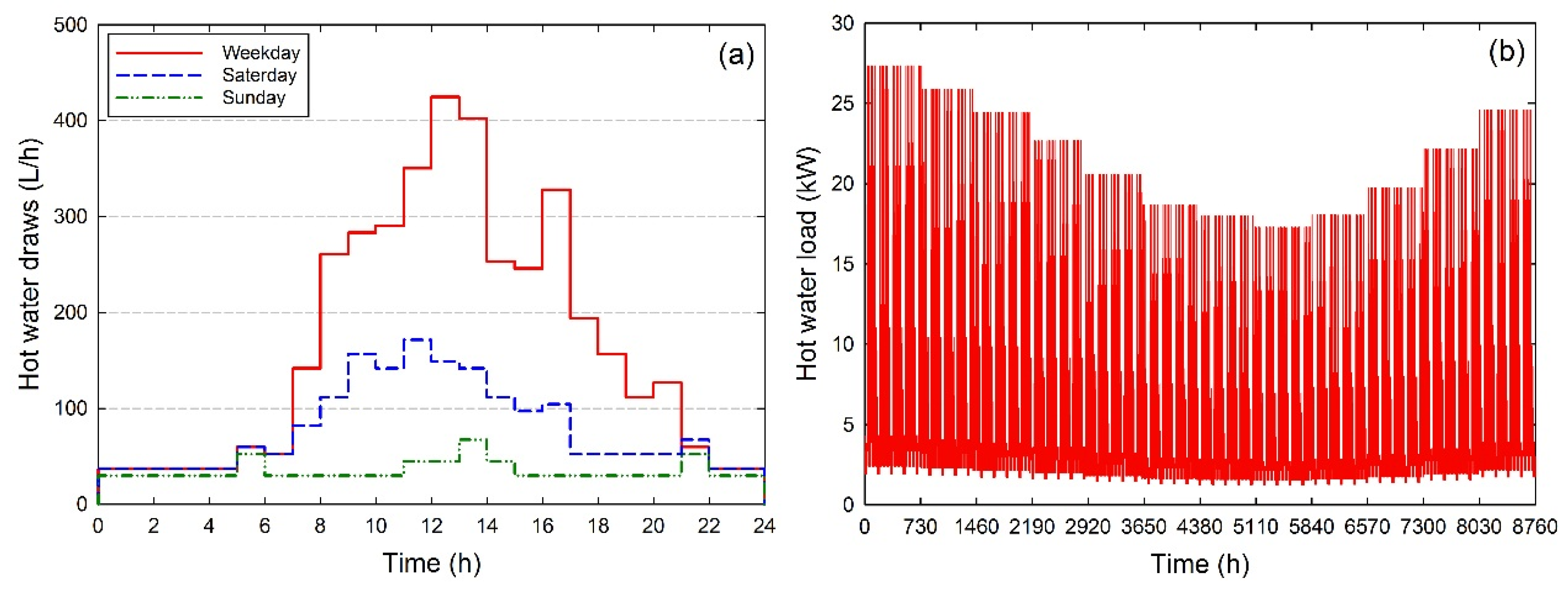
For the case studies, it was assumed that SWH system was installed in an office building. The distributions of hot water consumption for three different cases—a weekday, Saturday, and Sunday—based on the hot water load profile of a typical office building [23] are shown in Figure 3a. The hourly hot water load profile over one year is shown in Figure 3b. Weather data for Incheon (South Korea, latitude 36° N and longitude 125° E) were referred to. 
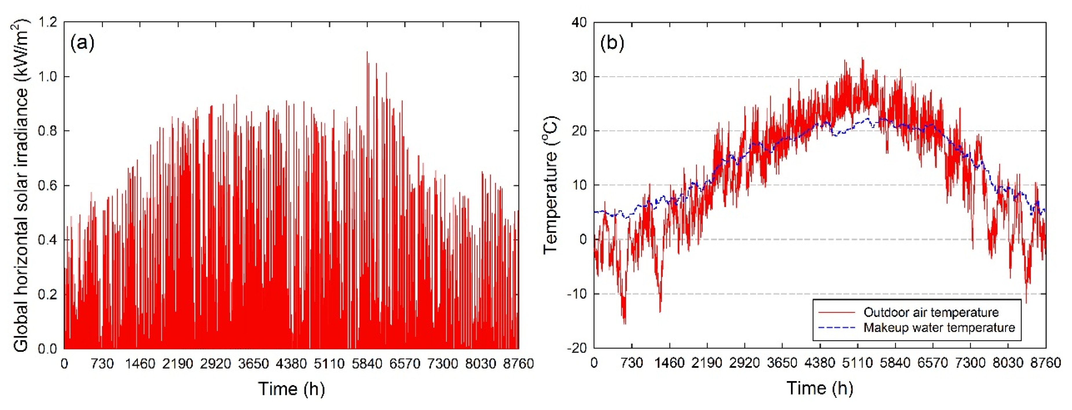
Figure 4 shows the hourly global horizontal solar irradiance, outdoor air temperature, and make-up water temperature.
Figure 3. (a) Hourly hot water consumption rates over one day; and (b) hot water load over one year in the building considered for the case studies.
Energies 08 11592 g003
Figure 4. (a) Hourly global horizontal solar irradiance; and (b) outdoor air temperature and make-up water temperature over one year for Incheon, South Korea.
Energies 08 11592 g004
The proposed method involved the use of various commercially available devices, and the set of devices used can be extended by the designer. The technical and economic characteristics of the solar collectors, heat exchangers, storage tanks, and auxiliary heaters used are summarized in the Table A1, Table A2, Table A3, Table A4 and Table A5 at the end of this paper. Table 1 shows the design parameters used as well as the assumptions made for the optimization process. Table 2 shows the electricity and LNG tariffs for an office building in South Korea.
Table 1. Optimization design parameters considered in case study.
ParameterDescriptionValue
γ Azimuth of collector array (Degrees)0
α s , w Meridian altitude in winter (° Degrees)29
T l Desired hot water temperature (°C)60
T s , m a x Maximum allowable storage tank temperature (°C)100
T a m b Temperature of environment surrounding storage tank (°C)20
c p , c Specific heat capacity of collector fluid (J/kg·°C)3843
c p , w Specific heat capacity of water (J/kg·°C)4153
ρ c o l l Density of collector fluid (kg/m3)1032
ρ w Density of water (kg/m3)991
η p Pumping efficiency of circulation pump (%)60
η m Motor efficiency of circulation pump (%)80
H p , h Head of pump on hot side of heat exchanger (m)80
H p , c Head of pump on cold side of heat exchanger (m)15
H p , l Head of pump on load side of SWH system (m)80
n p Project lifetime (years)40
i Real discount rate (%)2.91
e E L E Electricity cost escalation rate (%)4.00
e L N G Gas cost escalation rate (%)4.00
A R , m a x Maximum capacity available to receive subsidy cost (m2)500
A c o l l , m a x Area available to install solar collectors (m2)600
R I Supplementary cost ratio against purchase cost (%)30
R M Maintenance cost ratio against initial cost (%)1.5
R S Subsidy cost ratio against initial cost (%)50
Table 2. Electricity and LNG tariffs.
ClassificationValue
ElectricityBasic charge6160
Energy charge (KRW/kW·h)Summer (June, July, and August)105.7
Spring/Fall (March, April, May, September, and October)65.2
Winter (November, December, January, and February)92.3
Natural gasEnergy charge (KRW/MJ)Summer (May, June, July, August, and September)19.26
Spring/Fall (April, October, and November)19.28
Winter (December, January, February, and March)19.46

4.2. Optimization Results Based on Set of Design Variables

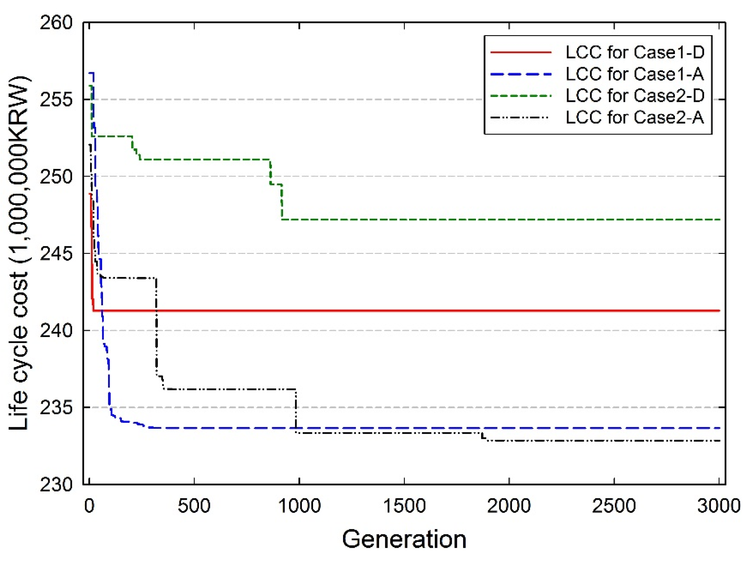
This case study aimed to optimize the design of SWH systems such that their LCC was minimized. Figure 5 shows the convergence of the objective functions of the four cases. The values of the objective function obtained for Case1-A and Case2-A are better than those obtained for Case1-D and Case2-D. In other words, the systems corresponding to Case1-A and Case2-A exhibited LCCs that were ~3.2% and ~6.1% lower than those for the systems corresponding to Case1-D and Case2-D, respectively. Figure 6 shows that the costs of the systems for Case1-A and Case2-A were lower than those of the systems for Case1-D and Case2-D; this was true for all cost items except the subsidy cost. Therefore, an optimization method that takes the installation and operation-related variables into account is obviously superior to one that only considers the capacity-related variables.
Table 3 shows a comparison of the results obtained for each case. As expected, the optimal values of the design variables and the corresponding values of the objective function varied for each case, depending on the set of the design variables.
Figure 5. Evolution of the objective functions for each case.
Energies 08 11592 g005
Figure 6. Comparison of the cost items for each case.
Energies 08 11592 g006
The capacity-related design variables for Case1-A and Case2-A, namely the volume of the storage tank and the heating capacity of the auxiliary heater, are the same as those for Case1-D and Case2-D, respectively. However, the area of the collector array and the overall heat transfer coefficient–area product of the heat exchanger for Case1-A and Case2-A were lower that those for Case1-D and Case2-D. The installation and operation-related design variables such as β c o l l , m c o l l , u , m h e x , c , Δ T o n , and Δ T o f f also vary. These differences in the design variables are analyzed in Figure 7 and Figure 8.
Table 3. Characteristics of the optimal SWH systems for each case.
ParameterClassification
Case1-DCase1-ACase2-DCase2-A
T c o l l (-)1444
N c o l l (ea.)3731121109
T h e x (-)961614
T t a n k (-)0066
T a u x (-)4444
N a u x (ea.)1111
β c o l l (°)35313539
m c o l l , u (kg/s·m2)0.01870.0110.01860.012
m h e x , c (kg/s)0.26110.26250.77280.9152
Δ T o n (°C)8787
Δ T o f f (°C)2121
A c o l l , t o t a l (m2)7461.38239.58215.82
U A h e x (W/°C)3489203593046978
V s (m3)0.960.966.216.21
q a u x , t o t a l (kW)34.8934.8934.8934.89
q L , p e a k (kW)27.3527.3527.3527.35
Q L , y e a r (kW·h/year)60218602186021860218
I T (kW·h/year)9716881004314591281083
Q u (kW·h/year)30664259896258955826
Q h e x (kW·h/year)24654247335115750626
Q l (kW·h/year)20721212781252
Q d (kW·h/year)9912587
Q L s (kW·h/year)24323243884798447914
Q a u x (kW·h/year)35895358301223412304
F S (%)40.3940.5079.6879.57
C L C C (1000 KRW)241278233668247854232854
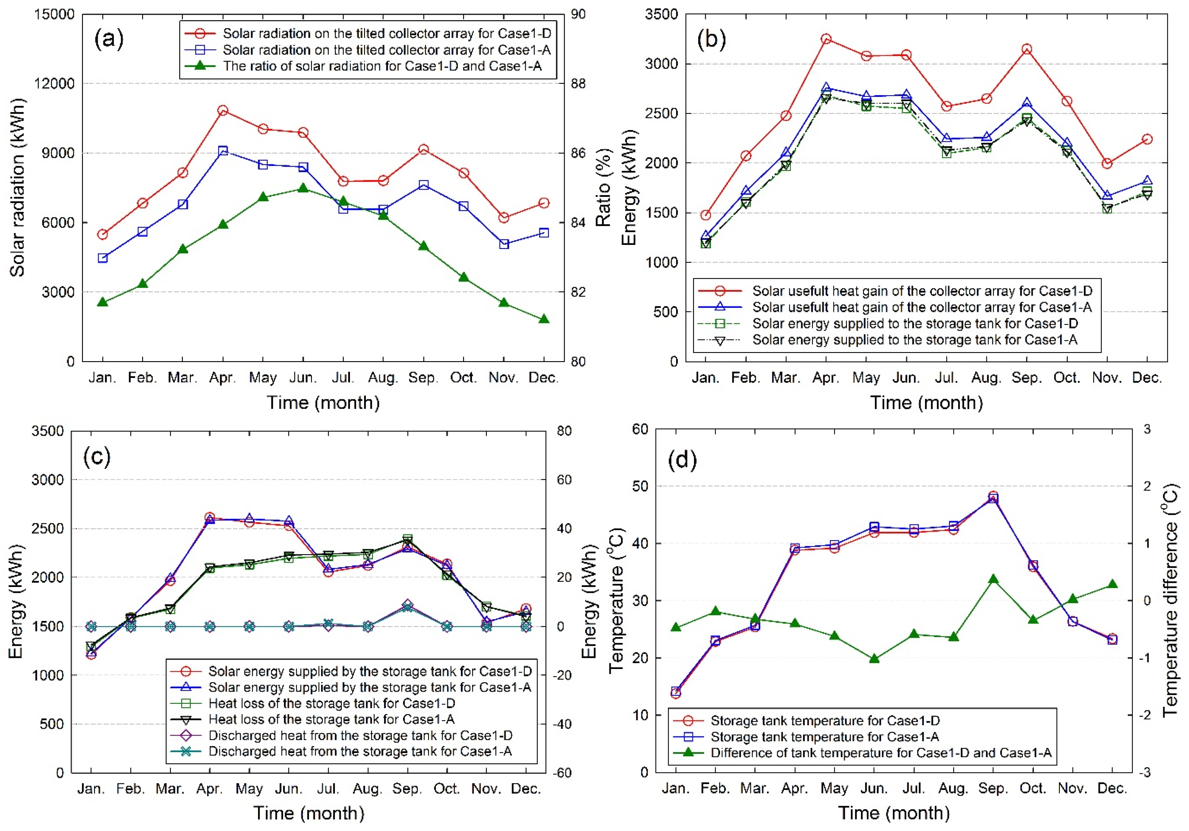
Figure 7 shows a comparison of the monthly energy performances of the optimal SWH systems corresponding to Case1-D and Case1-A. As shown in Figure 7a, the total solar radiation on the collector array of the optimal SWH system for Case1-A is ~16.6% lower than that for the optimal system for Case1-D. This is because of a 17.1% reduction in the area of the collector array. However, the slope of the collector array ( β c o l l ) is reduced from 35° to 31°, so that the decrease in the summer and the intermediate season is less than that in the winter. Depending on the decrease in the total solar radiation, as shown in Figure 7b, the useful solar heat gain for Case1-A is reduced by ~15.3%; however, the solar energy supplied to the storage tank is increased slightly by ~0.3%, compared to that for Case1-D. This results from an increase in the heat exchanger effectiveness which in turn, leads to an increase in the N T U and a decrease in the capacity rate ratio ( c r ), owing to a decrease in the mass flow rate on the hot side of the heat exchanger ( m c o l l , u ) and an increase in the mass flow rate on the cold side ( m h e x , c ). The value of ε for Case1-A is 0.932; this is ~16.7% higher compared to that (0.798) for Case1-D. In addition, it is assumed that the increase in the operating time of the circulation pump for Case1-A, owing to the decrease in Δ T o n and Δ T o f f , in contrast to Case1-D, allows for the supply of more solar energy to the storage tank. As shown in Figure 7c, the amounts of solar energy supplied by the storage tank ( Q L s ), the heat losses of the storage tank ( Q l ), and the amounts of heat discharged from the storage tank ( Q d ) on a monthly basis for Case1-A and Case1-D are very similar. Therefore, it can be seen from Figure 7d that the similarity between the monthly average storage tank temperatures for Case1-A and Case1-D are similar, even though the monthly average temperature for Case1-A is slightly higher than that for Case1-D for all months except September, November, and December. This is because of the decrease in β c o l l 
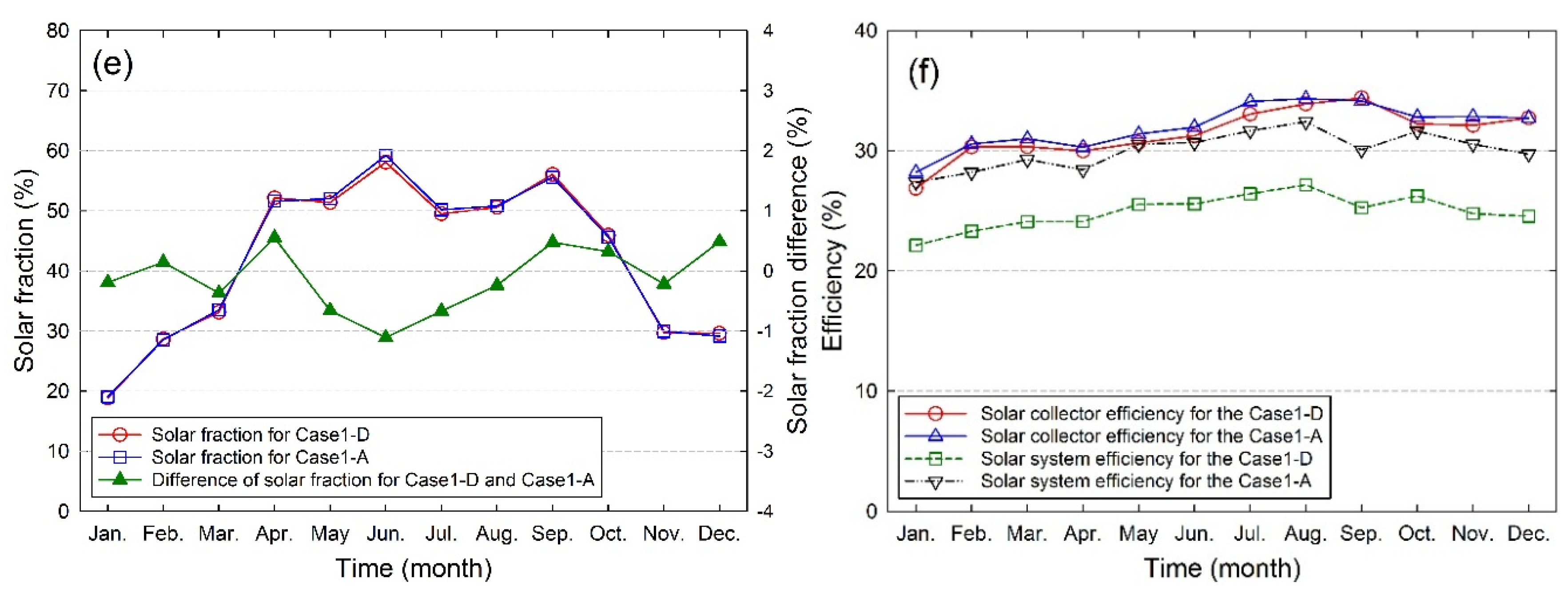
and the increase in the effectiveness of the heat exchanger. As a result, it can be seen from Figure 7e that the monthly solar fractions for Case1-A and Case1-D are very similar. However, owing to the effects of the installation and operation-related design variables (see Figure 7f), the annual collector efficiency and annual SWH system efficiency for Case1-A are ~1.2% and ~5.1%, respectively, higher than those of Case1-D. Therefore, the annual energy cost for Case1-A is ~0.9% lower than that for Case1-D.
Figure 7. Comparison of the monthly energy performances of optimal SWH systems corresponding to Case1-D and Case1-A: (a) solar radiation; (b) useful solar heat gain and solar energy supplied to the storage tank; (c) solar energy supplied by the storage tank, heat loss of the storage tank, and heat discharged from the storage tank; (d) storage tank temperature; (e) solar fraction; and (f) solar collector efficiency and solar system efficiency.
Energies 08 11592 g007aEnergies 08 11592 g007b
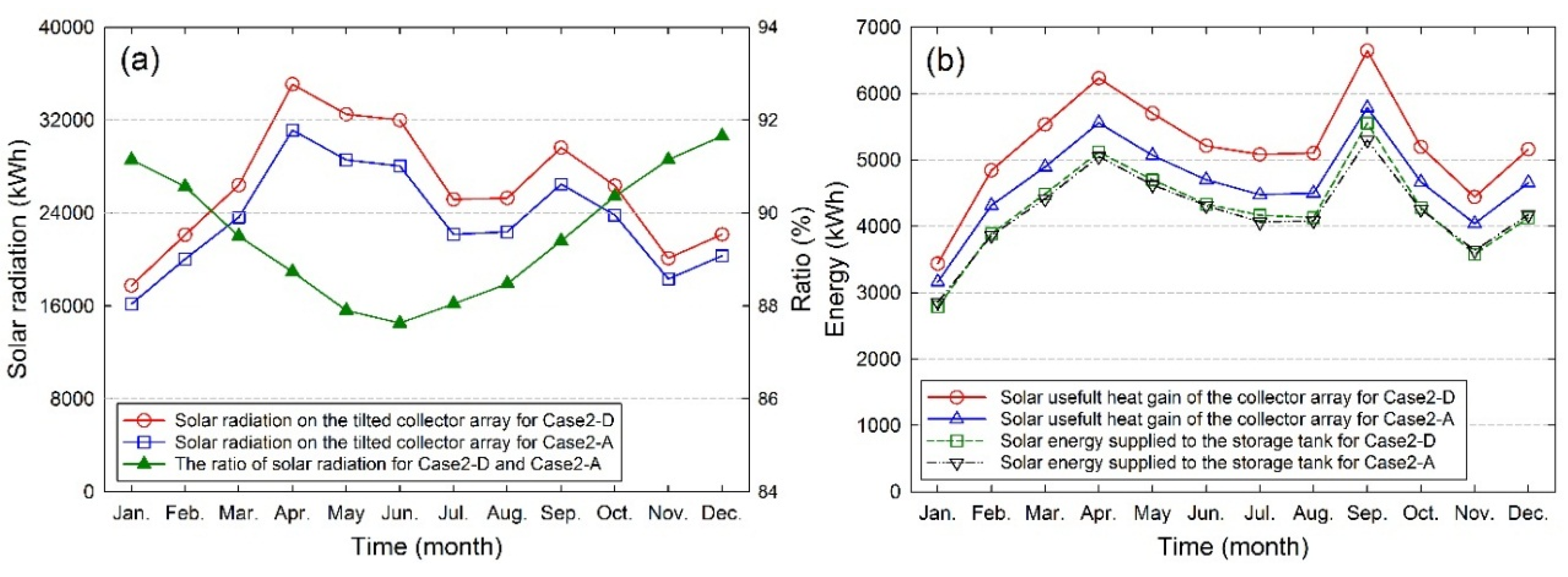
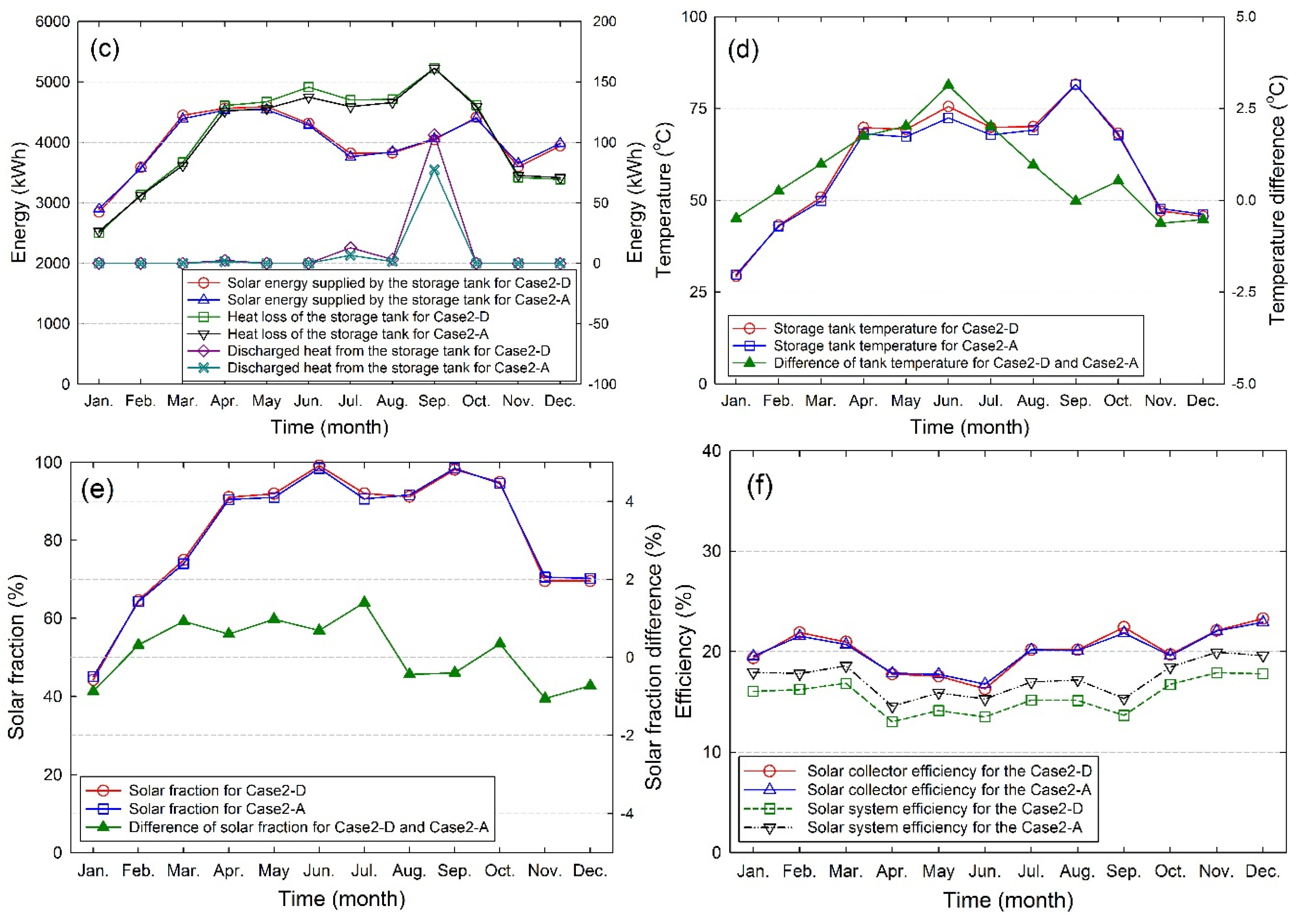
Figure 8 shows a comparison of the monthly energy performances of the optimal SWH systems corresponding to Case2-D and Case2-A and optimized at an annual solar fraction of 80%. Figure 8e shows that the monthly average solar fractions for Case2-D and Case2-A are 91.1%–99.2% and 90.5%–98.5%, respectively, from April to October. Therefore, it is more efficient to increase the solar fraction during winter because the solar fraction during the summer and the intermediate season is very close to the upper limit. Therefore, β c o l l for Case2-A is increased from 35° to 39° to collect more solar radiation in the winter. Figure 8 shows the changes in the annual energy performance caused by this increase. Furthermore, after decreasing m c o l l , u and increasing m h e x , c , the value of ε for Case2-A is 0.932, which is ~19.7% higher than that for Case2-D (0.779). Decreasing the Δ T o n and Δ T o f f values for Case2-A also increases the operating time of the circulation pump. Thanks to the optimization of the installation and the operation-related design variables, the decrease in the amount of solar energy supplied annually to the storage tank for Case2-A is only 1.0% compared to that for Case2-D. Furthermore, this decrease occurs primarily in the summer and the intermediate season; however, a greater amount of energy is supplied to the storage tank in the winter. Therefore, the annual SWH system efficiency for Case2-A is increased by ~2.25% and the annual energy cost is decreased by ~2.2% compared to those for Case2-D.
Figure 8. Comparison of the monthly energy performances of the optimal SWH systems corresponding to Case2-D and Case2-A: (a) solar radiation; (b) useful solar heat gain and solar energy supplied to the storage tank; (c) solar energy supplied by the storage tank, heat loss of the storage tank, and heat discharged from the storage tank; (d) storage tank temperature; (e) solar fraction; and (f) solar collector efficiency and solar system efficiency.
Energies 08 11592 g008aEnergies 08 11592 g008b

4.3. Parametric Study

Parametric studies were performed to evaluate the effects of five different installation and operation-related design variables— β c o l l , m c o l l , u , m h e x , c , Δ T o n , and Δ T o f f —on the energy and economic performances of the optimal SWH systems corresponding to Case1-A and Case2-A. The simulations were performed using the configurations and sizes of the optimal SWH systems corresponding to Case1-A and Case2-A.

4.3.1. Effect of Collector Slope

The effect of the collector slope on the energy and economic performances of the optimal SWH systems corresponding to Case1-A and Case2-A was simulated for β c o l l values ranging from 10° to 60°. Figure 9a shows that the annual solar fraction ( F S ) decreases and the energy cost and life cycle cost for 40 years increase when β c o l l is lower or higher than the optimal slope of 31°. The simulation results also indicate that β c o l l does not have a significant impact on the average annual collector array efficiency ( η c o l l ) and the average annual SWH system efficiency ( η s y s ). The energy and economic performances of the optimal SWH system corresponding to Case2-A also exhibit similar trends. Furthermore, Figure 9b shows that the energy cost and LCC for the optimal system corresponding to Case2-A increase mainly because of the high dependence on solar energy, that is, because F S is 80%. For example, as β c o l l decreases from 39° to 10°, the energy cost and LCC for 40 years increases by 22.0% and 6.54%, respectively. Meanwhile, the optimal collector slopes for Case1-A and Case2-A are in agreement with previously reported results [24,25,26].
Figure 9. Effect of collector slope on the LCC, annual solar fraction, and efficiency of the optimal SWH systems: (a) Case1-A and (b) Case2-A.
Energies 08 11592 g009

4.3.2. Effect of Mass Flow Rates of Collector

The effect of the collector’s mass flow rate on the energy and economic performances was simulated for m c o l l , u values ranging from 18 to 90 kg/h·m2. The mass flow rates on the cold side of the heat exchanger ( m h e x , c ) for systems corresponding to Case1-A and Case2-A were kept constant at 945.0 and 3294.7 kg/h, respectively. The variations in the energy and economic performances for Case1-A and Case2-A are plotted in Figure 10a and b, respectively. Figure 10a shows that F S and η s y s increase to their maximum values of ~40.5% and 30.1%, respectively, and the energy cost and LCC for 40 years decrease to their minimum values of ~178 and 233 million KRW, respectively, as m c o l l , u increases from 18 to 39.6 kg/h·m2. Next, F S and η s y s start to decrease, however, the costs and η c o l l increase, with a further increase in m c o l l , u . It was also observed that the maximum values of F S and η s y s correspond to and the minimum cost occurs at a m c o l l , u value of 39.6 kg/h·m2, which is the optimal value for Case1-A. As shown in Figure 10b, the simulation results for Case2-A are similar to those for Case1-A. However, for Case2-A, the variations in F S , η c o l l , and η s y s occur slowly whereas the variations in the energy and LCC occur rapidly compared to what was observed for Case1-A. The maximum values of F S and η s y s correspond to and the minimum cost occurs at a m c o l l , u value of 43.2 kg/h·m2, which is the optimal value for Case2-A. This is because the effectiveness of the heat exchanger ( ε ) decreases with the increase in m c o l l , u . The simulation results (not shown here) indicate that ε for Case1-A decreases from 0.932 to 0.662 as m c o l l , u increases from 39.6 to 90.0 kg/h·m2 and that ε for Case2-A decreases from 0.932 to 0.669 as m c o l l , u increases from 43.2 to 90.0 kg/h·m2. SWH systems with m c o l l , u values below the optimal values corresponding to Case1-A and Case2-A violate the constraint condition represented by Equation (44), because their flow rates are too low. Meanwhile, the optimum values of m c o l l , u in the primary circuit for Case1-A and Case2-A are in agreement with the results of a number of previous studies (50 kg/h·m2 [27], 18–48 kg/h·m2 [28], and 20–40 kg/h·m2 [29]).
Figure 10. Effect of mass flow rate per unit area of the collector on the energy and economic performance of the SWH systems: (a) Case1-A and (b) Case2-A.
Energies 08 11592 g010

4.3.3. Effect of Mass Flow Rates on Cold Side of Heat Exchanger

The variations in the energy and economic performances of the SWH systems were studied for mass flow rates on the cold side of the heat exchanger ( m h e x , c ) that were between 50% and 200% of those on the hot side of the heat exchanger, as indicated in Equation (43). Here, m c o l l , u for Case1-A and Case2-A were kept constant at 39.6 and 43.2 kg/h·m2, respectively. Figure 11 shows that F S , η c o l l , and η s y s decrease and the costs increase as m h e x , c decreases from the upper limit to the lower limit. Thus, the optimal values of m h e x , c for Case1-A and Case2-A are obtained at values close to the upper limit. The simulation results indicate that ε for Case1-A decreases from 0.932 to 0.812 as m h e x , c decreases from 945.0 to 450.0 kg/h and that ε for Case2-A decreases from 0.932 to 0.851 as m h e x , c decreases from 3294.7 to 1800.0 kg/h. SWH systems with m h e x , c values lower than 450.0 kg/h for Case1-A and 1800.0 kg/h for Case2-A violate the constraint condition represented by Equation (44), because the NTU value of the heat exchanger is greater than 4. This constraint has been set because increasing the NTU value beyond 3 or 4 usually results in an insignificant improvement in its effectiveness and thus, is not economically feasible. In addition, after the values that violated this constraint have been excluded, the simulation results indicate only a small improvement in the overall performance of the SWH system with the variation in m h e x , c in the secondary circuit. The optimum values of m h e x , c in the secondary circuit for Case1-A and Case2-A are 0.0043 and 0.0042 kg/s·m2, in terms of the mass flow rate-to-collector area ratio m h e x , c / ( A c o l l × N c o l l ) ). These values are in agreement with the typically reported values of 0.002–0.008 kg/s·m2 [13].
Figure 11. Effect of mass flow rate on the cold side of the heat exchanger on the energy and economic performances of the SWH systems: (a) Case1-A and (b) Case2-A.
Energies 08 11592 g011

4.3.4. Effect of Dead Band Temperature Difference

The effect of the difference in the temperatures of the upper and lower dead bands of the differential temperature controller on the energy and economic performances were studied. The values of the other design variables were kept constant at the optimum values. As shown in Figure 12, F S , η c o l l , and η s y s decrease slightly and the energy cost and LCC for 40 years increase as Δ T o n increases from 7 to 12 °C. Figure 13 shows a trend similar to that seen in Figure 12, with there being only a slight difference in the rate of change. The effect of Δ T o n on the overall performance of the SWH system is greater than that of Δ T o f f . Further, for high solar fractions, the rate of increase in the costs is greater than the rate of decrease in η c o l l and η s y s . These results show that there is only a small difference in the overall energy and economic performances of the SWH systems for different Δ T o n and Δ T o f f values.
Figure 12. Effect of a difference in the temperature of the upper dead band of the differential temperature controller on the energy and economic performances of the SWH systems: (a) Case1-A and (b) Case2-A.
Energies 08 11592 g012
Figure 13. Effect of a difference in the temperature of the lower dead band of the differential temperature controller on the energy and economic performances of the SWH systems: (a) Case1-A and (b) Case2-A.
Energies 08 11592 g013

5. Conclusions

In this paper, a novel design method is presented for optimizing the various design variables of an indirect forced circulation SWH system based on the LCC and using a GA. The effectiveness of the proposed method is assessed by analyzing the long-term performances of systems corresponding to four cases. The systems are optimized using different annual solar fractions and sets of design variables. The results show that the optimization method that takes into account the installation and operation-related design variables can reduce the LCC further by ~3.2% and ~6.1%, respectively, compared to the method that only considers the capacity-related design variables. Therefore, efficient and economical SWH systems can be designed by including the various design variables in the optimization process. In addition, parametric studies were performed to evaluate the effects of the installation and operation-related design variables on the energy and economic performances of the optimal SWH system determined using the proposed method. The results indicate that the slope and mass flow rate of the collector have a significant impact on the overall performance of the SWH system, whereas the mass flow rate in the secondary circuit and the difference in temperatures of the dead bands have a relatively small impact. Thus, it can be concluded that taking into account both the capacity and operation-related design variables, as is the case with the method proposed in this study, is helpful in maximizing the energy and economic performances of solar energy systems such as photovoltaic/thermal system, solar-driven absorption cooling systems, and solar-driven hybrid cooling, heating, and power systems.

Acknowledgments

This work was supported by the National Research Foundation of Korea (NRF) grant funded by the Korea government (MSIP) (NRF-2014R1A6A3A01059739).

Conflicts of Interest

The authors declare no conflict of interest.

Appendix

The technical and economic parameters of the solar collectors, heat exchangers, storage tanks, and auxiliary heaters are summarized in the following Tables. In addition, the Table A2 and Table A3 all show the specification of the heat exchangers used in the case studies.
Table A1. Technical and economic parameters of the solar collectors for each case.
ParametersTypes
01234
Intercept of collector efficiency (-)0.74450.72080.72000.71090.7043
Negative of slope of collector efficiency (W/m2·°C)4.84834.79994.09005.00504.5368
Flow rate of fluid under standard conditions (kg/s)0.03810.03730.04000.03680.0368
Overall height (m)2.002.002.002.022.00
Overall width (m)1.001.001.001.000.99
Lifetime (year)2020202020
Purchase cost (1000 KRW/ea.)545530520545540
Table A2. Technical and economic parameters of the heat exchangers for each case.
ParametersTypes
012345678
Overall heat transfer coefficient–area product (W/°C)465698930116314541745203523262908
Total heat transfer area (m2)0.17680.26520.30940.35360.44200.53040.61880.70720.8398
Area per plate (m2)0.04420.04420.04420.04420.04420.04420.04420.04420.0442
Total number of plates689101214161821
Lifetime (year)555555555
Purchase cost (1000 KRW/ea.)490520530540570590610640670
Table A3. Technical and economic parameters of the heat exchangers for each case.
ParametersTypes
910111213141516
Overall heat transfer coefficient–area product (W/°C)34894071465252345815697881419304
Total heat transfer area (m2)1.06081.23761.40001.54001.68002.10002.38002.8000
Area per a plate (m2)0.04420.04420.14000.14000.14000.14000.14000.1400
Total number of plates2630121314171922
Lifetime (year)55555555
Purchase cost (1000 KRW/ea.)730780105010701100117012201300
Table A4. Technical and economic parameters of the storage tanks for each case.
ParametersTypes
0123456
Tank volume (m3)0.961.722.653.764.915.546.21
Heat loss coefficient (W/°C)0.30.30.30.30.30.30.3
Overall height (m)1.221.522.002.442.442.442.44
Overall diameter (m)1.001.201.301.401.601.701.80
Lifetime (year)15151515151515
Purchase cost (1,000,000 KRW/ea.)7.159.4910.7312.6515.8817.3318.02
Table A5. Technical and economic parameters of the auxiliary heaters for each case.
ParametersTypes
012345
Rated heating capacity (kW)15.1218.6123.2629.0834.8958.15
Rated efficiency (%)838485868682
Lifetime (year)151515151515
Purchase cost (1000 KRW/ea.)80784490996410392291

References

  1. Hottel, H.C.; Whillier, A. Evaluation of Flat-Plate Collector Performance; University of Arizona Press: Tucson, AZ, USA, 1958. [Google Scholar]
  2. Klein, S.A. Calculation of flat-plate collector utilizability. Sol. Energy 1978, 21, 393–402. [Google Scholar] [CrossRef]
  3. Klein, S.A.; Beckman, W.A.; Duffie, J.A. A design procedure for solar heating systems. Sol. Energy 1976, 18, 113–127. [Google Scholar] [CrossRef]
  4. Klein, S.A.; Beckman, W.A. A general design method for closed-loop solar energy systems. Sol. Energy 1979, 22, 269–282. [Google Scholar] [CrossRef]
  5. Klein, S.A.; Cooper, P.I.; Freeman, T.L.; Beekman, D.L.; Beckman, W.A.; Duffie, J.A. A method of simulation of solar processes and its application. Sol. Energy 1975, 17, 29–37. [Google Scholar] [CrossRef]
  6. Lund, P.D.; Peltola, S.S. SOLCHIPS—A fast pre-design and optimization tool for solar heating with seasonal storage. Sol. Energy 1992, 48, 291–300. [Google Scholar] [CrossRef]
  7. Duffie, J.A.; Beckman, W.A. Solar Engineering of Thermal Processes, 3rd ed.; Wiley: Hoboken, NJ, USA, 2006. [Google Scholar]
  8. Yan, C.; Wang, S.; Ma, Z.; Shi, W. A simplified method for optimal design of solar water heating systems based on life-cycle energy analysis. Renew. Energy 2015, 74, 271–278. [Google Scholar] [CrossRef]
  9. Loomans, M.; Visser, H. Application of the genetic algorithm for optimization of large solar hot water systems. Sol. Energy 2002, 72, 427–439. [Google Scholar] [CrossRef]
  10. Krause, M.; Vajen, K.; Wiese, F.; Ackermann, H. Investigation on optimizing large solar thermal systems. Sol. Energy 2002, 73, 217–225. [Google Scholar] [CrossRef]
  11. Kalogirou, S.A. Optimization of solar systems using artificial neural-networks and genetic algorithms. Appl. Energy 2004, 77, 383–405. [Google Scholar] [CrossRef]
  12. Bornatico, R.; Pfeiffer, M.; Witzig, A.; Guzzella, L. Optimal sizing of a solar thermal building installation using particle swarm optimization. Energy 2012, 41, 31–37. [Google Scholar] [CrossRef]
  13. Kim, Y.D.; Thu, K.; Bhatia, H.K.; Bhatia, C.S.; Ng, K.C. Thermal analysis and performance optimization of a solar hot water plant with economic evaluation. Sol. Energy 2012, 86, 1378–1395. [Google Scholar] [CrossRef]
  14. Kulkarni, G.N.; Kedare, S.B.; Bandyopadhyay, S. Determination of design space and optimization of solar water heating systems. Sol. Energy 2007, 81, 958–968. [Google Scholar] [CrossRef]
  15. Atia, D.M.; Fahmy, F.H.; Ahmed, N.M.; Dorrah, H.T. Optimal sizing of a solar water heating system based on a genetic algorithm for an aquaculture system. Math. Comput. Model 2012, 55, 1436–1449. [Google Scholar] [CrossRef]
  16. Choi, D.S; Ko, M.J. Optimization design for a solar water heating system using the genetic algorithm. Int. J. Appl. Eng. Res. 2015, 10, 27031–27042. [Google Scholar]
  17. Herrando, M.; Markides, C.N.; Hellgardt, K. A UK-based assessment of hybrid PV and solar-thermal systems for domestic heating and power: System performance. Appl. Energy 2014, 122, 288–309. [Google Scholar] [CrossRef]
  18. Huang, B.J.; Lin, T.H.; Hung, W.C.; Sun, F.S. Performance evaluation of solar photovoltaic/thermal systems. Sol. Energy 2001, 5, 443–448. [Google Scholar] [CrossRef]
  19. Anderson, T.N.; Duke, M.; Morrison, G.L.; Carson, J.K. Performance of a building integrated photovoltaic/thermal (BIPVT) solar collector. Sol. Energy 2009, 83, 445–455. [Google Scholar] [CrossRef]
  20. Freeman, J.; Hellgardt, K.; Markides, C.N. An assessment of solar-powered organic Rankine cycle systems for combined heating and power in UK domestic applications. Appl. Energy 2015, 138, 605–620. [Google Scholar] [CrossRef]
  21. Henderson, H.; Huang, Y.J.; Parker, D. Residential Equipment Part Load Curve for Use in DOE-2: Technical Report LBNL-42175; Lawrence Berkeley National Laboratory: Berkeley, CA, USA, 1999. [Google Scholar]
  22. Kanpur Genetic Algorithms Laboratory. Available online: http://www.iitk.ac.in/kangal/codes.shtml (accessed on 29 January 2015).
  23. National Renewable Energy Laboratory. Available online: http://www.nrel.gov/docs/fy11osti/46861.pdf (accessed on 29 January 2015).
  24. Elminir, H.K.; Ghitas, A.E.; el-Hussainy, F.; Hamid, R.; Beheary, M.M.; Abdel-Moneim, K.M. Optimum solar flat-plate collector slope: Case study for Helwan, Egypt. Energy Convers. Manag. 2006, 47, 624–637. [Google Scholar] [CrossRef]
  25. Gunerhan, H.; Hepbasli, A. Determination of the optimum tilt angle of solar collectors for building applications. Build. Environ. 2007, 42, 779–783. [Google Scholar] [CrossRef]
  26. Qiu, G.; Riffat, S.B. Optimum tilt angle of solar collectors and its impact on performance. Int. J. Ambient Energy 2003, 24, 13–20. [Google Scholar] [CrossRef]
  27. Beckman, W.A.; Klein, S.A.; Duffie, J.A. Solar Heating Design by the F-chart Method; John Wiley: New York, NY, USA, 1977. [Google Scholar]
  28. Baughn, J.W.; Young, M.F. The calculated performance of a solar hot water system for a range of collector flow rates. Sol. Energy 1984, 32, 303–305. [Google Scholar] [CrossRef]
  29. Hobbi, A.; Siddiqui, K. Optimal design of a forced circulation solar water heating system for a residential unit in cold climate using TRNSYS. Sol. Energy 2009, 83, 700–714. [Google Scholar] [CrossRef]

