
Effects of Shear Dependent Viscosity and Variable Thermal Conductivity on the Flow and Heat Transfer in a Slurry

Abstract
:1. Introduction
2. Governing Equations of Motion and Heat Transfer
3. Constitutive Relations
3.1. Stress Tensor
3.2. Heat Flux Vector
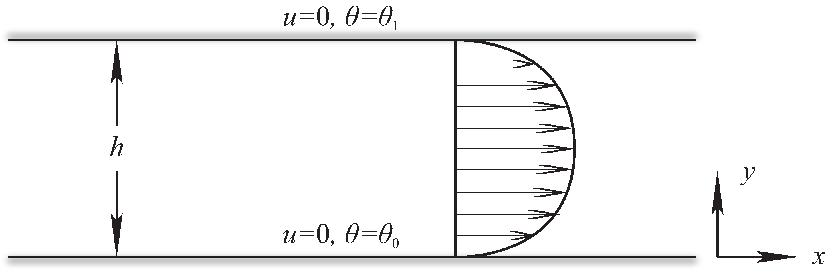
4. Geometry and the Kinematics of the Flow
5. Numerical Scheme

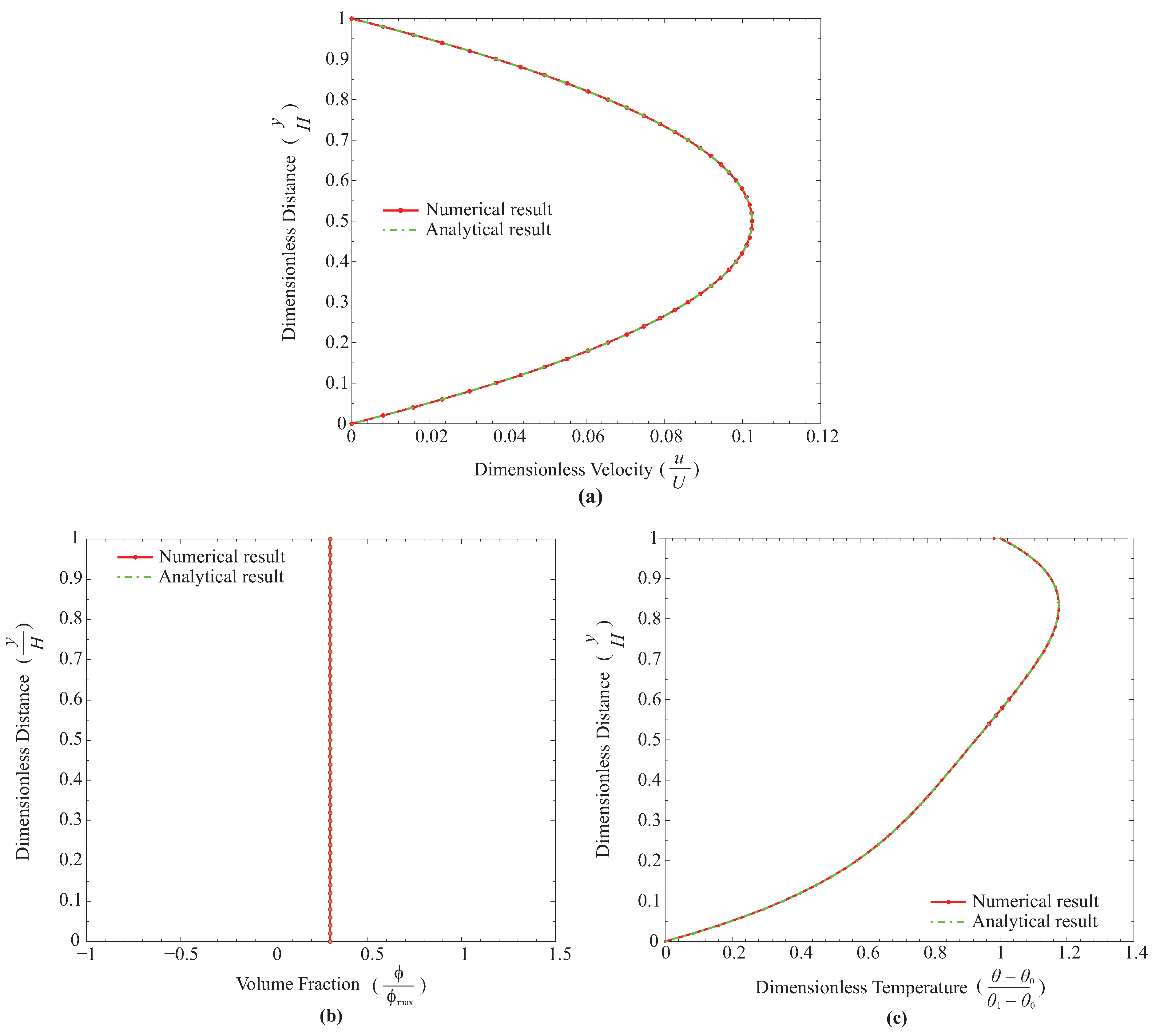
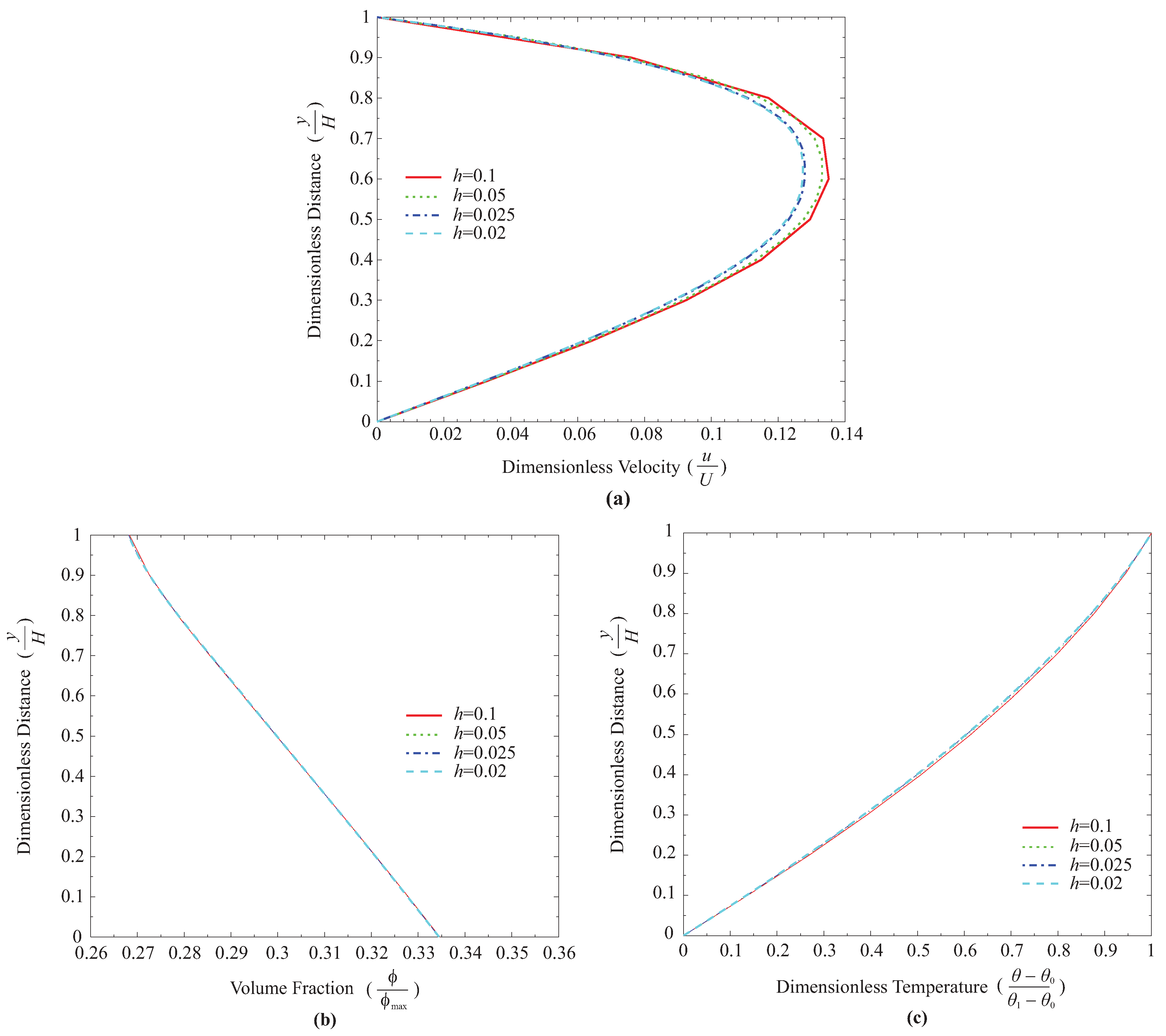
6. Results and Discussion

| m | M | B1 | B2 | B3 | B4 | R1 | R5 |
|---|---|---|---|---|---|---|---|
| −0.6, −0.3, 0, 0.3 | 0.1, 0.7, 1.2, 1.5 | −0.5, −1.5, −2, −3 | 0, 0.01, 0.02, 0.05 | 0, 10, 25, 50 | 0.05, 0.1, 0.2, 0.3 | 0, −0.1, −0.3, −0.8 | 0, 0.1, 2.5, 4 |
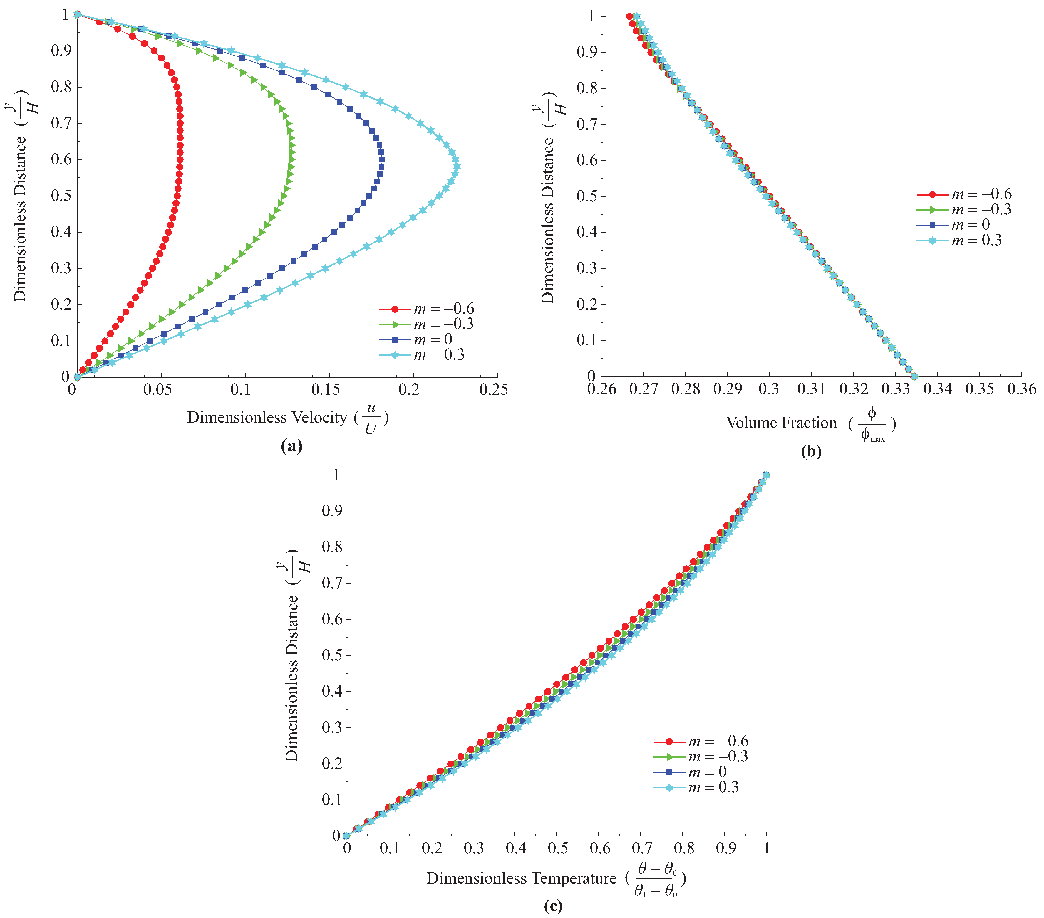
6.1. Effect of m

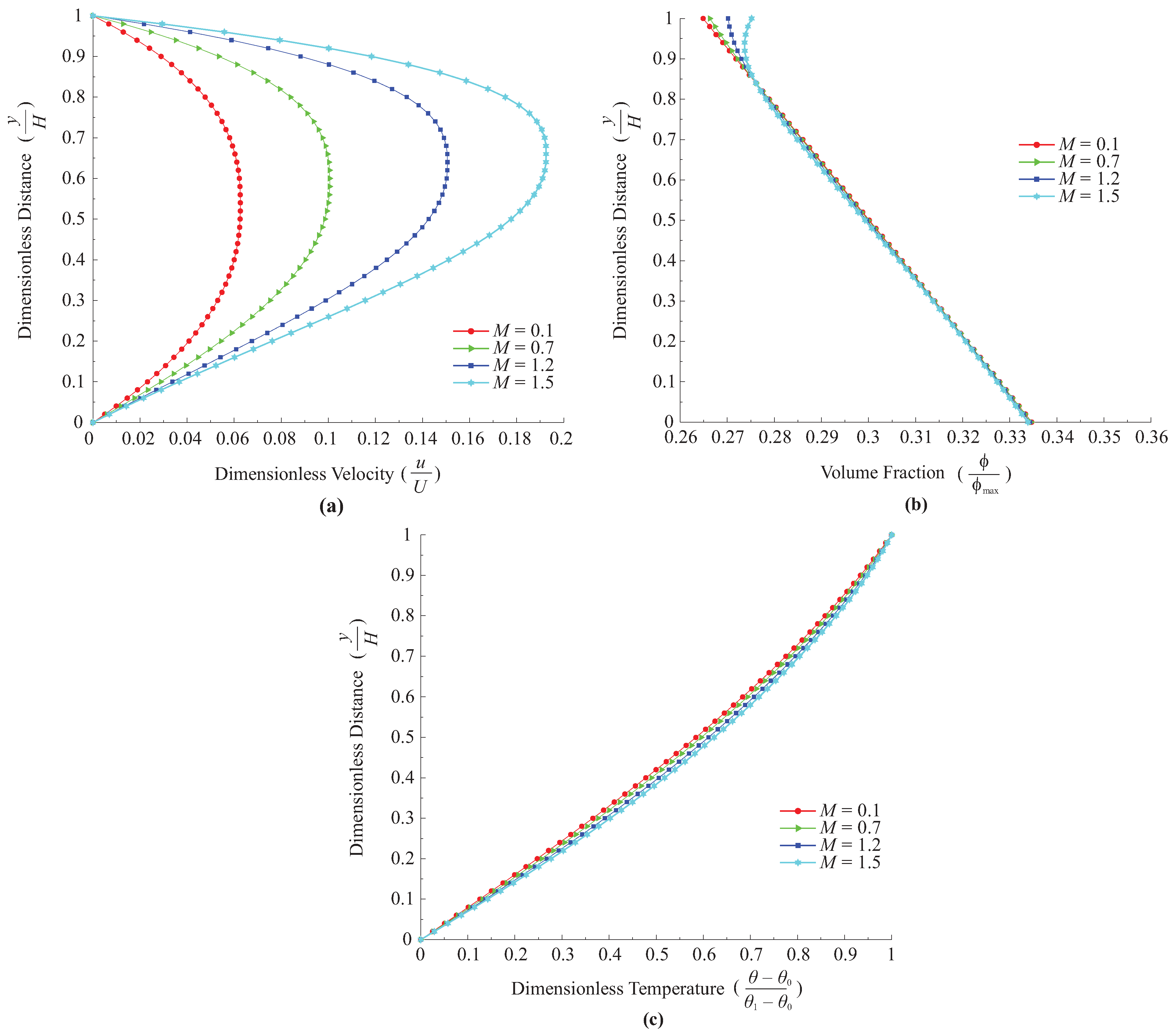
6.2. Effect of M
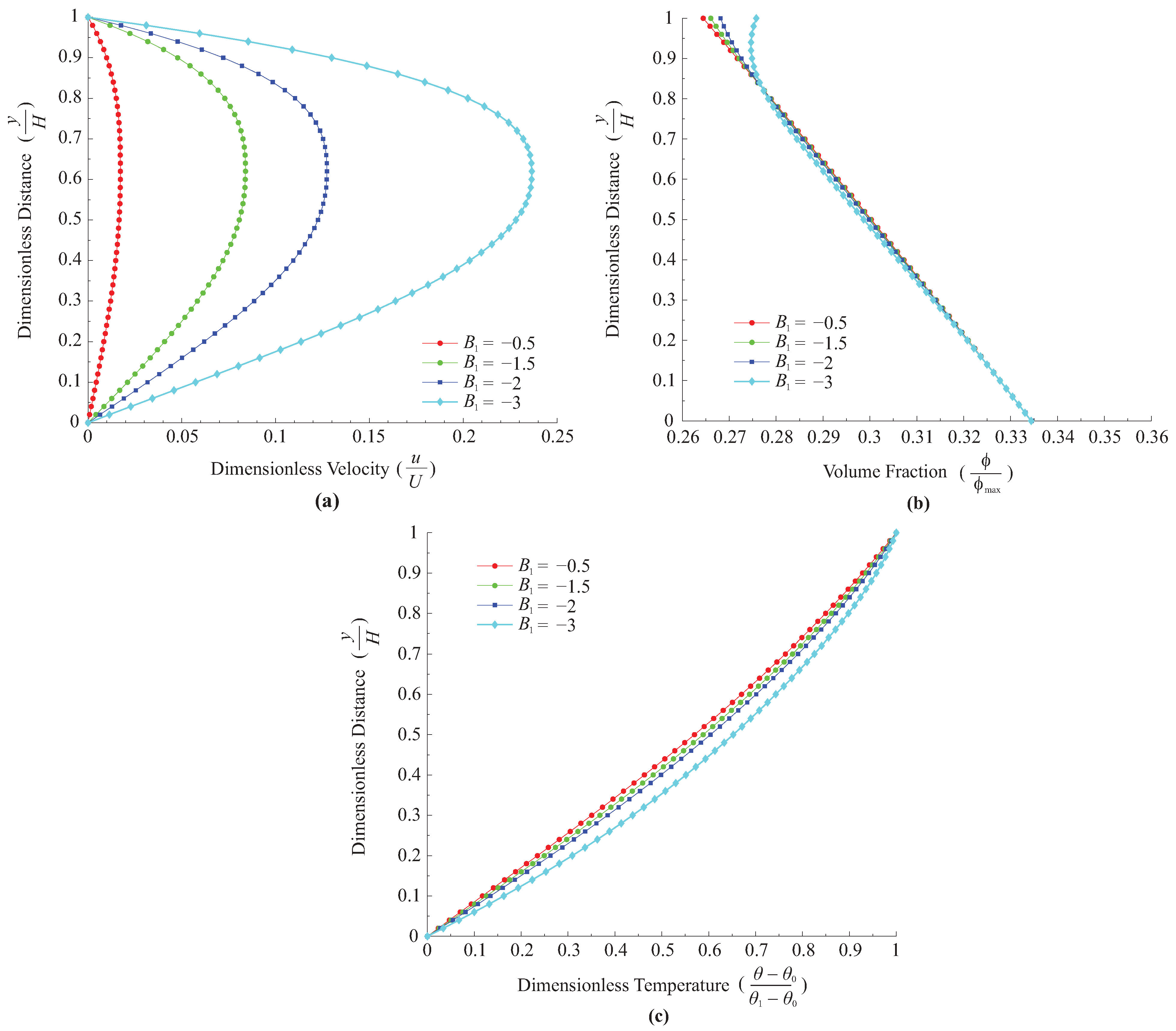
6.3. Effect of

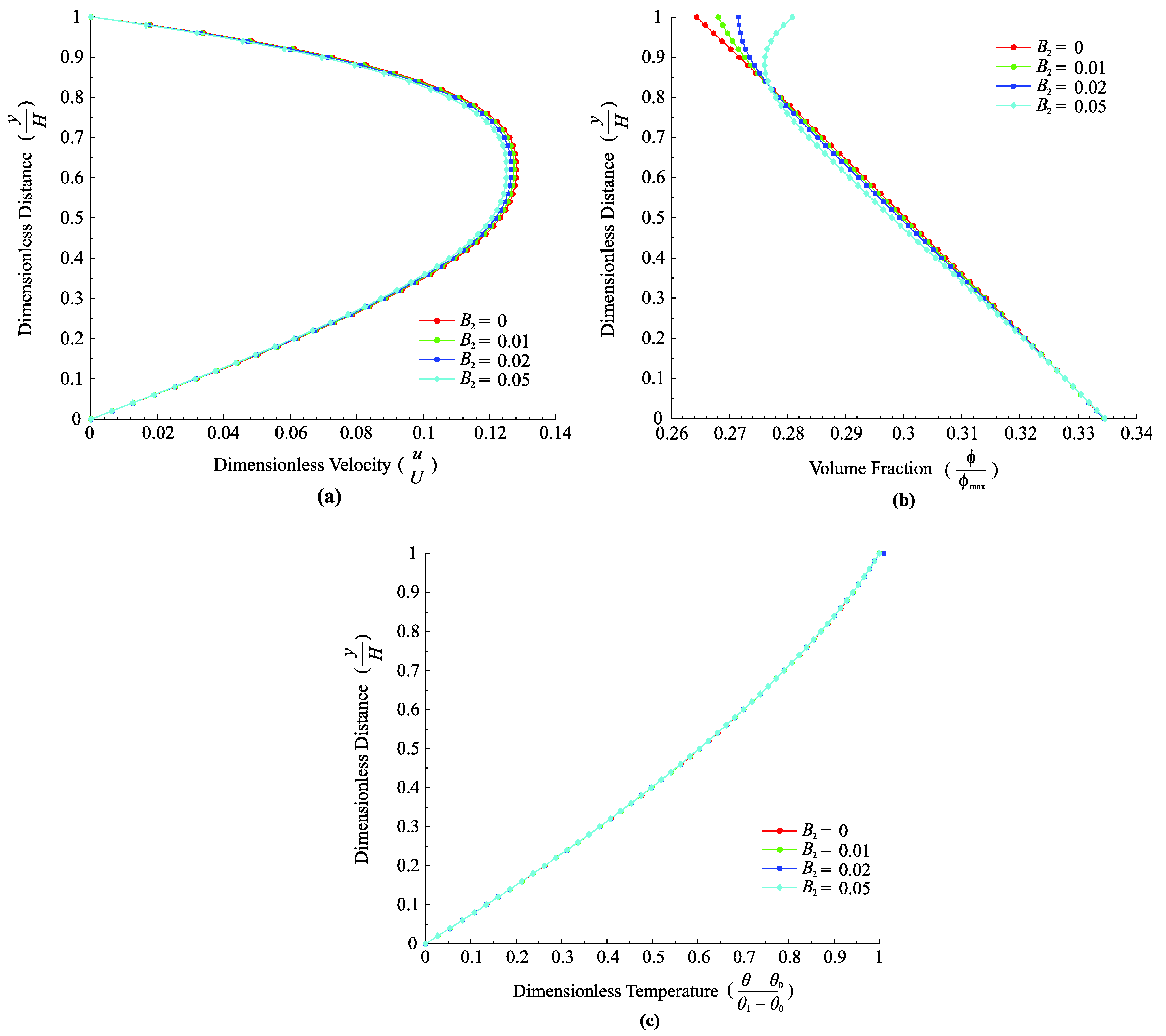
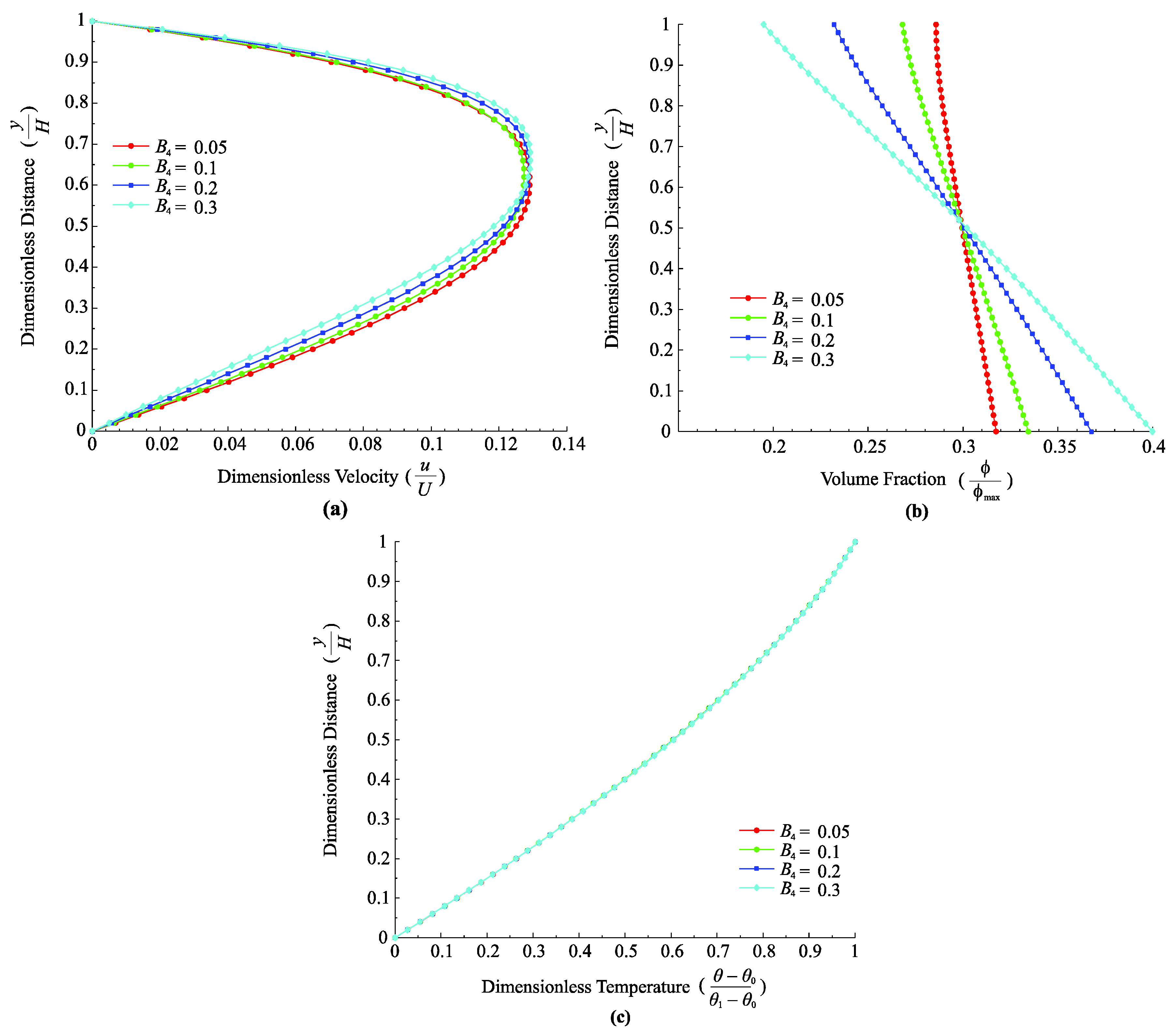
6.4. Effect of

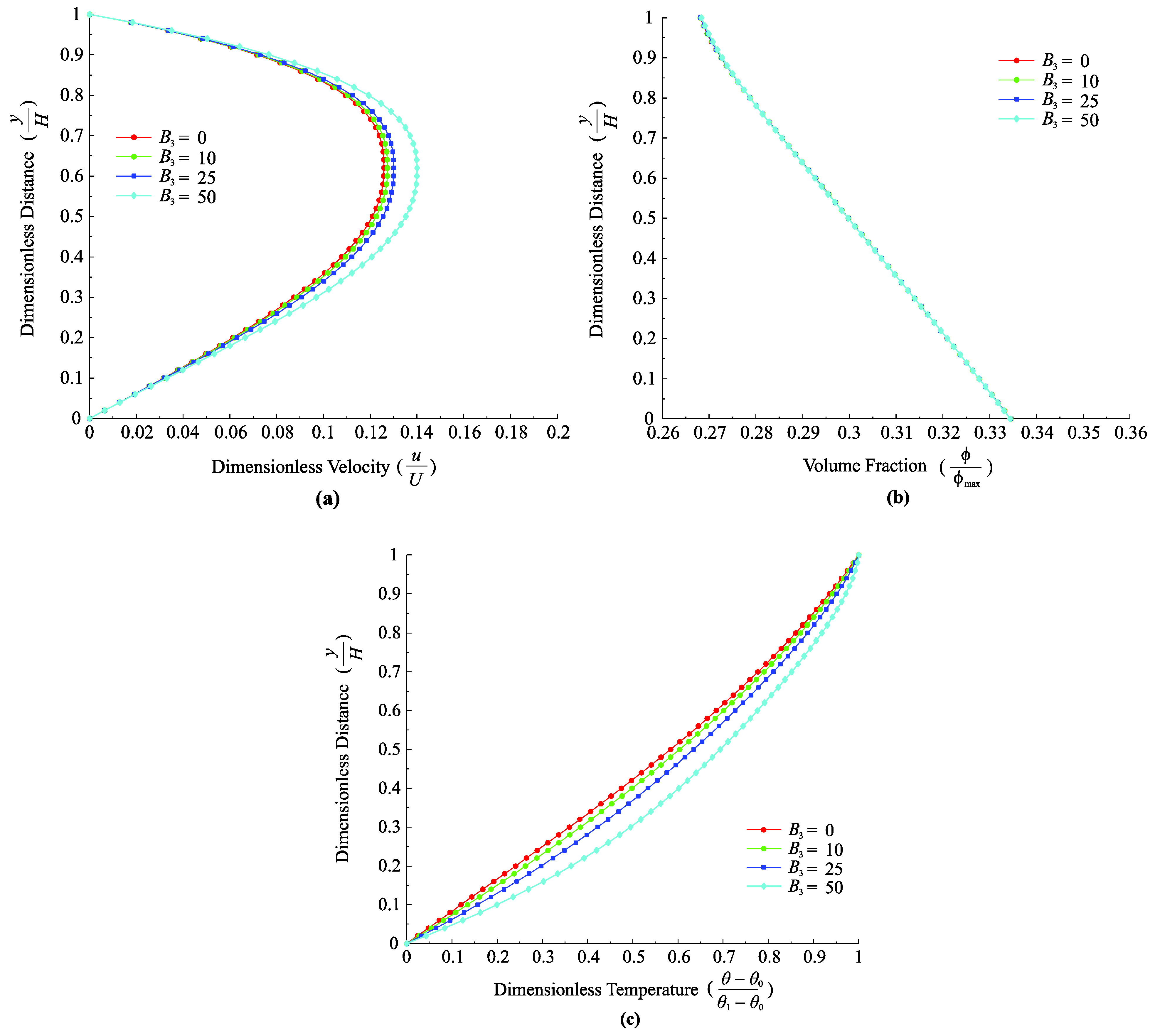
6.5. Effect of

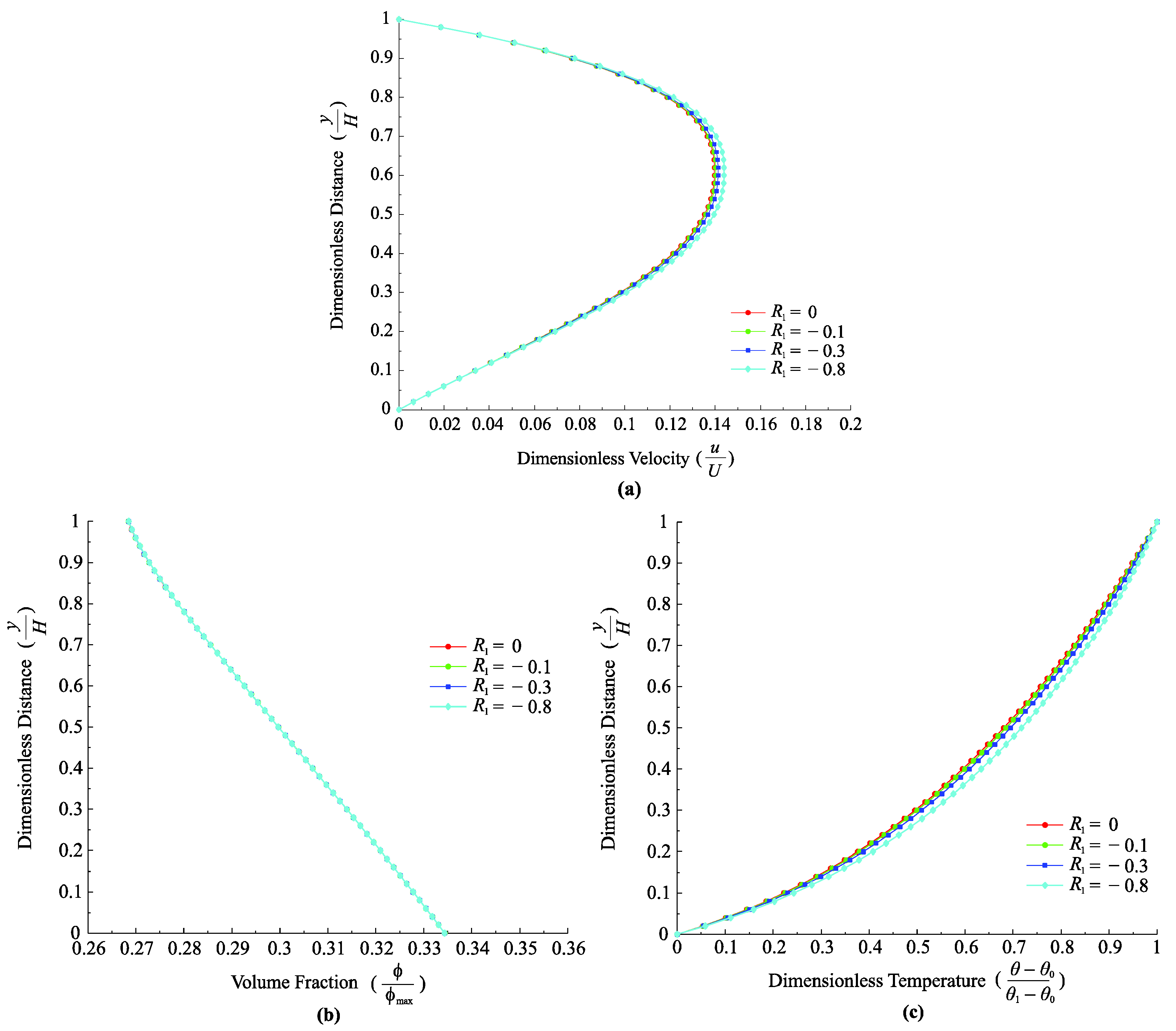
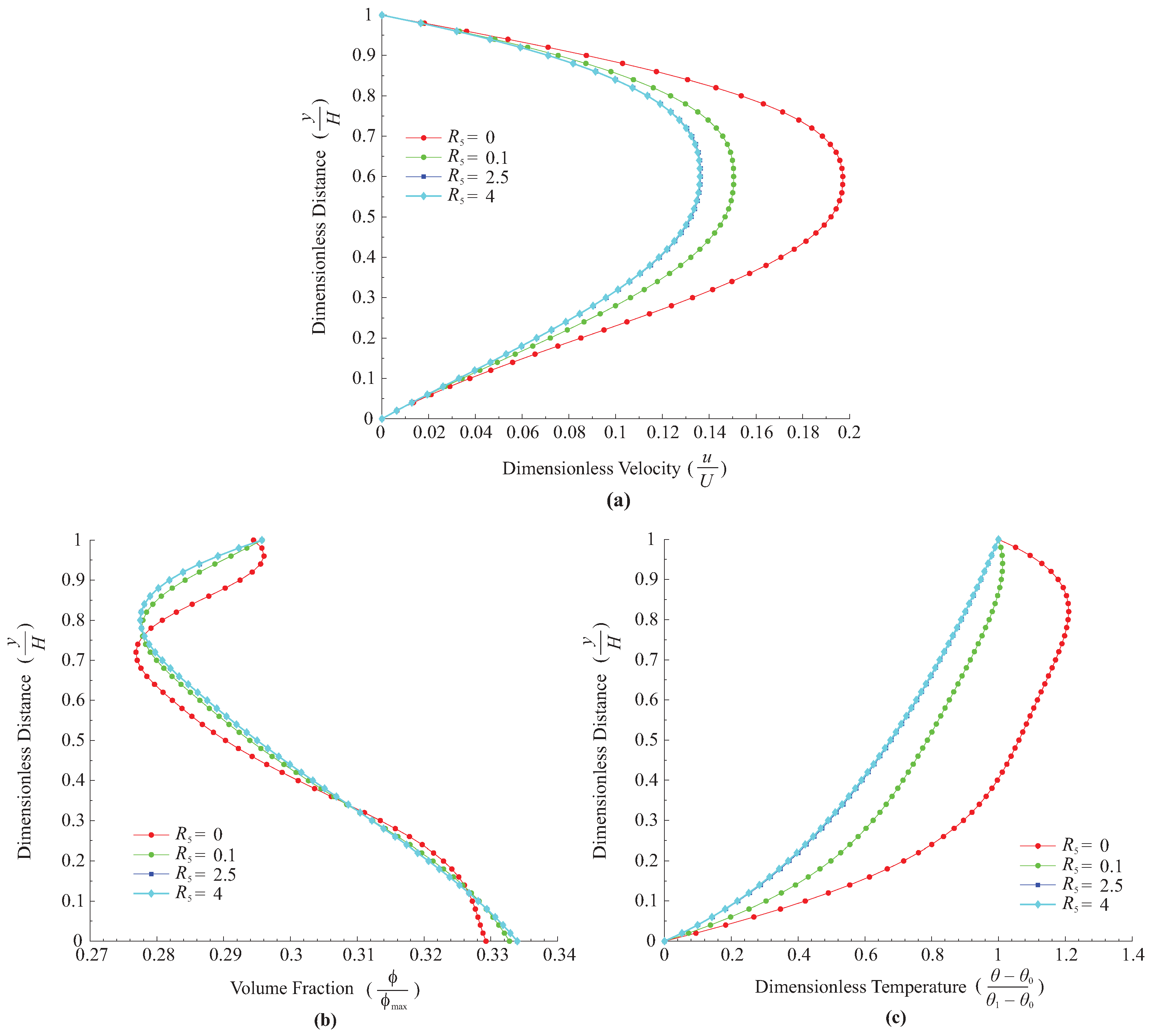
6.6. Effect of
6.7. Effect of and


6.8. Frictional Effects and Heat Transfer Rate at the Walls
| −0.6 | 0.1883 | −0.6369 | 4.1923 | −2.4930 | 1.2796 | 0.5923 |
| −0.3 | 0.3452 | −0.8454 | 3.8831 | −2.6550 | 1.3751 | 0.5319 |
| 0 | 0.4553 | −0.9291 | 3.7226 | −2.7744 | 1.4412 | 0.4950 |
| 0.3 | 0.5352 | −0.9696 | 3.6277 | −2.8686 | 1.4895 | 0.4691 |
| 0.1 | 0.2686 | −0.3164 | 3.2579 | −3.2819 | 1.2722 | 0.6258 |
| 0.7 | 0.3181 | −0.6068 | 3.6670 | −2.8412 | 1.3311 | 0.5724 |
| 1.2 | 0.3605 | −1.0436 | 4.0021 | −2.5193 | 1.4063 | 0.5020 |
| 1.5 | 0.3836 | −1.4328 | 4.1794 | −2.3314 | 1.4643 | 0.4468 |
| −0.5 | 0.0478 | −0.1172 | 0.9730 | −0.6656 | 1.1718 | 0.6931 |
| −1.5 | 0.2293 | −0.5622 | 2.9161 | −1.9954 | 1.2728 | 0.6025 |
| −2 | 0.3452 | −0.8454 | 3.8831 | −2.6550 | 1.3751 | 0.5319 |
| −3 | 0.6105 | −1.4852 | 5.7876 | −3.9417 | 1.7108 | 0.3427 |
| 0 | 0.3457 | −0.8395 | 3.8867 | −2.6419 | 1.1970 | 0.6189 |
| 10 | 0.3452 | −0.8454 | 3.8831 | −2.6550 | 1.3751 | 0.5319 |
| 25 | 0.3442 | −0.8537 | 3.8748 | −2.6732 | 1.6515 | 0.3957 |
| 50 | 0.3408 | −0.8632 | 3.8478 | −2.6940 | 2.1280 | 0.1589 |
7. Concluding Remarks
Author Contributions
Conflicts of Interest
References
- Lee, D.-L.; Irvine, T.F. Shear rate dependent thermal conductivity measurements of non-Newtonian fluids. Exp. Therm. Fluid Sci. 1997, 15, 16–24. [Google Scholar] [CrossRef]
- Massoudi, M. A note on the meaning of mixture viscosity using the classical continuum theories of mixtures. Int. J. Eng. Sci. 2008, 46, 677–689. [Google Scholar] [CrossRef]
- Ekmann, J.; Wildman, D.; Chen, J. Laminar flow studies of highly loaded suspensions in horizontal pipes. In Proceedings of the 2nd International Symposium on Slurry Flows, New York, NY, USA, June 1986; Volume 38, pp. 85–92.
- Massoudi, M. A Mixture Theory formulation for hydraulic or pneumatic transport of solid particles. Int. J. Eng. Sci. 2010, 48, 1440–1461. [Google Scholar] [CrossRef]
- Rajagopal, K.R.; Tao, L. Mechanics of Mixtures; World Scientific: River Edge, NJ, USA, 1995. [Google Scholar]
- Shenoy, A.; Mashelkar, R. Thermal convection in non-newtonian fluids. Adv. Heat Transf. 1982, 15, 59–141. [Google Scholar]
- Shenoy, A. Natural convection heat transfer to power-law fluids. In Handbook of Heat and Mass Transfer; Gulf Publishing: Houston, TX, USA, 1986. [Google Scholar]
- Keimanesh, M.; Rashidi, M.M.; Chamkha, A.J.; Jafari, R. Study of a third grade non-Newtonian fluid flow between two parallel plates using the multi-step differential transform method. Comput. Math. with Appl. 2011, 62, 2871–2891. [Google Scholar] [CrossRef]
- Ellahi, R. The effects of MHD and temperature dependent viscosity on the flow of non-Newtonian nanofluid in a pipe: Analytical solutions. Appl. Math. Model. 2013, 37, 1451–1467. [Google Scholar] [CrossRef]
- Bellet, D.; Sengelin, M.; Thirriot, C. Determination des proprietes thermophysiques de liquides non-Newtoniens a l’aide d'une cellule a cylindres coaxiaux. Int. J. Heat Mass Transf. 1975, 18, 1177–1187. [Google Scholar] [CrossRef]
- Lee, W.Y.; Cho, Y.I.; Hartnett, J.P. Thermal conductivity measurements of non-Newtonian fluids. Lett. Heat Mass Transf. 1981, 8, 255–259. [Google Scholar] [CrossRef]
- Cocci, A.A.; Picot, J.J.C. Rate of strain effect on the thermal conductivity of a polymer liquid. Polym. Eng. Sci. 1973, 13, 337–341. [Google Scholar] [CrossRef]
- Chitrangad, B.; Picot, J.J.C. Similarity in orientation effects on thermal conductivity and flow birefringence for polymers? Polydimethylsiloxane. Polym. Eng. Sci. 1981, 21, 782–786. [Google Scholar] [CrossRef]
- Wallace, D.J.; Moreland, C.; Picot, J.J.C. Shear dependence of thermal conductivity in polyethylene melts. Polym. Eng. Sci. 1985, 25, 70–74. [Google Scholar] [CrossRef]
- Loulou, T.; Peerhossaini, H.; Bardon, J.P. Etude experimentale de la conductivité thermique de fluides non-Newtoniens sous cisaillement application aux solutions de Carbopol 940. Int. J. Heat Mass Transf. 1992, 35, 2557–2562. [Google Scholar] [CrossRef]
- Chaliche, M.; Delaunay, D.; Bardon, J.P. Transfert de chaleur dans une configuration cône-plateau et mesure de la conductivité thermique en présence d’une vitesse de cisaillement. Int. J. Heat Mass Transf. 1994, 37, 2381–2389. [Google Scholar] [CrossRef]
- Shin, S. The effect of the shear rate-dependent thermal conductivity of non-newtonian fluids on the heat transfer in a pipe flow. Int. Commun. Heat Mass Transf. 1996, 23, 665–678. [Google Scholar] [CrossRef]
- Kostic, M.; Tong, H. Investigation of thermal conductivity of a polymer solution as function of shearing rate. ASME Proc. HTD 1999, 364, 15–22. [Google Scholar]
- Sohn, C.W.; Chen, M.M. Heat transfer enhancement in laminar slurry pipe flows with power law thermal conductivities. J. Heat Transfer 1984, 106, 539. [Google Scholar] [CrossRef]
- Charunyakorn, P.; Sengupta, S.; Roy, S.K. Forced convection heat transfer in microencapsulated phase change material slurries: flow in circular ducts. Int. J. Heat Mass Transf. 1991, 34, 819–833. [Google Scholar] [CrossRef]
- Lin, S.X.Q.; Chen, X.D.; Chen, Z.D.; Bandopadhayay, P. Shear rate dependent thermal conductivity measurement of two fruit juice concentrates. J. Food Eng. 2003, 57, 217–224. [Google Scholar] [CrossRef]
- Aguilera, J.; Stanley, D. Microstructural Principles of Food Processing and Engineering; Aspen Publishers Inc: Gaitherburg, MD, USA, 1999. [Google Scholar]
- Shin, S.; Lee, S.-H. Thermal conductivity of suspensions in shear flow fields. Int. J. Heat Mass Transf. 2000, 43, 4275–4284. [Google Scholar] [CrossRef]
- Lin, K.C.; Violi, A. Natural convection heat transfer of nanofluids in a vertical cavity: Effects of non-uniform particle diameter and temperature on thermal conductivity. Int. J. Heat Fluid Flow 2010, 31, 236–245. [Google Scholar] [CrossRef]
- Hojjat, M.; Etemad, S.G.; Bagheri, R.; Thibault, J. Thermal conductivity of non-Newtonian nanofluids: Experimental data and modeling using neural network. Int. J. Heat Mass Transf. 2011, 54, 1017–1023. [Google Scholar] [CrossRef]
- Yang, J.-C.; Li, F.-C.; Zhou, W.-W.; He, Y.-R.; Jiang, B.-C. Experimental investigation on the thermal conductivity and shear viscosity of viscoelastic-fluid-based nanofluids. Int. J. Heat Mass Transf. 2012, 55, 3160–3166. [Google Scholar] [CrossRef]
- Liu, I. Continuum Mechanics; Springer: Berlin, Germany, 2002. [Google Scholar]
- Müller, I. On the entropy inequality. Arch. Ration. Mech. Anal. 1967, 26, 118–141. [Google Scholar] [CrossRef]
- Ziegler, H. An Introduction to Thermomechanics, 2nd ed.; North-Holland Publishing Company: Amsterdam, The Netherlands, 1983. [Google Scholar]
- Truesdell, C.; Noll, W. The Non-Linear Field Theories of Mechanics; Springer: Berlin/Heidelberg, Germany, 1992. [Google Scholar]
- Gupta, G.; Massoudi, M. Flow of a generalized second grade fluid between heated plates. Acta Mech. 1993, 99, 21–33. [Google Scholar] [CrossRef]
- Tsai, S.C.; Knell, E.W. Viscometry and rheology of coal water slurry. Fuel 1986, 65, 566–571. [Google Scholar] [CrossRef]
- Saeki, T.; Usui, H. Heat transfer characteristics of coal-water mixtures. Can. J. Chem. Eng. 1995, 73, 400–404. [Google Scholar] [CrossRef]
- Schowalter, W.R. Mechanics of Non-Newtonian Fluids; Pergamon Press: Elmsford, NY, USA, 1977. [Google Scholar]
- Rivlin, R.; Ericksen, J. Stress-deformation relations for isotropic materials. J. Ration. Mech. Anal. 1955, 4, 323–425. [Google Scholar] [CrossRef]
- Massoudi, M.; Vaidya, A. On some generalizations of the second grade fluid model. Nonlinear Anal. Real World Appl. 2008, 9, 1169–1183. [Google Scholar] [CrossRef]
- Massoudi, M.; Wang, P. Slag behavior in gasifiers. Part II: constitutive modeling of slag. Energies 2013, 6, 807–838. [Google Scholar] [CrossRef]
- Miao, L.; Wu, W.-T.; Aubry, N.; Massoudi, M. Falling film flow of a viscoelastic fluid along a wall. Math. Methods Appl. Sci. 2014, 37, 2840–2853. [Google Scholar] [CrossRef]
- Miao, L.; Wu, W.-T.; Aubry, N.; Massoudi, M. Heat transfer and flow of a slag-type non-linear fluid: Effects of variable thermal conductivity. Appl. Math. Comput. 2014, 227, 77–91. [Google Scholar] [CrossRef]
- Man, C.-S. Nonsteady channel flow of ice as a modified second-order fluid with power-law viscosity. Arch. Ration. Mech. Anal. 1992, 119, 35–57. [Google Scholar] [CrossRef]
- Fosdick, R.; Rajagopal, K. Anomalous features in the model of “second order fluids”. Arch. Ration. Mech. Anal. 1979, 70, 145–152. [Google Scholar] [CrossRef]
- Dunn, J.E.; Rajagopal, K.R. Fluids of differential type: Critical review and thermodynamic analysis. Int. J. Eng. Sci. 1995, 33, 689–729. [Google Scholar] [CrossRef]
- Reynolds, O. On the theory of lubrication and its application to Mr. Beauchamp Tower’s experiments, including an experimental determination of the viscosity of olive oil. Philos. Trans. R. Soc. London 1886, 177, 157–234. [Google Scholar] [CrossRef]
- Roscoe, R. The viscosity of suspensions of rigid spheres. Br. J. Appl. Phys. 1952, 3, 267–269. [Google Scholar] [CrossRef]
- Roscoe, R. Suspensions. In Flow Properties of Disperse Systems; North-Holland Pub. Co.: Amsterdam, The Netherlands, 1953; pp. 1–38. [Google Scholar]
- Dunn, J.E.; Fosdick, R.L. Thermodynamics, stability, and boundedness of fluids of complexity 2 and fluids of second grade. Arch. Ration. Mech. Anal. 1974, 56, 191–252. [Google Scholar] [CrossRef]
- Fourier, J.-B.-J. The Analytical Theory of Heat; Cambridge the University Press: London, UK, 1878. [Google Scholar]
- Fourier, J.-B.-J. The Analytical Theory of Heat; Dover Publishers: New York, NY, USA, 1955. [Google Scholar]
- Truesdell, C. Thermodynamics of Diffusion. In Rational Thermodynamics; Springer: New York, NY, USA, 1984; pp. 219–236. [Google Scholar]
- Winterton, R.H.S. Early study of heat transfer: Newton and Fourier. Heat Transf. Eng. 2001, 22, 3–11. [Google Scholar] [CrossRef]
- Liu, I.-S. On Fourier’s law of heat conduction. Contin. Mech. Thermodyn. 1990, 2, 301–305. [Google Scholar] [CrossRef]
- Bashir, Y.M.; Goddard, J.D. Experiments on the conductivity of suspensions of ionically-conductive spheres. AIChE J. 1990, 36, 387–396. [Google Scholar] [CrossRef]
- Prasher, R.S.; Koning, P.; Shipley, J.; Devpura, A. Dependence of thermal conductivity and mechanical rigidity of particle-laden polymeric thermal interface material on particle volume fraction. J. Electron. Packag. 2003, 125, 386. [Google Scholar] [CrossRef]
- Kaviany, M. Principles of Heat Transfer in Porous Media; Springer-Verlag: New York, NY, USA, 1995. [Google Scholar]
- Ingham, D.B.; Pop, I.I. Transport phenomena in porous media; Pergamon: Oxford, UK, 1998. [Google Scholar]
- Batchelor, G.K. Transport properties of two-phase materials with random structure. Annu. Rev. Fluid Mech. 1974, 6, 227–255. [Google Scholar] [CrossRef]
- Massoudi, M. On the heat flux vector for flowing granular materials—Part I: effective thermal conductivity and background. Math. Methods Appl. Sci. 2006, 29, 1585–1598. [Google Scholar] [CrossRef]
- Massoudi, M. On the heat flux vector for flowing granular materials—part II: derivation and special cases. Math. Methods Appl. Sci. 2006, 29, 1599–1613. [Google Scholar] [CrossRef]
- Bowen, R.M. Introduction to Continuum Mechanics for Engineers; Plenum Press: New York, NY, USA, 1989. [Google Scholar]
- Soto, R.; Mareschal, M.; Risso, D. Departure from fourier’s law for fluidized granular media. Phys. Rev. Lett. 1999, 83, 5003–5006. [Google Scholar] [CrossRef]
- Wang, L. Vector-field theory of heat flux in convective heat transfer. Nonlinear Anal. Theory Methods Appl. 2001, 47, 5009–5020. [Google Scholar] [CrossRef]
- Yang, H.; Aubry, N.; Massoudi, M. Heat transfer in granular materials: Effects of nonlinear heat conduction and viscous dissipation. Math. Methods Appl. Sci. 2013, 36, 1947–1964. [Google Scholar] [CrossRef]
- Rodrigues, J.; Urbano, J. On the stationary Boussinesq-Stefan problem with constitutive power-laws. Int. J. Non. Linear. Mech. 1998, 33, 555–566. [Google Scholar] [CrossRef]
- Massoudi, M.; Christie, I. Effects of variable viscosity and viscous dissipation on the flow of a third grade fluid in a pipe. Int. J. Non. Linear. Mech. 1995, 30, 687–699. [Google Scholar] [CrossRef]
- Chhabra, R.; Richardson, J. Non-Newtonian Flow and Applied Rheology; Butterworth-Heinemann: Oxford, UK, 2008. [Google Scholar]
- Phan-Thien, N.; Fang, Z.; Graham, A.L. Stability of some shear flows for concentrated suspensions. Rheol. Acta 1996, 35, 69–75. [Google Scholar] [CrossRef]
- Kusaka, Y.; Fukasawa, T.; Adachi, Y. Cluster-cluster aggregation simulation in a concentrated suspension. J. Colloid Interface Sci. 2011, 363, 34–41. [Google Scholar] [CrossRef] [PubMed]
- Johnson, G.; Massoudi, M.; Rajagopal, K.R. Flow of a fluid infused with solid particles through a pipe. Int. J. Eng. Sci. 1991, 29, 649–661. [Google Scholar] [CrossRef]
- Johnson, G.; Massoudi, M.; Rajagopal, K.R. Flow of a fluid—solid mixture between flat plates. Chem. Eng. Sci. 1991, 46, 1713–1723. [Google Scholar] [CrossRef]
- Ho, B.P.; Leal, L.G. Migration of rigid spheres in a two-dimensional unidirectional shear flow of a second-order fluid. J. Fluid Mech. 2006, 76, 783. [Google Scholar] [CrossRef]
- Pasquino, R.; Snijkers, F.; Grizzuti, N.; Vermant, J. The effect of particle size and migration on the formation of flow-induced structures in viscoelastic suspensions. Rheol. Acta 2010, 49, 993–1001. [Google Scholar] [CrossRef]
- Leal, L.G. Particle motions in a viscous fluid. Annu. Rev. Fluid Mech. 1980, 12, 435–476. [Google Scholar] [CrossRef]
- Schonberg, J.A.; Hinch, E.J. Inertial migration of a sphere in poiseuille flow. J. Fluid Mech. 1989, 203, 517–524. [Google Scholar] [CrossRef]
- Lecampion, B.; Garagash, D.I. Confined flow of suspensions modelled by a frictional rheology. J. Fluid Mech. 2014, 759, 197–235. [Google Scholar] [CrossRef]
- Boyer, F.; Guazzelli, É.; Pouliquen, O. Unifying suspension and granular rheology. Phys. Rev. Lett. 2011, 107, 188301. [Google Scholar] [CrossRef] [PubMed]
© 2015 by the authors; licensee MDPI, Basel, Switzerland. This article is an open access article distributed under the terms and conditions of the Creative Commons Attribution license (http://creativecommons.org/licenses/by/4.0/).
Share and Cite
Miao, L.; Massoudi, M. Effects of Shear Dependent Viscosity and Variable Thermal Conductivity on the Flow and Heat Transfer in a Slurry. Energies 2015, 8, 11546-11574. https://doi.org/10.3390/en81011546
Miao L, Massoudi M. Effects of Shear Dependent Viscosity and Variable Thermal Conductivity on the Flow and Heat Transfer in a Slurry. Energies. 2015; 8(10):11546-11574. https://doi.org/10.3390/en81011546
Chicago/Turabian StyleMiao, Ling, and Mehrdad Massoudi. 2015. "Effects of Shear Dependent Viscosity and Variable Thermal Conductivity on the Flow and Heat Transfer in a Slurry" Energies 8, no. 10: 11546-11574. https://doi.org/10.3390/en81011546