Designing a Profit-Maximizing Critical Peak Pricing Scheme Considering the Payback Phenomenon

Abstract

Critical peak pricing (CPP) is a demand response program that can be used to maximize profits for a load serving entity in a deregulated market environment. Like other such programs, however, CPP is not free from the payback phenomenon: a rise in consumption after a critical event. This payback has a negative effect on profits and thus must be appropriately considered when designing a CPP scheme. However, few studies have examined CPP scheme design considering payback. This study thus characterizes payback using three parameters (duration, amount, and pattern) and examines payback effects on the optimal schedule of critical events and on the optimal peak rate for two specific payback patterns. This analysis is verified through numerical simulations. The results demonstrate the need to properly consider payback parameters when designing a profit-maximizing CPP scheme.

1. Introduction

Demand response (DR) programs give customers a more active role in the operation of the power system, allowing them to change their consumption patterns. They have been implemented to ensure secure power system operation when the system suffers from severe supply-demand imbalances [1]. The main operators of DR programs are load serving entities (LSEs) that supply electricity to contracted customers (i.e., utilities). Recent deregulation of the power industry has made it possible for DR programs to be implemented in a market environment [2]. Accordingly, an LSE could become a demand-side participant in the market, aiming to maximize its profit through the DR program [3].

In a market context, the LSE’s profit depends on the difference between the purchase and resale prices. The purchase prices are determined for a specified time interval (e.g., every five min) based on the supply and demand for electricity [4]. They are inherently time-varying, and will be denoted here as “real-time market clearing prices” (RTMCPs). Since the resale (or retail) rates are relatively fixed compared to the RTMCPs, a sudden increase in the RTMCP leads to a corresponding reduction in the LSE’s profits [5]. As a result, dynamic pricing schemes are typically designed and included in DR programs to take variations in the RTMCPs into consideration [6].

Such dynamic pricing schemes include three main approaches: real-time pricing (RTP), time-of-use (TOU), and peak pricing (CPP) [6]. This study focuses on CPP, which has certain advantages over RTP and TOU. In RTP, customers are exposed to continuously changing prices; they must thus repeatedly decide whether to respond to price changes in order to reduce their electricity bills. By contrast, in a CPP scheme, customers must make decisions about whether to reduce consumption only when critical events occur. Thus, CPP is simpler to implement than RTP, particularly for residential customers [7]. TOU is also easy to implement, as it consists only of a few block rates. However, these rates must be announced to customers in advance, making TOU unable to manage sudden increases in the RTMCP. CPP can thus complement TOU by dynamically applying the peak rate during critical situations of high RTMCP [7].

In terms of the design of a CPP scheme, two main problems have been addressed in the literature. One, the event scheduling problem, seeks to determine when critical events should be triggered to maximize or minimize a certain target outcome, such as profits. Past research has formulated and solved the event scheduling problem so as to maximize profit via dynamic programming based on the forecasted price and demand [8]. In [9], the problem is solved through a stochastic approach considering the uncertainties inherent in price and temperature, also with the goal of profit maximization. Integer programming is used to solve the problem in [10]. The second problem in CPP design involves selection of the peak rate. Recent research [11] presents guidelines for determining the optimal peak rate (along with other CPP parameters) to achieve maximum profits for an LSE. In [12], a methodology is proposed to determine the peak rate as well as the optimal events schedule considering variable wind power generation.

In various DR programs, the interrupted or curtailed demand later appears as delayed consumption after the restriction is lifted [13,14,15,16,17,18]. This phenomenon is referred to differently in the literature—as payback in [13,14,15] and load recovery in [16,17]—but here we refer to it as payback. Further, in [18], the payback is represented concisely as the cross-elasticity in a mathematical form of the elasticity matrix. In DR programs, the payback phenomenon occurs because demand is shifted in time, but the reduction in overall consumption is very small [19]. Moreover, the paid-back amount may exceed the amount of curtailed demand because of losses from the energy conversion processes of customers’ appliances [20]. Because of the costs incurred in serving this delayed demand, the payback lessens the market value of demand-side resources [21]. Therefore, some studies model the payback phenomenon as part of their economic analyses. In [13], the effect of payback on generation costs and the amount of peak reduction are evaluated for air-conditioning loads. In [16], a mathematical model of payback is developed, and its effects on each market participant are analyzed from an economic perspective.

The payback phenomenon also occurs in CPP following a critical event [22]. Accordingly, it affects the profits enjoyed by the LSE and thus must be appropriately considered when designing a profit-maximizing CPP scheme. The optimal peak rate in a CPP scheme is determined in [11] based on the assumption that customers’ demand is not recovered but rather purely reduced when critical events take place. However, if the payback phenomenon occurs, the optimal peak rate given in [11] no longer ensures optimality. In addition, the main concerns of an LSE operating a CPP scheme are the optimal schedule of critical events and the resulting profit. However, if payback is present, the optimal event schedule and the LSE’s profit, which are determined without considering payback as in [11], would change in a manner differing from the characteristics of the payback phenomenon. Nonetheless, few studies have examined the payback within CPP schemes; even fewer have presented how CPP parameters, such as the peak rate, should be chosen to maximize LSE profits considering the payback.

This study thus extends the work presented in [11] and presents several analyses to fill these gaps in knowledge. First, the payback phenomenon is characterized using three parameters: duration, amount, and pattern. Further, a payback ratio and a payback function are introduced and defined for the payback amount and pattern, respectively. Second, the payback effects on the critical event scheduling problem are demonstrated based on the characteristics of customers’ responses to a critical event. Finally, an analytical expression for the optimal peak rate considering payback is derived for a general payback pattern. Then, the payback effects on the optimal peak rate are further analyzed for two specific payback models: exponentially decreasing payback (EDP), to model an intense demand recovery a short time after a critical event, and uniformly distributed payback (UDP), to represent a redistribution of demand over a longer time period. In all these analyses, we adopt the customer price response model used in [23] to quantify the reduction in electricity consumption in response to a critical event.

The remainder of this paper is organized as follows. As background information, Section 2 briefly describes the customer price response model [23] and CPP design in the absence of payback [11]. Section 3 characterizes the payback phenomenon. The effects of payback on the design of a CPP scheme are analyzed in Section 4, the results of which are verified through numerical simulations in Section 5. Finally, Section 6 offers some concluding remarks.

2. Backgrounds

2.1. Price Responsiveness Model

The response of customers to a price change is described in [23] as given by:

$$q_k=q_{0,k}\left\{1+\frac{{\text{β}}_k\left({\text{ρ}}_k-{\text{ρ}}_{0,k}\right)}{{\text{ρ}}_{0,k}}\right\}$$

(1)

where $q_{0,k}$ and ${\text{ρ}}_{0,k}$ are the nominal demand and price, respectively; $q_k$ and ${\text{ρ}}_k$ are the modified demand and price, respectively; and ${\text{β}}_k$ is the customers’ demand elasticity, defined as:

$${\text{β}}_k=\frac{{\text{ρ}}_k}{q_k}\frac{d{q}_k}{d{\text{ρ}}_k}$$

(2)

The variable ${\text{β}}_k$ is negative because a price increase leads to a demand reduction. For example, when ${\text{β}}_k$ is equal to −0.01, demand decreases by 1% following a 100% increase in price.

CPP consists of two price levels: the off-peak rate, ${\text{ρ}}_{BASE}$, and the peak rate, ${\text{ρ}}_{PEAK}$. The off-peak rate is applied in most periods while the peak rate is applied only rarely, when critical events are triggered. When a critical event is triggered, the price changes from ${\text{ρ}}_{BASE}$ to ${\text{ρ}}_{PEAK}$, and demand changes accordingly. Assuming that elasticity of demand is constant at $\text{β}$, the modified consumption, $q_{CR,k}$, during the critical event triggered in period k can be determined by replacing ${\text{ρ}}_{0,k}$ and ${\text{ρ}}_k$ in Equation (1) with ${\text{ρ}}_{BASE}$ and ${\text{ρ}}_{PEAK}$, respectively, as [11]:

$$q_{CR,k}=q_{0,k}\left\{1+\text{β}\left(\frac{{\text{ρ}}_{PEAK}}{{\text{ρ}}_{BASE}}-1\right)\right\}$$

(3)

In reality, $q_{0,k}$ does not occur when consumption has already changed to $q_k$ in response to ${\text{ρ}}_{PEAK}$. Thus, $q_{0,k}$ should be interpreted as forecast demand based on ${\text{ρ}}_{BASE}$. The cumulative curtailed demand $Q_{CUR,k}$ for a critical event starting in period k can then be represented as:

$$Q_{CUR,k}={\displaystyle \sum _{i=k}^{k+D_{CPP}-1}(q_{0,i}-q_{CR,i})}=\text{β}\left(1-\frac{{\text{ρ}}_{PEAK}}{{\text{ρ}}_{BASE}}\right)\cdot {\displaystyle \sum _{i=k}^{k+D_{CPP}-1}{q}_{0,i}}$$

(4)

where $D_{CPP}$ is the duration of the critical event. It should be noted that $Q_{CUR,k}$ takes a positive value because both $\text{β}$ and $\left(1-{\text{ρ}}_{PEAK}/{\text{ρ}}_{BASE}\right)$ are normally negative.

2.2. Designing a Critical Peak Pricing (CPP) Scheme without Payback

The event scheduling problem of CPP to maximize LSE profits can be formulated as:

$$\underset{u_k}{\max }{\displaystyle \sum _{k=1}^H\left\{R_k-C_k\right\}}$$

(5)

where $u_k$ is a binary event decision variable that takes a value of one if a critical event is triggered and zero otherwise, H is the scheduling time horizon of the problem, and $R_k$ and $C_k$ are the LSE’s revenues and costs, respectively, in period k. When payback does not occur, $R_k$ and $C_k$ are defined as:

$$R_k=u_k{\text{ρ}}_{PEAK}{q}_{CR,k}+(1-u_k){\text{ρ}}_{BASE}{q}_{0,k}$$

(6)

$$C_k=u_k{\text{ρ}}_{RTMCP,k}{q}_{CR,k}+(1-u_k){\text{ρ}}_{RTMCP,k}{q}_{0,k}$$

(7)

where ${\text{ρ}}_{RTMCP,k}$ is the forecasted RTMCP in period k. The constraints consist of the conditions on the maximum number of events, the maximum event duration, and the minimum interval between successive events [8,11]. The specific forms of these constraints are as follows:

Maximum Number of Events ($N_{CPP}$):

$${\displaystyle \sum _{k=1}^H{u}_k\left(1-u_{k-1}\right)}\le N_{CPP}$$

(8)

Maximum Event Duration ($D_{CPP}$):

$${\displaystyle \sum _{i=k}^{k+D_{CPP}}{u}_i}\le D_{CPP},\forall k\in \left\{1,2,\cdots ,H-D_{CPP}\right\}$$

(9)

Minimum Interval between Successive Events ($\Delta k$):

$$u_{k-1}\left(1-u_k\right){\displaystyle \sum _{i=k}^{k+\Delta k-1}\left|u_i-u_{i+1}\right|}=0,\forall k\in \left\{1,2,\cdots ,H-\Delta k+1\right\}$$

(10)

In Equations (8)–(10), $u_k=0$ is assumed for $k\le 0$. These constraints are imposed in order to avoid inconveniencing customers by interrupting consumption through critical events. For example, Equation (8) prevents triggering an excessive number of critical events, and Equation (10) allows customers to return to normal consumption within a reasonable time. The existing techniques for solving such an optimization problem include dynamic programming [8] and integer programming [10]. In this study, we use the former methodology, as in [8], to solve the event scheduling problem.

In terms of the optimal peak rate, we first need to define the profit index, which means an additional profit that the LSE will receive from triggering a critical event. Suppose that ${\rm K}|{\text{ρ}}_{PEAK}=\text{{}{k}_1,k_2,\cdots ,k_{N_{CPP}}|{\text{ρ}}_{PEAK}\text{}}$ denotes the optimal solution of the event scheduling problem for a given ${\text{ρ}}_{PEAK}$. Then, the profit index, $P{I}_{N,k}({\text{ρ}}_{PEAK})$, for a critical event in period $k\in {\rm K}|{\text{ρ}}_{PEAK}$ without payback can be expressed as [11]:

$$P{I}_{N,k}({\text{ρ}}_{PEAK})={\displaystyle \sum _{i=k}^{k+D_{CPP}-1}\left\{q_{CR,i}\left({\text{ρ}}_{PEAK}-{\text{ρ}}_{RTMCP,i}\right)-q_{0,i}\left({\text{ρ}}_{BASE}-{\text{ρ}}_{RTMCP,i}\right)\right\}}$$

(11)

where the event duration is equal to the maximum event duration, $D_{CPP}$, because the LSE’s profit is always maximized when the maximum event duration applies. Substituting Equations (3) into (11) makes $P{I}_{N,k}({\text{ρ}}_{PEAK})$ a quadratic function of ${\text{ρ}}_{PEAK}$. Then, the critical point of the function is determined as the optimal peak rate without payback, ${\text{ρ}}_{N,PEAK}^{*}$, which has a form as [11]:

$${\text{ρ}}_{N,PEAK}^{*}=\frac{{\text{ρ}}_{BASE}}{2}\left(1-\frac{1}{\text{β}}\right)+\frac{{\displaystyle \sum _{k\in {{\rm K}}^{*}}{\displaystyle \sum _{i=k}^{k+D_{CPP}-1}{q}_{0,i}{\text{ρ}}_{RTMCP,i}}}}{2{\displaystyle \sum _{k\in {{\rm K}}^{*}}{Q}_{0,k}}}$$

(12)

where ${{\rm K}}^{*}={\rm K}|{\text{ρ}}_{N,PEAK}^{*}$ is the optimal event schedule for optimal peak rate and $Q_{0,k}$ is cumulative consumption during all critical event periods starting from period k, which is expressed as:

$$Q_{0,k}={\displaystyle \sum _{i=k}^{k+D_{CPP}-1}{q}_{0,i}}$$

(13)

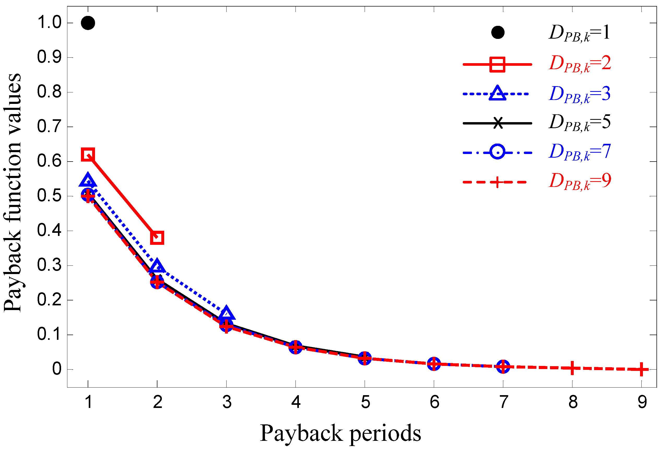
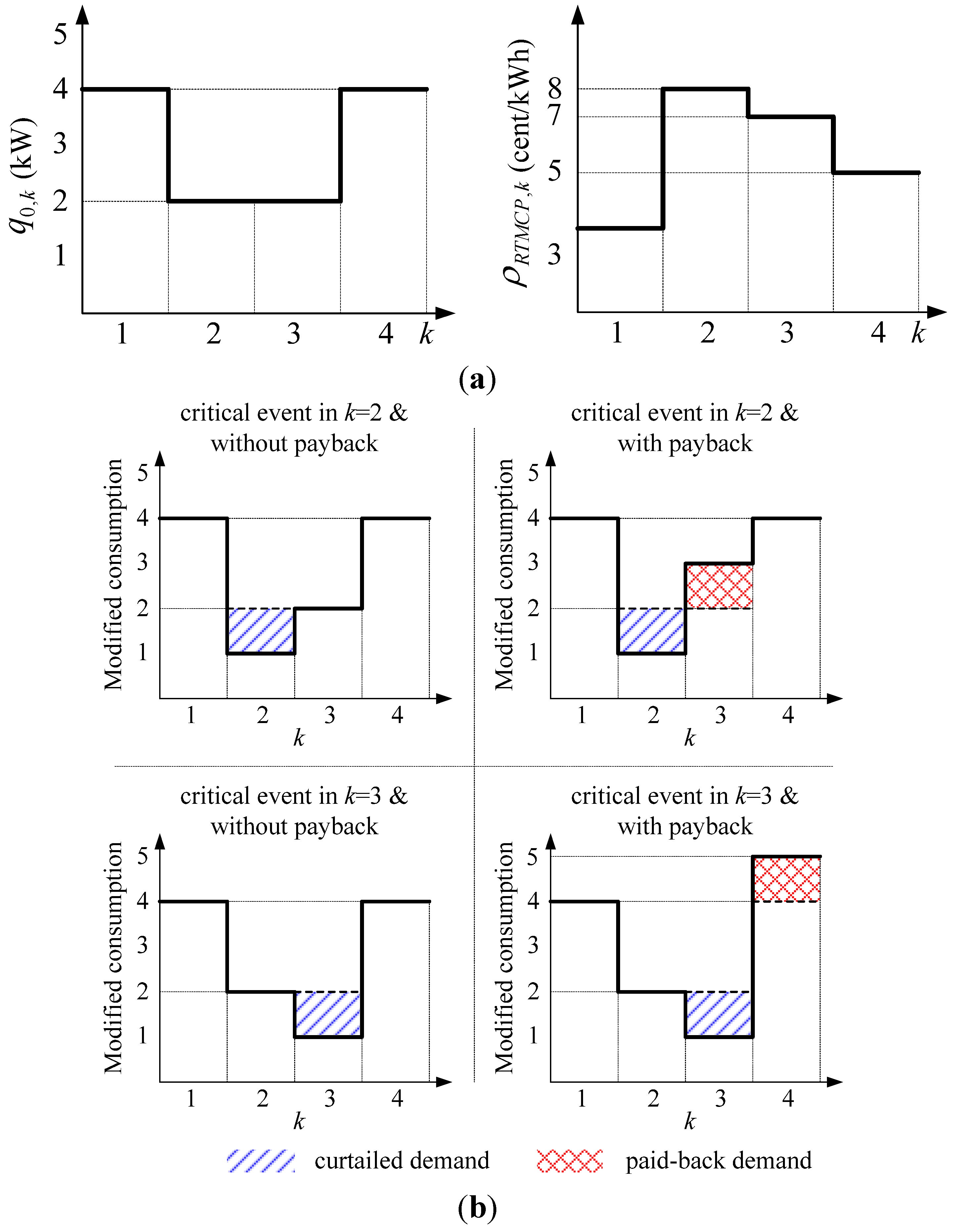
3. Characterization of the Payback Phenomenon

There are two key aspects that characterize the payback phenomenon. The first is the amount of paid-back demand. The curtailed demand, $Q_{CUR,k}$, may be under-, equally, or over-recovered following a critical event [13,14,15]. Thus, a payback ratio, denoted as ${\text{α}}_{PB,k}$, is introduced as the ratio of recovered consumption to curtailed demand. The specific value of ${\text{α}}_{PB,k}$ depends on the composition of customer demand. For example, one does not compensate for turning off lights during a critical event period by greater light use later on; such demand thus tends to be connected with under-payback, or ${\text{α}}_{PB,k}>1$. In contrast, a heating or air-conditioning system may require more post-event energy for transition to the target value from the decreased or increased room temperature arising during the critical event period; this tends to result in over-payback, or ${\text{α}}_{PB,k}>1$. Let $Q_{PB,k}$ be defined as the amount of paid-back demand for a critical event in period k. Then $Q_{PB,k}$ can be represented as:

$$Q_{PB,k}={\displaystyle \sum _{i=k+D_{CPP}}^{k+D_{CPP}+D_{PB,k}-1}{q}_{PB,i}}={\displaystyle \sum _{n=1}^{D_{PB,k}}{q}_{PB,n+k+D_{CPP}-1}}={\text{α}}_{PB,k}{Q}_{CUR,k}$$

(14)

where $q_{PB,i}$ is the recovered demand in period i and ${\text{α}}_{PB,k}$ and $D_{PB,k}$ are the payback ratio and duration, respectively, for the critical event in period k.

The other key aspect of the payback phenomenon is its pattern. Let the payback function, $f_{PB,k}\left(n\right)$ for $n\in \left\{1,2,\cdots ,D_{PB,k}\right\}$, be defined as the ratio of paid-back demand to $Q_{CUR,k}$ in the n-th time period from the end of the critical event. Then, $q_{PB,n+k+D_{CPP}-1}$ in Equation (14) is expressed as:

$$q_{PB,n+k+D_{CPP}-1}=Q_{CUR,k}{f}_{PB,k}(n)$$

(15)

Comparing Equations (14) and (15), $f_{PB,k}\left(n\right)$ should satisfy the condition:

$${\displaystyle \sum _{n=1}^{D_{PB,k}}{f}_{PB,k}(n)}={\text{α}}_{PB,k}$$

(16)

Let the normalized unit payback function, $f_{PB,k}^U\left(n\right)$, be defined as $f_{PB,k}^U\left(n\right)=f_{PB,k}\left(n\right)/{\text{α}}_{PB,k}$, which satisfies the condition:

$${\displaystyle \sum _{n=1}^{D_{PB,k}}{f}_{PB,k}^U(n)}=1$$

(17)

Then, $f_{PB,k}\left(n\right)$ is represented as $f_{PB,k}\left(n\right)={\text{α}}_{PB,k}{f}_{PB,k}^U\left(n\right)$ such that the payback function can be separately expressed by the payback ratio, ${\text{α}}_{PB,k}$, and the payback pattern, $f_{PB,k}^U\text{(}n\text{)}$.

In real-world situations, it is difficult to specify a particular form for $f_{PB,k}^U\text{(}n\text{)}$. Nonetheless, some studies suggest a payback function model for analytic purposes particularly for water heating and air conditioning loads. Empirical results in [14] show that the payback pattern can be represented with an exponentially decreasing function for water heating loads. In [13] and [15], sets of decreasing values are specified as the payback function values for water heating loads and both water heating and air conditioning loads, respectively. This study thus adopts an EDP function as a specific payback pattern to model an intensive recovery of demand over a short time period immediately after a critical event. This takes the form of:

$$f_{PB,k}^U(n)=e^{-n\lambda },n\in \left\{1,2,\cdots ,D_{PB,k}\right\}$$

(18)

where $\lambda$ is a constant, which is determined by solving the equation ${\displaystyle {\sum }_{n=1}^{D_{PB,k}}{e}^{-n\lambda }}=1$ derived from Equation (17). For example, $\lambda =\ln ((1+\sqrt{5})/2)$ can be obtained when $D_{PB,k}=2$. Figure 1 shows the shape of the EDP function for various values of $D_{PB,k}$ when ${\text{α}}_{PB,k}=1$. It should be noted from Figure 1 that the EDP functions are almost identical for $D_{PB,k}$ greater than five.

Figure 1. Exponentially decreasing payback functions for several payback duration values of 1, 2, 3, 5, 7, and 9.

Figure 1. Exponentially decreasing payback functions for several payback duration values of 1, 2, 3, 5, 7, and 9.

Despite past studies [13,14,15] mentioning the EDP pattern, we cannot rule out the possibility that the curtailed demand is recovered fairly evenly during the payback period. Consequently, a constant function is used to model UDP and is analyzed as an additional specific payback pattern for comparison purposes. The UDP function is expressed as:

$$f_{PB,k}^U\text{(}n\text{)}=c,n\in \left\{1,2,\cdots ,D_{PB,k}\right\}$$

(19)

where c is a constant that takes the value $c=1/D_{PB,k}$ from Equation (17).

4. Payback Effects on CPP Design

4.1. Payback Effects on the Event Scheduling Problem

The optimal schedule of critical events that was determined without considering payback may no longer be optimal once the payback phenomenon is taken into account. Further, the LSE’s profits may decrease if the additional costs arising from payback exceed the cost savings reaped through the critical event. A simple example in Figure 2 demonstrates such a scenario. Suppose that $H=4$, $N_{CPP}=1$, $D_{PB,2}=D_{PB,3}=1$, ${\text{α}}_{PB,2}={\text{α}}_{PB,3}=1$, ${\text{ρ}}_{BASE}=4$ cents/kWh, and ${\text{ρ}}_{PEAK}=44$ cents/kWh. The nominal demand and RTMCPs are given in Figure 2a. The customers’ price responsiveness is assumed as $\text{β}=-0.05$.

Under these parameter settings, customers eliminate half of their nominal demand when a critical event is triggered according to Equation (3). Figure 2b and Table 1 present the modified consumption and profit levels under four different scenarios. Without payback, the profit is largest when a critical event is triggered in period $k=2$; when payback is considered, however, the profit-maximizing critical event period shifts to $k=3$. In other words, the optimal event schedule changes due to payback. In addition, profit decreases from $30 in the case without payback to $28 in the case of payback with optimal scheduling. This clearly indicates that payback may have a negative effect on an LSE’s profits, suggesting that the event scheduling problem in the presence of payback must be solved as a separate optimization problem.

Figure 2. (a) Demand and real-time market clearing prices (RTMCPs); (b) A simple example to show how payback affects the optimal schedule of critical events.

Figure 2. (a) Demand and real-time market clearing prices (RTMCPs); (b) A simple example to show how payback affects the optimal schedule of critical events.

Table 1. Profits of the load serving entity (LSE) with and without payback for two event schedules in the example.

Critical Event Period		Without Payback ($)	With Payback ($)
$k=2$	revenue	84	88
	cost	54	61
	profit	30	27
$k=3$	revenue	84	88
	cost	55	60
	profit	29	28

Table 1. Profits of the load serving entity (LSE) with and without payback for two event schedules in the example.

Critical Event Period		Without Payback ($)	With Payback ($)
$k=2$	revenue	84	88
	cost	54	61
	profit	30	27
$k=3$	revenue	84	88
	cost	55	60
	profit	29	28

4.2. Payback Effects on the Optimal Peak Rate

As in Equation (11), the profit index including the payback arising from a critical event in period k, $P{I}_{PB,k}({\text{ρ}}_{PEAK})$, is represented as:

$$\begin{array}{c}P{I}_{PB,k}({\text{ρ}}_{PEAK})={\displaystyle \sum _{i=k}^{k+D_{CPP}-1}\left\{q_{CR,i}\left({\text{ρ}}_{PEAK}-{\text{ρ}}_{RTMCP,i}\right)-q_{0,i}\left({\text{ρ}}_{BASE}-{\text{ρ}}_{RTMCP,i}\right)\right\}}\\ +{\displaystyle \sum _{n=1}^{D_{PB,k}}\left\{{\text{α}}_{PB,k}{Q}_{CUR,k}{f}_{PB,k}^U\left(n\right)\left({\text{ρ}}_{BASE}-{\text{ρ}}_{RTMCP,n+k+D_{CPP}-1}\right)\right\}}\end{array}$$

(20)

As with the procedures for ${\text{ρ}}_{N,PEAK}^{*}$ in Equation (12), the optimal peak rate considering payback, ${\text{ρ}}_{PB,PEAK}^{*}$, can be obtained by substituting Equations (4) into (20), differentiating with respect to ${\text{ρ}}_{PEAK}$, and solving the resulting equation for ${\text{ρ}}_{PEAK}$. After rearranging the terms, a specific form of ${\text{ρ}}_{PB,PEAK}^{*}$ is obtained as:

$$\begin{array}{c}{\text{ρ}}_{PB,PEAK}^{*}=\left[\frac{{\text{ρ}}_{BASE}}{2}\left(1-\frac{1}{\text{β}}\right)+\frac{{\displaystyle \sum _{k\in {{\rm K}}^{*}}{\displaystyle \sum _{i=k}^{k+D_{CPP}-1}{q}_{0,i}{\text{ρ}}_{RTMCP,i}}}}{2{\displaystyle \sum _{k\in {{\rm K}}^{*}}{Q}_{0,k}}}\right]\\ +\left[\frac{{\text{ρ}}_{BASE}{\displaystyle \sum _{k\in {{\rm K}}^{*}}{\text{α}}_{PB,k}{Q}_{0,k}}}{2{\displaystyle \sum _{k\in {{\rm K}}^{*}}{Q}_{0,k}}}-\frac{{\displaystyle \sum _{k\in {{\rm K}}^{*}}\left\{{\text{α}}_{PB,k}{Q}_{0,k}{\displaystyle \sum _{n=1}^{D_{PB,k}}{f}_{PB,k}^U\left(n\right){\text{ρ}}_{RTMCP,n+k+D_{CPP}-1}}\right\}}}{2{\displaystyle \sum _{k\in {{\rm K}}^{*}}{Q}_{0,k}}}\right]\end{array}$$

(21)

The terms in the first square bracket in Equation (21) are equal to ${\text{ρ}}_{N,PEAK}^{*}$ in Equation (12). Thus, ${\text{ρ}}_{PB,PEAK}^{*}$ can be represented as:

$${\text{ρ}}_{PB,PEAK}^{*}={\text{ρ}}_{N,PEAK}^{*}+\Delta {\text{ρ}}_{PB,PEAK}$$

(22)

where $\Delta {\text{ρ}}_{PB,PEAK}$ indicates the payback effect on the optimal peak rate, the expression of which is as given in the second bracket in Equation (21). The optimal event schedule, ${{\rm K}}^{*}$, depends on ${\text{α}}_{PB}$. Thus, ${\text{α}}_{PB}$ should be included within the summation sign in Equation (21). However, if ${{\rm K}}^{*}$ does not change and the payback parameters are the same for $k\in {{\rm K}}^{*}$, that is, ${\text{α}}_{PB,k}={\text{α}}_{PB}$, $D_{PB,k}=D_{PB}$, and $f_{PB,k}^U\left(n\right)=f_{PB}^U\left(n\right)$ for $k\in {{\rm K}}^{*}$, then ${\text{α}}_{PB}$ can be pulled out of the sum and $\Delta {\text{ρ}}_{PB,PEAK}$ can be represented as:

$$\Delta {\text{ρ}}_{PB,PEAK}=\frac{{\text{α}}_{PB}}{2}\left\{{\text{ρ}}_{BASE}-\frac{{\displaystyle \sum _{k\in {{\rm K}}^{*}}\left\{Q_{0,k}{\displaystyle \sum _{n=1}^{D_{PB}}{f}_{PB}^U\left(n\right){\text{ρ}}_{RTMCP,n+k+D_{CPP}-1}}\right\}}}{{\displaystyle \sum _{k\in {{\rm K}}^{*}}{Q}_{0,k}}}\right\}$$

(23)

Equation (23) shows that, while maintaining the optimal schedule of critical events, the payback ratio, ${\text{α}}_{PB}$, has a linear relationship with the amount of change in the optimal peak rate. ${\text{α}}_{PB}$ is not, however, related to whether the payback causes an increase or decrease in the optimal peak rate. On the other hand, the payback pattern, $f_{PB}^U\left(n\right)$, and duration, $D_{PB}$, affect both the amount and sign of the change in the optimal peak rate.

Despite the relationships between the payback parameters and the optimal peak rate, it is not evident whether payback causes an increase or decrease in the optimal peak rate based only on Equation (23). This is because $\Delta {\text{ρ}}_{PB,PEAK}$ depends on the specific RTMCPs and nominal demand as well as the payback parameters; the interrelation among these factors is difficult to define conclusively, particularly in cases where $N_{CPP}\ge 2$. As a result, the payback effects on the optimal peak rate will first be examined analytically for the simplest case ($N_{CPP}=1$). These results will then be extrapolated to the general cases with $N_{CPP}\ge 2$.

Suppose that $N_{CPP}=1$ and the optimal event schedule is determined as ${{\rm K}}^{*}=\text{{}{k}^{*}\text{}}$. Then, $Q_{0,k}$ terms in the numerator and denominator of Equation (23) cancel one another out and $\Delta {\text{ρ}}_{PB,PEAK}$ can be simplified to:

$$\Delta {\text{ρ}}_{PB,PEAK}=\frac{{\text{α}}_{PB}}{2}\left\{{\text{ρ}}_{BASE}-{\displaystyle \sum _{n=1}^{D_{PB}}{f}_{PB}^U\left(n\right){\text{ρ}}_{RTMCP,n+k^{*}+D_{CPP}-1}}\right\}$$

(24)

For EDP, most of the paid-back demand is concentrated in the initial time periods following the critical event. In addition, a critical event is usually triggered when the real-time market clearing price (RTMCP) is high, such that the RTMCPs in the early time periods of the payback phase are likely to be higher than ${\text{ρ}}_{BASE}$. This implies that the second term inside the bracket in Equation (24), which refers to the average RTMCP weighed by $f_{PB}^U\left(n\right)$ during the payback periods, is also likely to exceed ${\text{ρ}}_{BASE}$; $\Delta {\text{ρ}}_{PB,PEAK}$ is thus negative. Consequently, for EDP, where the curtailed demand is recovered quickly, ${\text{ρ}}_{PB,PEAK}^{*}$ tends to be lower than ${\text{ρ}}_{N,PEAK}^{*}$. Additionally, as described in Section 3, the EDP functions hardly change for $D_{PB}\ge 5$. Therefore, for EDP, as $D_{PB}$ increases, ${\text{ρ}}_{PB,PEAK}^{*}$ converges to a value, which is likely less than ${\text{ρ}}_{N,PEAK}^{*}$.

For UDP, $\Delta {\text{ρ}}_{PB,PEAK}$ in Equation (24) can be simplified as:

$$\Delta {\text{ρ}}_{PB,PEAK}=\frac{{\text{α}}_{PB}}{2}\left\{{\text{ρ}}_{BASE}-\frac{1}{D_{PB}}{\displaystyle \sum _{n=1}^{D_{PB}}{\text{ρ}}_{RTMCP,n+k^{*}+D_{CPP}-1}}\right\}$$

(25)

In Equation (25), all relevant RTMCPs are equally weighted in the calculation of $\Delta {\text{ρ}}_{PB,PEAK}$. In addition, the RTMCPs are likely to be small, as the times in question are far from the critical event period. As a result, the absolute value of $\Delta {\text{ρ}}_{PB,PEAK}$ for UDP might be smaller than for EDP, suggesting that ${\text{ρ}}_{PB,PEAK}^{*}$ is greater for UDP than for EDP. In the extreme situation when the RTMCPs below ${\text{ρ}}_{BASE}$ are dominant over a long payback duration, it is possible that $\Delta {\text{ρ}}_{PB,PEAK}$ becomes positive and thus ${\text{ρ}}_{PB,PEAK}^{*}$ exceeds ${\text{ρ}}_{N,PEAK}^{*}$. Moreover, assuming that ${\text{ρ}}_{BASE}$ is set close to the average of the RTMCPs over all periods, ${\text{ρ}}_{PB,PEAK}^{*}$ for UDP approaches ${\text{ρ}}_{N,PEAK}^{*}$ as the payback duration increases. Nonetheless, in real situations, the payback duration is usually limited to a few time periods, and the RTMCPs around the critical event periods are likely to exceed ${\text{ρ}}_{BASE}$. Therefore, ${\text{ρ}}_{PB,PEAK}^{*}$ for UDP is still likely to be below ${\text{ρ}}_{N,PEAK}^{*}$, even though it increases and approaches ${\text{ρ}}_{N,PEAK}^{*}$ as the payback duration increases.

Until now, the analysis has considered payback effects on the optimal peak rate for the simplest case, $N_{CPP}=1$. As indicated in Equation (23), $\Delta {\text{ρ}}_{PB,PEAK}$ in the general case $N_{CPP}\ge 2$) can be interpreted as a superposition of the effects for the $N_{CPP}=1$ case, weighted by the $Q_{0,k}$ terms. In other words, $\Delta {\text{ρ}}_{PB,PEAK}$ for $N_{CPP}\ge 2$ can be determined as the weighted sum of $N_{CPP}$ terms of $\Delta {\text{ρ}}_{PB,PEAK}$ for $N_{CPP}=1$. Therefore, the above-presented analysis of payback effects on the optimal peak rate remains valid in cases with $N_{CPP}\ge 2$ unless $Q_{0,k}$ takes a very abnormal value for a certain critical event. Nonetheless, the payback effects on the optimal peak rate still depend strongly on the specific conditions of the RTMCPs and demand levels. As a result, the following section will perform numerical simulations for $N_{CPP}=3$ given specific values of the RTMCP and demand; this will allow verification of the payback effects for $N_{CPP}=1$ and validate their application to cases with $N_{CPP}\ge 2$.

5. Simulations and Verification

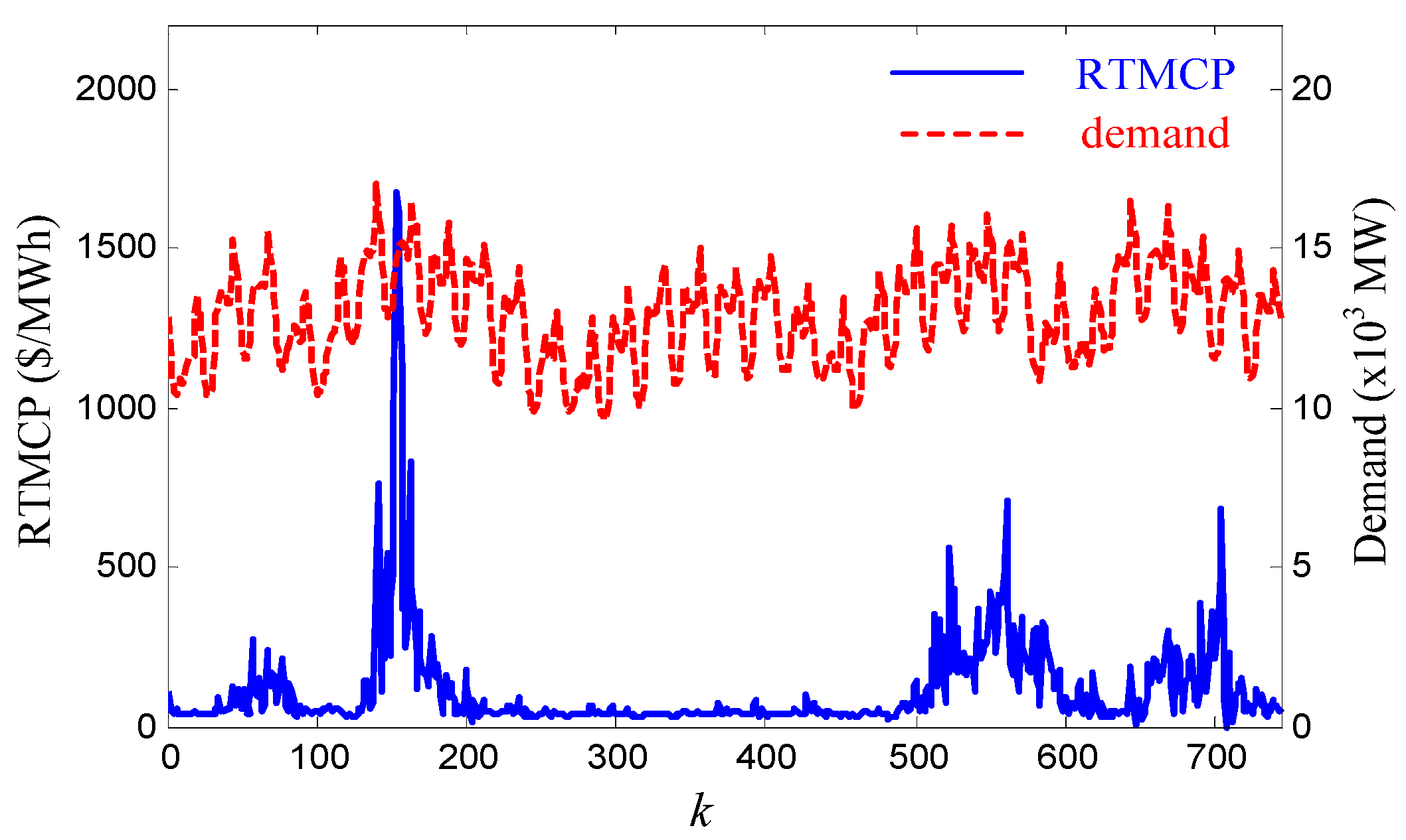
5.1. Simulation Methods

Actual data for future RTMCPs and demand is unavailable when an LSE designs a CPP scheme. Thus, these quantities must be forecasted for all periods within the scheduling time horizon. In this study’s simulations, the autoregressive moving average (ARMA) method in [24] is used for the forecasting. Historical data on RTMCPs and demand levels, as announced by the Pennsylvania-New Jersey-Maryland Interconnection for 31 days in January 2014 [25], are used as input data for the ARMA method. The resulting forecasted data are shown in Figure 3. The time period length is assumed to be one hour, making the simulations’ scheduling time horizon, H, equal to 744. The simulations are performed using the CPP parameters of $N_{CPP}=3$, $\Delta k=48$ hours, and ${\text{ρ}}_{BASE}=12$ cents/kWh and a customer price responsiveness of $\text{β}=-0.05$. It is assumed that the payback parameters are equal for all critical event time period, that is, ${\text{α}}_{PB,k}={\text{α}}_{PB}$, $D_{PB,k}=D_{PB}$, and $f_{PB,k}^U\left(n\right)=f_{PB}^U\left(n\right)$.

Figure 3. Forecasted data for real-time market clearing price (RTMCP) and demand.

Figure 3. Forecasted data for real-time market clearing price (RTMCP) and demand.

5.2. Results: Payback Effects on the Optimal Event Schedule

The effects of payback on the event scheduling problem are examined under the conditions that ${\text{α}}_{PB}=1$ and $D_{PB}=3$ h. For set-ups both with and without payback, the optimal peak rate is arbitrarily selected as ${\text{ρ}}_{N,PEAK}={\text{ρ}}_{PB,PEAK}=120$ cents/kWh. Simulations of three different scenarios were undertaken, as listed in Table 2, including without payback, with EDP, and with UDP. The specific values of the payback functions are also given in Table 2 (first column).

The results for the simulated optimal schedule and corresponding profits are also listed in Table 2. The optimal schedules differ from one another according to not only whether or not payback occurs but also the payback pattern. This suggests that the payback phenomenon must be considered to properly solve the event scheduling problem. Furthermore, the profit is larger in the non-payback case than in either case with payback, verifying that the payback phenomenon has a negative effect on the LSE’s profits due to the additional cost of the paid-back demand.

Table 2. Simulation results for the optimal schedule and the corresponding profit of the LSE.

$f_{PB}\text{(}n\text{)}=\left\{f_{PB}\text{(}1\text{)},f_{PB}\text{(}2\text{)},f_{PB}\text{(}3\text{)}\right\}$	Optimal Schedule of Critical Events	Profit (Million Dollars)
Without payback	{154, 561, 668}	46.476
Exponentially decreasing payback {0.54, 0.30, 0.16}	{157, 561, 644}	40.265
Uniformly distributed payback {1/3, 1/3, 1/3}	{157, 561, 704}	40.843

Table 2. Simulation results for the optimal schedule and the corresponding profit of the LSE.

$f_{PB}\text{(}n\text{)}=\left\{f_{PB}\text{(}1\text{)},f_{PB}\text{(}2\text{)},f_{PB}\text{(}3\text{)}\right\}$	Optimal Schedule of Critical Events	Profit (Million Dollars)
Without payback	{154, 561, 668}	46.476
Exponentially decreasing payback {0.54, 0.30, 0.16}	{157, 561, 644}	40.265
Uniformly distributed payback {1/3, 1/3, 1/3}	{157, 561, 704}	40.843

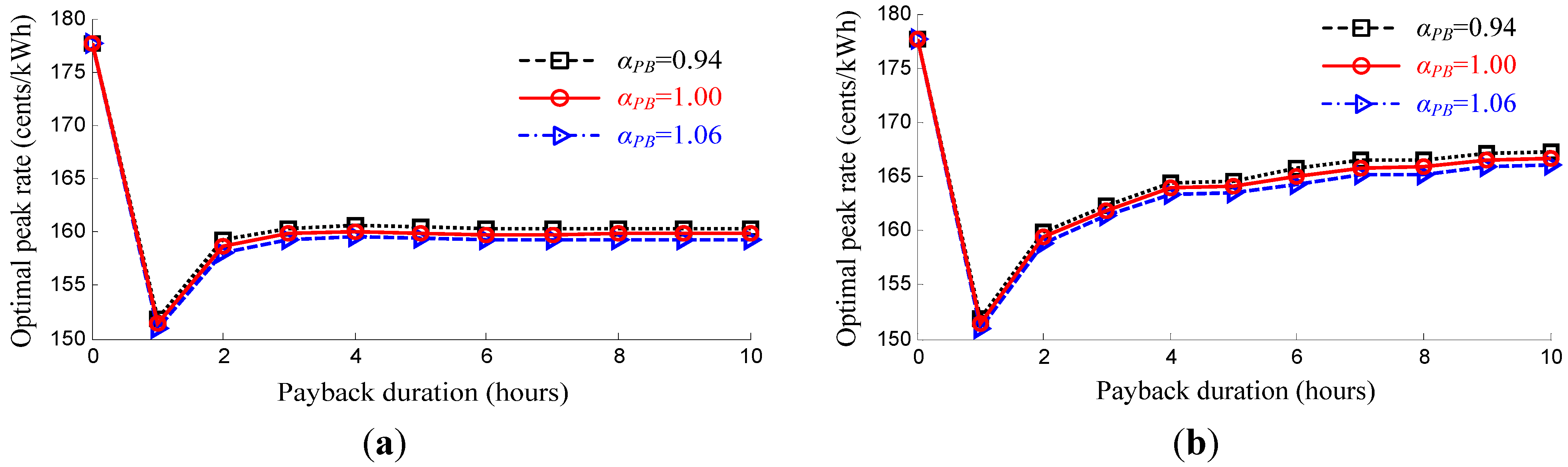
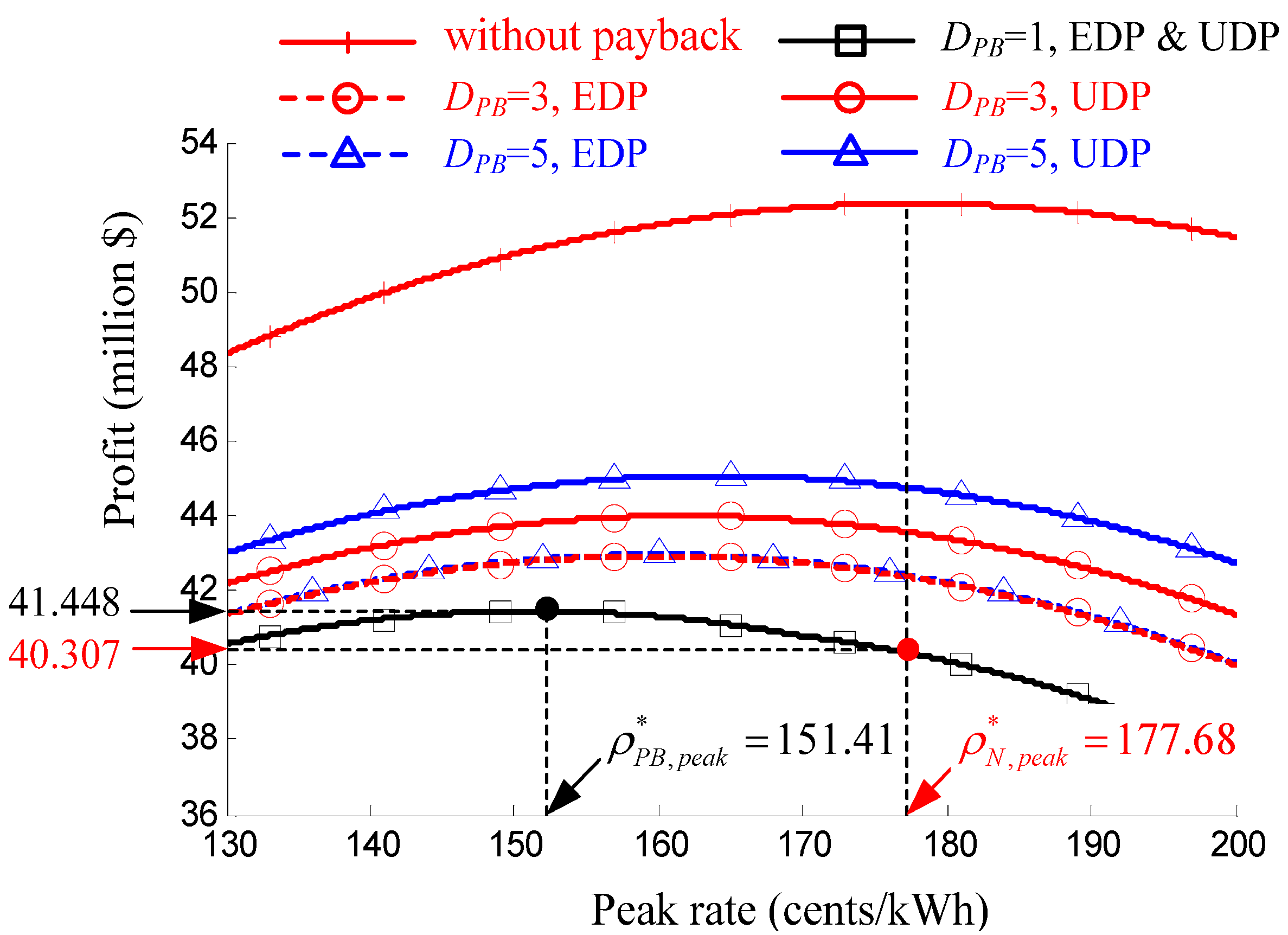
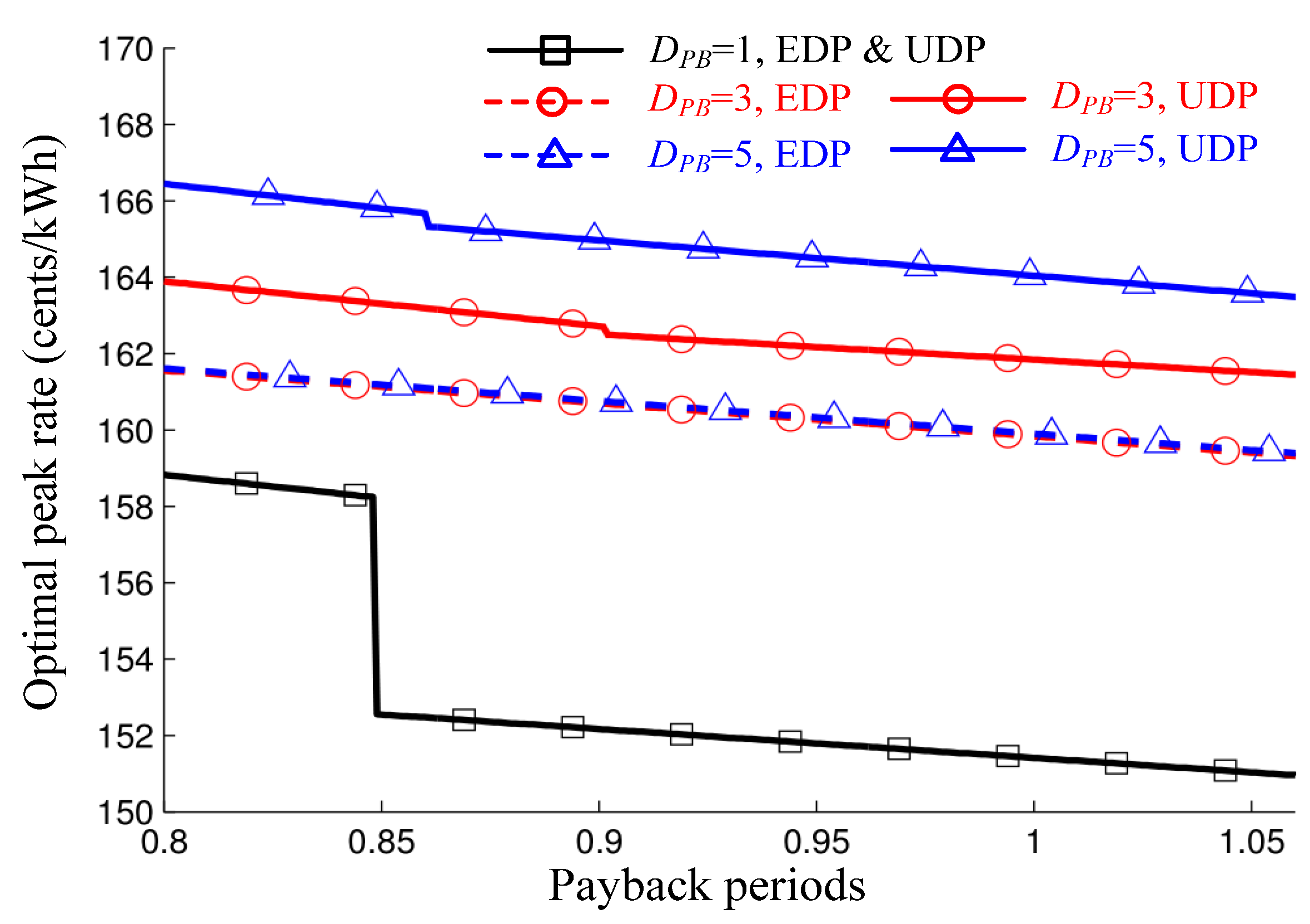
5.3. Result: Payback Effects on the Optimal Peak Rate

The effects of payback on the optimal peak rate are simulated by changing the payback duration and ratio. The payback duration is set to change from one to ten ($D_{PB}\in \text{{}1,2,\cdots ,10\text{}}$), and the range of the payback ratio is taken from [13] as $0.80\le {\text{α}}_{PB}\le 1.06$, with 271 equidistant values of ${\text{α}}_{PB}$ selected within this range. For each combination of $D_{PB}$ and ${\text{α}}_{PB}$, the optimal peak rate is determined from Equation (21) and the corresponding profit for the LSE is calculated. For the case without payback, we find that ${\text{ρ}}_{N,PEAK}^{*}=177.68$ (cents/kWh), which yields a profit of $52.355 million.

The simulation results for the optimal peak rate, ${\text{ρ}}_{PB,PEAK}^{*}$, for three values of ${\text{α}}_{PB}$ are presented with respect to ${\text{α}}_{PB}$ in Figure 4, where $D_{PB}=0$ indicates the case without payback. As described in Section 4.2, the values of ${\text{ρ}}_{PB,PEAK}^{*}$ are below ${\text{ρ}}_{N,PEAK}^{*}$ in all simulations because the RTMCP values around critical event periods are larger than ${\text{ρ}}_{BASE}$. Therefore, ${\text{ρ}}_{PB,PEAK}^{*}$ should be set below the usual level if the payback phenomenon is expected. In addition, Figure 4 shows that ${\text{ρ}}_{PB,PEAK}^{*}$ tends to be smaller for a short payback duration than for a long one, regardless of the payback pattern. This suggests that the LSE should select a lower optimal peak rate if the payback period is expected to be short.

Figure 4 also demonstrates how the payback pattern affects the optimal peak rate. The value of ${\text{ρ}}_{PB,PEAK}^{*}$ is smaller for EDP than for UDP, particularly for a long payback duration. This is because the RTMCPs in the late time periods of the payback duration are smaller than those in the early time periods, but they are all equally weighted when determining ${\text{ρ}}_{PB,PEAK}^{*}$ for UDP. Moreover, in contrast with the fact that ${\text{ρ}}_{PB,PEAK}^{*}$ for UDP increases as $D_{PB}$ increases, ${\text{ρ}}_{PB,PEAK}^{*}$ for EDP hardly changes for $D_{PB}\ge 5$.

As shown in Figure 4, the effect of ${\text{α}}_{PB}$ on the changing shape of ${\text{ρ}}_{PB,PEAK}^{*}$ is insignificant when compared with the effect of $D_{PB}$. Nevertheless, to examine the effects of ${\text{α}}_{PB}$ on ${\text{ρ}}_{PB,PEAK}^{*}$ in greater detail, the change in ${\text{ρ}}_{PB,PEAK}^{*}$ with respect to ${\text{α}}_{PB}$ is represented in Figure 5 for a few values of $D_{PB}$. As Equation (24) and the associated analyses indicate, ${\text{ρ}}_{PB,PEAK}^{*}$ decreases linearly as ${\text{α}}_{PB}$ increases, irrespective of the payback duration and pattern. This linear relationship between ${\text{α}}_{PB}$ and ${\text{ρ}}_{PB,PEAK}^{*}$ holds only as long as the optimal event schedule, ${{\rm K}}^{*}$, does not change. When the optimal schedule changes, a step change of ${\text{ρ}}_{PB,PEAK}^{*}$ occurs, as can be clearly observed from the cases $D_{PB}=1$ for EDP and UDP and $D_{PB}=5$ for UDP in Figure 5. However, Figure 5 shows that ${\text{ρ}}_{PB,PEAK}^{*}$ decreases linearly after the step change as long as the modified optimal schedule is maintained.

Figure 4. Simulation results of the optimal peak rate with respect to the payback duration for (a) Exponentially decreasing payback (EDP); (b) Uniformly distributed payback (UDP).

Figure 4. Simulation results of the optimal peak rate with respect to the payback duration for (a) Exponentially decreasing payback (EDP); (b) Uniformly distributed payback (UDP).

Figure 5. Simulation results of the optimal peak rate with respect to the payback ratio for selected values of $D_{PB}$.

Figure 5. Simulation results of the optimal peak rate with respect to the payback ratio for selected values of $D_{PB}$.

Finally, it is necessary to check whether the values of ${\text{ρ}}_{PB,PEAK}^{*}$ determined in the simulations are optimal. Figure 6 illustrates the profits with payback for $D_{PB}\in \text{{}1,3,5\text{}}$ and ${\text{α}}_{PB}=1$ with respect to the peak rate for the two payback patterns. The profit without payback is also shown in Figure 6. The values for ${\text{ρ}}_{N,PEAK}^{*}$ and ${\text{ρ}}_{PB,PEAK}^{*}$ determined via the simulation are clearly the extreme ones, yielding maximum profits. The existence of payback decreases profits in all cases. To emphasize the significance of this analysis, the profits resulting when ${\text{ρ}}_{N,PEAK}^{*}=177.68$ cents/kWh and ${\text{ρ}}_{PB,PEAK}^{*}=151.41$ cents/kWh for $D_{PB}=1$ and ${\text{α}}_{PB}=1$ are indicated in Figure 6. (Note that the functions for the two payback patterns are the same for $D_{PB}=1$). Comparing the two profits reveals that using ${\text{ρ}}_{PB,PEAK}^{*}$ increases profits by 2.83% (from $40.307 million for ${\text{ρ}}_{N,PEAK}^{*}$ to $41.448 million for ${\text{ρ}}_{PB,PEAK}^{*}$). In practical terms, properly designing a CPP scheme by considering payback effects could lead to a significant, if not dramatic, increase in profits for the LSE.

Figure 6. Profit of the load serving entities (LSE) with respect to the peak rate for the case without payback and several cases with payback.

Figure 6. Profit of the load serving entities (LSE) with respect to the peak rate for the case without payback and several cases with payback.

6. Conclusions

A CPP scheme is a useful demand response program that enables an LSE to increase profits by controlling customers’ demand at key moments. However, these profits are later reduced by the payback phenomenon. This study considered optimal strategies for designing a profit-maximizing CPP scheme taking payback into consideration. After characterizing payback through the appropriate parameters, the resulting change in optimal event scheduling was demonstrated, and the optimal peak rate under payback was analytically derived. The validity of this analysis was then verified through numerical simulations.

The results yield certain practical suggestions for designing a CPP scheme in a payback scenario. When payback occurs, it is better to set the peak rate to a lower value than would be optimal without payback. Moreover, if the paid-back demand is expected to be concentrated in the time periods soon after a critical event, the peak rate should be set at an even lower value. As long as the optimal event schedule does not change, payback results in a slight linear decrease in the optimal peak rate. However, if the schedule changes, there is a step change in the optimal peak rate. Consequently, the LSE should jointly optimize the event schedule and the peak rate.

Although the results of the proposed method are helpful for designing a CPP scheme, there remain open questions regarding their practical applications. In particular, the availability of payback parameters, which are not constant but depend on the levels of demand and price, can be challenging in the implementation of a CPP scheme. This is one reason why payback has never been considered in the operation of a real-world CPP scheme; as such, it is not obvious that the extended characterization of the payback concept with other unknown and arbitrary parameters will have meaningful implications for actual operations. Additionally, the effects of nonlinear and unpredictable behavior resulting from different compositions of customer loads need to be examined. Therefore, further empirical research will be necessary to demonstrate the practical implications and real-world effectiveness of the CPP design strategy presented here.

References

1. U.S. Department of Energy. Benefits of Demand Response in Electricity Markets and Recommendations for Achieving Them: A Report to the United States Congress; U.S. Department of Energy: Washington, DC, USA, 2006.
2. Kirschen, D.S. Demand-side view of electricity markets. IEEE Trans. Power Syst. 2003, 18, 520–527. [Google Scholar] [CrossRef]
3. Doostizadeh, M.; Ghasemi, H. A day-ahead electricity pricing model based on smart metering and demand-side management. Energy 2012, 46, 221–230. [Google Scholar] [CrossRef]
4. Ferrero, R.W.; Rivera, J.F.; Shahidehpour, S.M. Application of games with incomplete information for pricing electricity in deregulated power pools. IEEE Trans. Power Syst. 1998, 13, 184–189. [Google Scholar] [CrossRef]
5. Kirschen, D.S.; Strbac, G. Fundamentals of Power System Economics; John Wiley & Sons: Chichester, UK, 2004; pp. 75–79. [Google Scholar]
6. Albadi, M.H.; El-Saadany, E.F. A summary of demand response in electricity markets. Elect. Power Syst. Res. 2008, 78, 1989–1996. [Google Scholar] [CrossRef]
7. Herter, K. Residential implementation of critical peak pricing of electricity. Energy Policy 2007, 35, 2121–2130. [Google Scholar] [CrossRef]
8. Joo, J.-Y.; Ahn, S.H.; Yoon, Y.T.; Choi, J.W. Option valuation applied to implementing demand response via critical peak pricing. In Proceedings of the IEEE PES General Meeting, Tampa, FL, USA, 24–28 June 2007; pp. 1–7.
9. Chen, W.; Wang, X.; Petersen, J.; Tyagi, R.; Black, J. Optimal scheduling of demand response events for electric utilities. IEEE Trans. Smart Grid 2013, 4, 2309–2319. [Google Scholar] [CrossRef]
10. Zhang, Q.; Wang, X.; Fu, M. Optimal implementation strategies for critical peak pricing. In Proceedings of the 6th International Conference on the European Energy Market (EEM), Leuven, Belgium, 27–29 May 2009; pp. 1–6.
11. Park, S.C.; Jin, Y.G.; Song, H.Y.; Yoon, Y.T. Designing a critical peak pricing scheme for the profit maximization objective considering price responsiveness of customers. Energy 2015, 83, 521–531. [Google Scholar] [CrossRef]
12. Zhang, X. Optimal scheduling of critical peak pricing considering wind commitment. IEEE Trans. Sustain. Energy 2014, 5, 637–645. [Google Scholar] [CrossRef]
13. Wei, D.; Chen, N. Air conditioner direct load control by multi-pass dynamic programming. IEEE Trans. Power Syst. 1995, 10, 307–313. [Google Scholar]
14. Ericson, T. Direct load control of residential water heaters. Energy Policy 2009, 37, 3502–3512. [Google Scholar] [CrossRef]
15. Cohen, A.I.; Patmore, J.W.; Oglevee, D.H.; Berman, R.W.; Ayers, L.H.; Howard, J.F. An integrated system for residential load control. IEEE Trans. Power App. Syst. 1987, 2, 645–651. [Google Scholar] [CrossRef]
16. Nguyen, D.T.; Negnevitsky, M.; de Groot, M. Modeling load recovery impact for demand response applications. IEEE Trans. Power Syst. 2013, 28, 1216–1225. [Google Scholar] [CrossRef]
17. Karangelos, E.; Bouffard, F. Towards full integration of demand-side resources in joint forward energy/reserve electricity markets. IEEE Trans. Power Syst. 2012, 27, 280–289. [Google Scholar] [CrossRef]
18. Kirschen, D.S.; Strbac, G.; Cumperayot, P.; de Paiva Mendes, D. Factoring the elasticity of demand in electricity. IEEE Trans. Power Syst. 2000, 15, 612–617. [Google Scholar] [CrossRef]
19. Strbac, G. Demand side management: Benefits and challenges. Energy Policy 2008, 36, 4419–4426. [Google Scholar] [CrossRef]
20. Shaw, R.; Attree, M.; Jackson, T.; Kay, M. The value of reducing distribution losses by domestic load-shifting: A network perspective. Energy Policy 2009, 37, 3159–3167. [Google Scholar] [CrossRef]
21. Strbac, G.; Kirschen, D.S. Assessing the competitiveness of demand-side bidding. IEEE Trans. Power Syst. 1999, 14, 120–125. [Google Scholar] [CrossRef]
22. Piette, M.A.; Watson, D.; Motegi, N.; Kiliccote, S. Automated Critical Peak Pricing Field Tests: 2006 Pilot Program Description and Results; Lawrence Berkeley National Laboratory: Berkeley, CA, USA, 2007. [Google Scholar]
23. Schweppe, F.C.; Caramanis, M.C.; Tabors, R.D.; Bohn, R.E. Spot Pricing of Electricity; Springer: New York, NY, USA, 1988; pp. 327–333. [Google Scholar]
24. Weron, R. Modeling and Forecasting Electricity Loads and Prices: A Statistical Approach; John Wiley & Sons: Chichester, UK, 2007; pp. 84–85; 109–110. [Google Scholar]
25. PJM Market & Operations: Real-time Energy Market Data. Available online: http://www.pjm.com/markets-and-operations/energy/real-time.aspx (accessed on 14 February 2015).