Short-Term Electrical Peak Demand Forecasting in a Large Government Building Using Artificial Neural Networks


Abstract
: The power output capacity of a local electrical utility is dictated by its customers' cumulative peak-demand electrical consumption. Most electrical utilities in the United States maintain peak-power generation capacity by charging for end-use peak electrical demand; thirty to seventy percent of an electric utility's bill. To reduce peak demand, a real-time energy monitoring system was designed, developed, and implemented for a large government building. Data logging, combined with an application of artificial neural networks (ANNs), provides short-term electrical load forecasting data for controlled peak demand. The ANN model was tested against other forecasting methods including simple moving average (SMA), linear regression, and multivariate adaptive regression splines (MARSplines) and was effective at forecasting peak building electrical demand in a large government building sixty minutes into the future. The ANN model presented here outperformed the other forecasting methods tested with a mean absolute percentage error (MAPE) of 3.9% as compared to the SMA, linear regression, and MARSplines MAPEs of 7.7%, 17.3%, and 7.0% respectively. Additionally, the ANN model realized an absolute maximum error (AME) of 8.2% as compared to the SMA, linear regression, and MARSplines AMEs of 26.2%, 45.1%, and 22.5% respectively.1. Introduction
The U.S. Department of Energy's modern grid initiative states that a “smart grid” integrates advanced sensing technologies, control methods, and integrated communications into the existing electricity grid [1]. A critical component of the smart grid with distributed generation is peak demand forecasting. Given accurate, real-time electrical demand information, power utilities are able to meet demand more efficiently by building appropriately sized power plants and support infrastructure. Real-time demand information reduces energy wastage, thereby lessening the overall environmental impact of energy conversion. As total electrical demand continues to increase with energy sources becoming less abundant and affordable, the overall sustainability of meeting aggregate end-user electrical demand depends greatly on the efficient usage of all available energy conversion.
An electrical utility's demand charge, measured in kilowatts (kW), is the price charged for the peak amount of power demanded/consumed at a particular instant by an end-user during one billing cycle. The kW demand charge is not to be confused with the more commonly known utility's power consumption charge, which is the amount of power consumed over a period of time; otherwise referred to as kilowatt hours (kWh). The kW demand charge, commonly incurred by large buildings, industrial and commercial complexes, and large manufacturers but more recently also being incorporated into modern residential pricing structures, is the measurement of peak power demanded/consumed at a particular moment during one billing cycle. For most utilities, kW demand is metered throughout the billing cycle in 15 or 30 min intervals. Demand-related charges represent anywhere from 30% to 70% of most commercial and industrial customers' electric bills.
Existing peak-demand forecasting research literature focuses primarily on the utility conversion level for aggregate demand. This research, however, aims to further develop as well as complement existing peak demand forecasting methodologies in an effort to better understand and control peak-demand occurrences experienced not only by the power utilities but more specifically by the end-user.
Demand Side Management (DSM), Demand Response (DR), and/or load management all pertain to the management and actions of electrical end-use behavior [2,3]. When a utility experiences high demand, these load management programs facilitate system load balancing by avoiding peak occurrences [4]. DR has been gaining prominence in recent years as an effective inexpensive tool for reducing overall experienced utility peak demand while improving system-wide energy system efficiency [5]. Through the curtailment of electricity consumed by end-users during periods of high demand or electricity grid instability, DR technology addresses unexpected variances in electricity supply and demand levels. When wholesale electricity market prices are high or when overall grid system reliability is compromised, DR programs offer incentives to end-users in order to affect time of use, instantaneous demand level, and/or aggregate electricity consumption [6]. Additionally, global adaptation and implementation of DR has been documented [7].
Demand response is categorized into two groups: price-based and incentive-based DR [8,9]. With time-of-use (TOU), real-time pricing (RTP), and critical-peak pricing (CPP) rate structures, price-based DR motivates customers to alter their consumption in response to fluctuations in their purchase prices. By shifting consumption from periods of higher energy prices to periods of lower energy prices, end users can reduce their energy cost. Price-based DR is, however, entirely voluntary. Incentive-based demand response, rather, involves fixed or fluctuating time incentives coupled with defined electricity rates. All players, including the district grid operators, load-serving entities, and/or utilities, dictate such incentives. End-users that fail to respond during a peak event in a manner previously agreed upon are penalized financially. There are six typical incentive-based DR programs: Direct Load Control (DLC), Interruptible/Curtailable Service (ICS), Demand Bidding/Buyback (DBB), Emergency Demand Response (EDR), Capacity Market (CM), and Ancillary Services Market (ASM) [2].
Currently, there are several univariate time series and casual exogeneous factors models for short-term (minutes to days ahead) electrical load forecasting: multiplicative autoregressive models, dynamic linear or nonlinear models, threshold autoregressive models, Kalman filtering methods, Box and Jenkins transfer functions, ARMAX models, optimization techniques, nonparametric regression, structural models, and curve-fitting procedures [10]. In addition to these established models and in the past few decades, however, ANNs, similar to fuzzy inference and fuzzy-neural models, have been applied to the load forecasting problem [11–14]. As opposed to traditional computational programs, ANNs provide an adaptive learning approach to predicting future peak demand allowing for more flexibility with new and/or unknown data patterns. Several utilities have even implemented ANNs into operational general practice [15].
ANNs attempt to simulate complex biological neural networks via advanced data manipulation. In a neural network, learning occurs when the network adjusts itself in response to a stimulus in an effort to produce a valued response. Being a continuous classification process, a stimulus is both recognized and matched to a current classification in the network or if it is not recognized, a new classification set is created. An ANN learns dynamically and responds to a stimulus by adjusting its synaptic weights in an effort to make the output response converge towards the anticipated response. In an ANN, learning has thus occurred and knowledge gained when actual response equals the anticipated response.
The leading characteristic of neural and adaptive systems is their adaptability. Rather than being derived by specification, neural and adaptive systems use external data to automatically set their parameters [16]. This means that neural systems are parametric. It also means that they are made “aware” of their output through a performance feedback loop that includes a cost function. The performance feedback is utilized directly to change the parameters through systematic procedures called learning or training rules, so that the system output improves with respect to the desired goal [16].
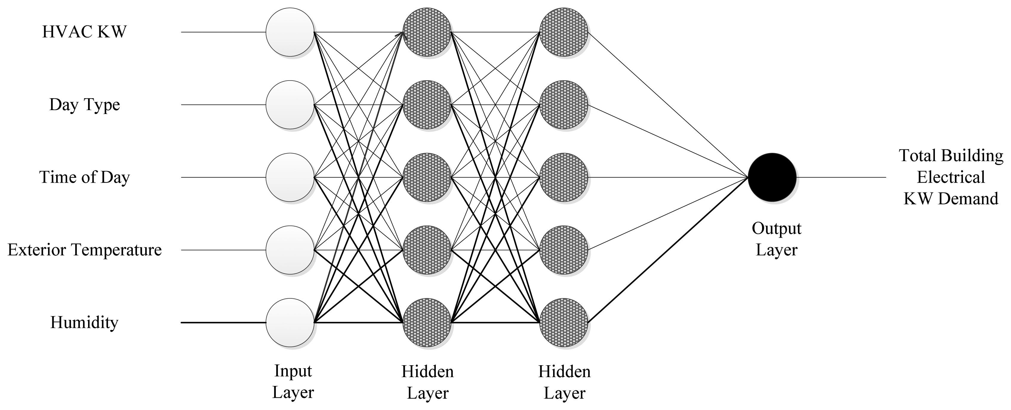
With ANNs, a feed-forward (typical) non-linear dynamic system must be specified, numerical training samples that are adequately represented must be assimilated, and training samples must be encoded in the dynamic system via multiple rounds of repetitive learning [17]. The ANN proposed here uses heating ventilation and air-conditioning (HVAC) electrical consumption, type of day, time of day, outdoor temperature, and humidity as inputs with total building electrical demand as its output.
The research presented in this paper focuses primarily to augment current ICS DR programs by giving localized peak-demand forecasting of the end-user to the end-user. Currently ICS DR is initiated based on utility side supply constraints in an effort to better manage total system-wide peak power production capability. This research, however, fosters a real-time approach to curtailment whereby action is taken by the end-user when forward predicted demand by the end-user approaches some predetermined peak. Such action would thereby empower the end-user to lessen their overall peak-demand and its corresponding cost during each billing cycle.
The goal of this paper is to develop a new method for forecasting peak demand in large buildings using ANNs and a specified period of training days. The approach is intended for medium to large-scale building systems, including government and corporate building campuses, where overall forward demand knowledge is of interest in order to facilitate effective and efficient building electrical utilization and loading. A developed real-time electrical monitoring system prototype capable of forecasting using ANNs is applied to a large government building.
The paper is organized as follows: Section 2 presents the description of the building. Section 3 details the methodology including the data collection system design (hardware, software, and measurement and verification) as well as the proposed ANN architecture. Experimental results are analyzed and discussed in Section 4. Lastly, Section 5 concludes the paper.
2. Description of the Building
The county courthouse under study sits on a 2.11 acre parcel of government land and serves the community with the following services:
Criminal Court—Felony Cases;
District Court—Hearings;
Jury Service;
Traffic Violations and Misdemeanor Cases.
Figure 1 depicts the exterior façade of the justice building. It is an eleven story building comprised of approximately 500,000 square feet of internal air-conditioned space described in Table 1.
Due to its size, the building utilizes industrial sized equipment to service the building. Industrial sized equipment meets all of the industrial needs of the building. The building's HVAC system includes one 300-ton centrifugal chiller, two 300-ton screw chillers, two 300-ton cooling towers, ten 75-horsepower (HP) air handling units, four 25-HP chiller water pumps, four 7.5-HP air compressors for pneumatic control, and four 5-HP water pumps. The building also utilizes three main elevators, two freight elevators, and two sets of escalators.
The building is powered by three main electrical service entrances which were three phase, three wire Delta configuration, 480 Volt. Two entrances supply 3000 amp service, while another supplies 1200 amp service. The main service entrances supply power to two motor control centers (MCCs) which power the HVAC system. One MCC is rated at 1600 amp capacity while the second is rated at 600 amp capacity. The original service entrance, Main Service Entrance #1 (MSE1-480 volt/3000 amp), installed when the building was first built, services the entire building excluding the building's HVAC and backup generator systems. The MSE1 service entrance provides lighting and receptacle power to all floors of the building. It also powers the elevators and escalators. Main Service Entrance #2 (MSE2-480 volt/3000 amp), services the entire HVAC system including the chillers and Motor Control Center #1 (MCC1-480 volt/600 amp) located on the basement floor as well as Motor Control Center #2 (MCC2-480 volt/1600 amp) located on the tenth floor. MCC1 services chiller and water pumps in the utility basement while MCC2 services the air handlers and cooling towers on the 10th floor. Main Service Entrance #3 (MSE3-480 volt/1200 amp) services the emergency backup generator and respective support equipment.
3. Methodology
In order to predict the building's electrical demand, a real-time high-resolution monitoring system comprised of hardware and software was first designed, developed, and installed. The monitoring system utilized current transducers, a thermocouple, and data acquisition devices in order to capture comprehensive main service and HVAC electrical consumption data and exterior temperature over a ninety day period in the building. Using the captured HVAC electrical data and temperature data, an ANN was then designed, trained, tested, and analyzed in an effort to forward predict building electrical demand and thus forecast overall peak electrical demand.
3.1. Hardware Design
Electrical consumption data were captured for the main service entrances as well as every building circuit servicing the HVAC system using National Instruments data acquisition hardware and Magnelab current sensor transformers. At each main service entrance and HVAC circuit breaker, a current sensor transformer was installed around each phase of power. The Magnelab current sensor transformers used for this research were single turn current transformers (CTs) with burden resistors to produce a low-voltage output.
Using National Instruments (NI) data acquisition hardware, the voltages produced by the current sensor transformers were accurately metered. Specifically, NI Compact Real Time Input & Output (cRIO) 9022 and 9014 data acquisition devices (DAQs), configurable embedded control and acquisition systems, together with NI C-Series 9206 16-channel analog input modules and a 9211 4-channel thermocouple input module, were used for electrical power and temperature data capture.
Twenty-gauge insulated and shielded twisted-pair copper wire was used to connect the physical leads from the Magnelab current transformer sensors to the NI data acquisition hardware. Additionally, Cat 6 Ethernet cable was used to connect the NI data acquisition hardware over a local area network (LAN) to the main computer workstation running the National Instruments software (see next section). Figure 2 depicts the National Instruments hardware configuration block diagram.
3.2. Software Design
The software employed to meter and record data emanating from the Magnelab current transformer sensors and NI data acquisition hardware was NI LabVIEW 2011 SP1. For this application, LabVIEW was installed on a Dell OptiPlex 990 64-bit Intel Core i5-2400 CPU@3.10 GHz, 8 GB RAM, running Windows 7 64-bit operating system.
Several steps were required when programming LabVIEW to acquire data from all of the sensors. The first step involved setting up the data acquisition hardware. All data acquisition hardware devices were connected to the Dell workstation via Ethernet over a LAN. The second step involved software programming which controlled the data acquisition hardware. The final step in LabVIEW was the creation of virtual instruments (VIs); program files using National Instruments LabVIEW's graphical programming interface. Multiple VIs served to precisely capture and record data.
Electrical consumption data for the main service entrances and every HVAC circuit were captured and recorded every 15 s for a 90-day continuous non-interrupted period. In each 15-s data capture loop, line voltages emanating from each current sensor transformer were calculated by taking the root-mean-square (RMS) of periodic line voltage signal input which was captured using a sampling rate of 500 ms (5 Hz). Based on the current sensor line voltage, and the amp rating of the current sensor, line amperage was calculated and recorded. Given each circuit's known voltage, electrical consumption in kilowatts (kW) was then calculated and recorded for each sensor. Every 15 s, amperage data for the three phases of each circuit, total circuit kW, and a timestamp were written to a respective circuit data file located on the NI cRIO DAQ devices.
3.3. Measurement & Verification
Measurement and verification took place upon hardware installation of the system. A Fluke 434 Power Quality Analyzer was employed to measure and verify each individual current transformer sensor against the observed sensor reading within the LabVIEW environment. A few sensors and/or lead wires had to be adjusted and/or replaced. Additionally, throughout the 90-day data capture, a random sampling of circuits was periodically conducted to verify that the sensor readings being captured in the LabVIEW environment were accurate. During the 90-day data capture, no sensors required adjusting or replacing.
3.4. Proposed ANN Architecture
The ANN was developed as part of the proposed method for forecasting building electrical demand. The prediction methodology relies on the acquisition of 5760 fifteen second data values of all inputs for each day type during a ninety day data period. The desired objective is to forecast cumulative building kW demand with enough time for the building's management to take corrective action. Initially, almost all building circuits were included as input variables. As part of the initial data analysis, a statistical analysis was conducted on the data sets collected for all inputs in order to determine the statistical significance (p < 0.05) on the outcome (peak demand). Only those inputs demonstrating statistical significance were included in the developed model. Input variables chosen as having a direct impact on building electrical peak load are detailed as follows:
Heating, Ventilation and Air-Conditioning kW: The large government building under study has two basic building loads. First, the base load consists of all lighting and receptacle power throughout the building. Given the building's purpose and usage schedule, the base load was observed as being mostly static. The second load, or variable load, is comprised entirely of the building's HVAC system. The HVAC load with its inherent variability, coupled with additional factor inputs listed below, resulted in accurate forecasting using the ANN strategy.
Day Type: Intuitively, an electrical load forecast is contingent on the time and the day for which the prediction is being made. In the proposed model, type of day served as an input. Day type was established as a number input of 1–7 where 1 represents Monday and 7 represents Sunday. By doing so, input data were thus classified according to day type. In the building being studied, all Mondays were mostly similar, as were Tuesdays, Wednesdays, and so on. Day types also help classify weekends separate from weekdays, and holidays which fall on a weekday are classified as a weekend day type. Also, any day types that were entirely abnormal (i.e., power blackout, major HVAC failure, etc.) were filtered out.
Time of Day: As with type of day, time of day also served as a unique classifier. Since electrical building loading varies throughout the day, time of day is an effective input.
Exterior Temperature: There are several possible inputs related to weather which could be used as predictive indicators in the ANN architecture. Exterior weather conditions including but not limited to solar intensity, cloudiness, temperature, humidity, precipitation, wind speed, and barometric pressure are possibilities. Of these, however, exterior temperature is of most interest since it affects power consumption throughout the HVAC system [18]. The proposed ANN structure therefore only considers exterior temperature.
Humidity: Due to the specific local climate of the test building, humidity was also included as an input. Humidity data was acquired from the U.S. National Climate Data Center.
The output variable is detailed as follows:
Total Building Electrical kW Demand: Comprised of total electrical load, the building's kW demand is the ultimate forecast goal.
Figure 3 represents the final structure of the developed neural network, in which the inputs for the developed neural networks are: HVAC kW, day type, time of day, exterior temperature, and humidity. The output of the network is the total building electrical demand kW. The second hidden layer was added during initial testing of the ANN in order to reduce the output error during training.
Up to this point, the developed neural network was designed to forecast total building electrical kW demand at time t given time t's day type, time period, HVAC kW, and exterior temperature. In order to avoid a peak electrical demand occurrence through preemptive building management action, however, sixty-minute forecasting had to be built into the ANN. This was accomplished by shifting the recorded total electrical kW demand data in the 90-day ANN data set by one hour. More specifically, for each HVAC kW, day type, time of day, and exterior temperature input given to the ANN, the corresponding electrical demand output fed to the ANN training and cross-validation procedures was the total electrical kW demand of the building one hour into the future. Or put another way, for every kW demand output fed to the ANN training process, its corresponding HVAC kW, day type, time of day, exterior temperature, and humidity inputs are from one hour prior. By doing so, sixty-minute forward prediction is built into the developed ANN model.
Using NeuroSolutions version 6.2, a neural network development software environment, a widely implemented multilayer perceptron (MLP) topology was employed as part of this research. The MLP is capable of approximating arbitrary functions which has been important in the study of nonlinear dynamics, and other function mapping problems. The multilayer perceptron is trained with error correction learning, which means that the desired response for the system must be known. In pattern recognition, this is normally the case by labeling input data. More specifically, it is known which data belongs to which experiment.
Error correction learning works in the following way: From the system response at the nonlinear processing element, PE i at iteration n, (n), and the desired response (n) for a given input pattern an instantaneous error ei (n) is defined by:
Using the theory of gradient descent learning, each weight in the network can be adapted by correcting the present value of the weight with a term that is proportional to the present input and error at the weight, i.e.,:
The local error δ(n)can be directly computed from (n) at the output PE or can be computed as a weighted sum of errors at the internal PEs. The constant η is called the step size. This procedure is called the back propagation algorithm. Back propagation computes the sensitivity of a cost function with respect to each weight in the network, and updates each weight proportional to the sensitivity.
The advantage of back propagation is that it can be efficiently implemented with local information and requires just a few multiplications per weight. Momentum learning is an improvement to the straight gradient descent in the sense that a memory term (the past increment to the weight) is used to speed up and stabilize convergence. In momentum learning the equation to update the weights becomes:
where α is the momentum. Normally α should be set between 0.1 and 0.9. Training can be implemented by presenting all the patterns in the input file (an epoch), accumulate the weight updates, and then update the weights with the average weight update. This is called batch learning.
Loading an initial value for each weight (normally a small random value) to start back propagation and then proceeding until one of these three stopping criterion is met: to cap the number of iterations, to threshold the output mean square error, or to use cross validation. Cross validation is the most powerful of the three; since, it stops the training at the point when best generalization (i.e., the performance in the test set) is obtained. In this research, cross validation was used; thus, a small part of the training data was used to see how the trained network was doing. Cross validation computes the error in a test set at the same time that the network is being trained with the training set. When the performance starts to degrade in the validation set, training is stopped.
A learning curve is developed during the training procedure to show how the mean square error evolves with the training iteration. When the learning curve is flat, the step size is to be increased to speed up learning. When the learning curve moves up and down the step size should be decreased. An important point that should be considered in order to decrease the training time and provide better performance is the normalization of the training data.
The performance of the MLP in the test set is to be limited by the relation N > W/e, where N is the number of training epochs, W the number of weights, and e is the performance error. Training continues until the mean square error is less than e/2 [19].
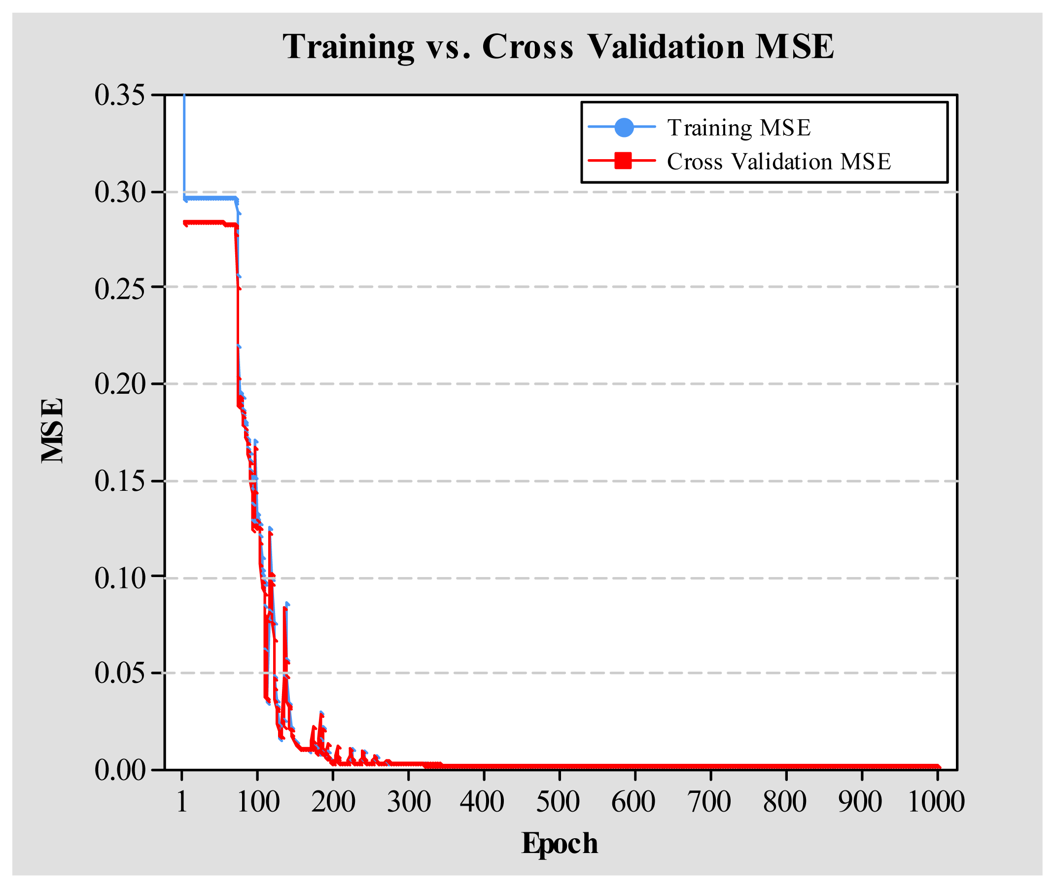
Figure 4 shows the mean squared error (MSE) of the network after each epoch of data. The epoch number is shown on the X-axis and the MSE is shown on the Y-axis. The MSE of the training set is shown in blue and the MSE of the cross-validation set is shown in red. The cross validation MSE tracks the training MSE closely after an approximate epoch of 75. A network that is trained well should have a constantly decreasing slope of the training MSE (typically an exponential decay). As long as the training set learning curve is decreasing, the network is still training. If the training set learning curve is increasing or bouncing up and down, the network is probably not training well (learning rates may need to be decreased) [16].
The specified data sets are training, cross validation and testing. Training data are the portion of the data used to actually train the network and are normally the largest portion of data. Cross validation data are used to intermittently validate the training. Periodically testing the network (no weight changes during cross validation) during training can help avoid overspecializing on the training data. Cross validation data are data set aside to test the network during training (the network parameters are not directly updated/trained with this data). It is used to stop the network training when the network starts to specialize too much on the training data. Testing data are used to further validate the results of a trained network. Although the network was not trained with the cross validation data, the training may have been stopped using it. Therefore, the cross validation data are not truly “out-of-sample”. The testing data are data set aside to test the network after it has been trained and is truly “out-of-sample”.
Cross-validation is a practical, reliable, well documented approach for testing the performance of forecasting models and is used for most machine learning techniques. Unfortunately, one can never eliminate the possibility of getting stuck in a local optimum. Here it was necessary in the developed neural network's training and testing to obtain the mean performance value across n trials. Additionally, cross-validation was used to make sure that the model was not over trained. Without cross-validation, neural networks tend to be easily overly trained, reproducing training set observations thereby rendering the model ineffective. A classical technique of gradually reducing the learning rate, then increasing it and then slowly drawing it down was employed. This approach was repeated several times. Raising the learning rate reduces the stability of the algorithm but gives the algorithm the ability to jump out of a local optimum.
Figure 5 is graphical representation of the developed NeuroSolutions supervised Multi-Layer Perceptron (MLP) network used in this research to forecast electrical demand. It consists of multiple layers of processing elements (PEs) connected in a feed forward fashion. The PEs in the developed network are the orange circular icons and are called axons. The connections between the PEs are the icons with horizontal and diagonal lines between the axons and are called synapses. Back propagation of errors is used to train the MLP. The smaller icons on top of the axons and synapses are called back propagation components and pass the error backwards from the end of the network to the beginning. The green axons on top of the back-propagation components are called momentum gradient search components and adjust the weights contained in the synapses and axons. The 2nd axon from the right is the output axon and generates the actual network outputs. The 1st axon on the left is called the input axon and it does nothing but accept the input from the file component. The two middle axons are the hidden layers. The red and orange dials at the upper left are the back-propagation controllers. They contain learning parameters like the learning mode (batch, online, etc.).
Each neural component encapsulates the functionality of a particular piece of the neural network. A working neural network simulation requires the interaction of many different components. As mentioned before, adaptive learning using gradient descent and focuses on using the error between the system output and the desired system output to train the system. The learning algorithm adapts the weights of the system based on the error until the system produces the desired output.
The goal of the developed network is for the system output to be the same as the desired output. This is accomplished by minimizing the mean squared error, and the method used is called error back-propagation. This is done through three main steps; first, the input data are propagated forward through the network to compute the system output. Next, the error is computed and propagated backward through the network. And lastly, the error is used to modify the weights.
In the proposed methodology approximately 2/3 of the 90-day recorded data on all inputs and output were used as training data. Approximately 1/3 of the 90 recorded data on all inputs and output were used for cross validation. And finally, two work weeks were used for testing the network performance.
4. Experimental Results
The performance of the proposed forecast method for predicting total building kW demand in a large government building is presented in this section. Ninety days of uninterrupted data, at a sample rate of 15 s, were captured at the large government building. Due to nature of the building's daily operations schedule, peak demand events were only observed occurring during the work week; specifically Monday through Friday. Since there was never a chance of a peak event occurring on a weekend day, it was only necessary to test the ANN for peak demand on working weekdays.
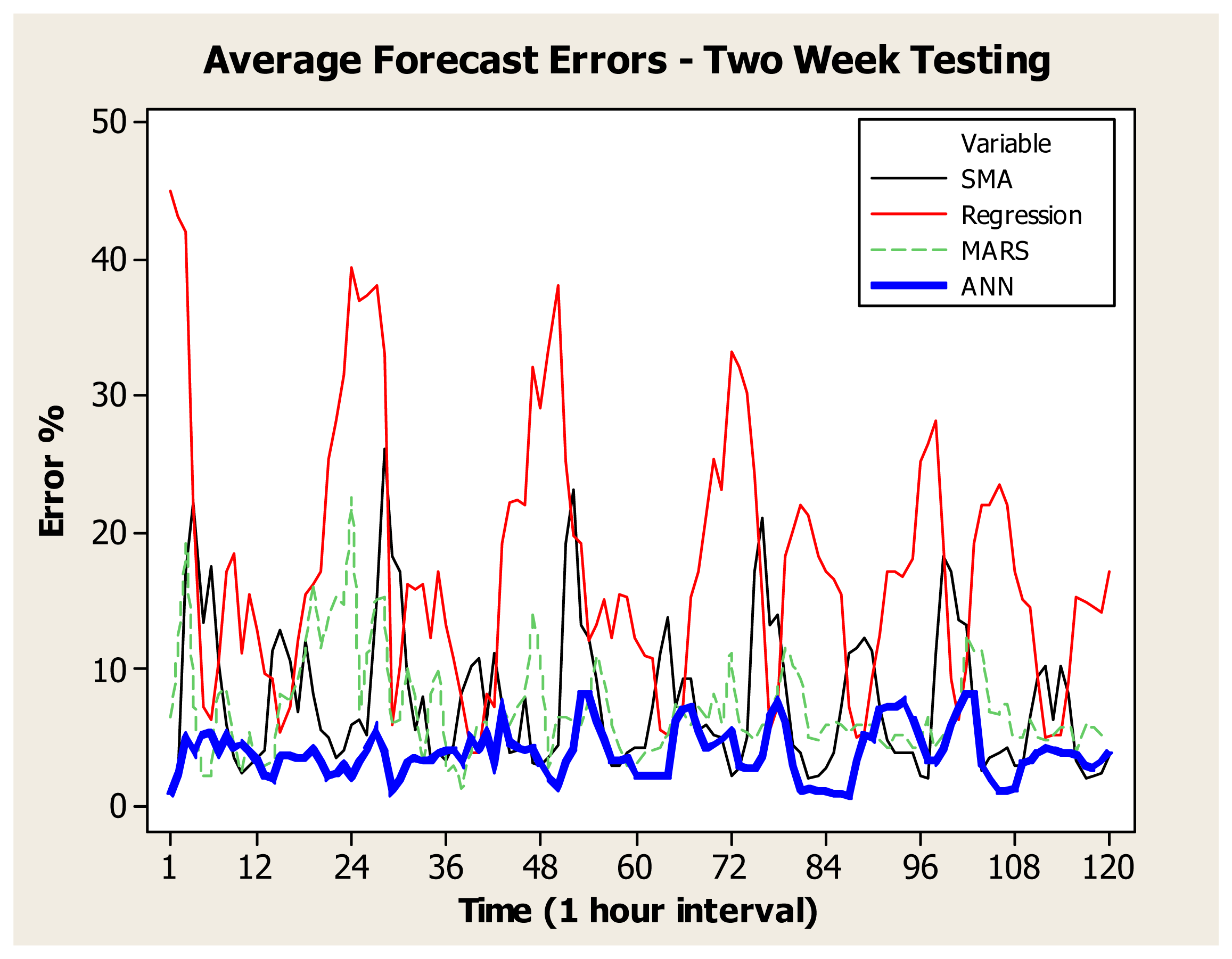
Using the testing data set, a sixty-minute forward forecast using the ANN model was tested for each workday day type in a given work week (Monday–Friday) for two weeks. In an effort to validate the neural network performance during unique periods of experienced demand of each workday day type, testing was conducted every hour (240 data points, 15 s sampling) beginning Monday 12:00 am through Friday 11:59 pm. Two weeks were tested and Table 2 depicts the average sixty-minute ANN forecasting errors realized for both work weeks. Also using the same test data, the ANN model's performance was compared against three other benchmark models: SMA, linear regression, and MARSplines. Table 2 also depicts the entire work week's sixty-minute forecasting errors for the SMA, linear regression, and MARSplines benchmark models for both weeks. The average of both testing work week's sixty-minute forecasting errors for all models are also plotted in Figure 6. Table 3 depicts twenty-four hour period MAPEs and AMEs for the ANN and benchmarking models during both testing weeks. For the developed ANN model, the MAPE and AME for all tested day types was 3.9% and 8.2% respectively. The benchmark models and their respective forecast errors are detailed next.
A SMA benchmark model was created for comparison. The moving average was limited to sixty minutes of past data to predict sixty minutes into the future. The average and maximum forecast error for all tested day types using a SMA was 7.7% and 26.2% respectively.
For another benchmark comparison model, linear regression using Minitab version 16.2.4 was applied to the original 90-day data set. The regression equation resulted as:
The regression equation was then applied to the same twenty-four hour data test periods with respective forecast errors depicted in Table 2. The average and maximum forecast error for all tested day types using linear regression was 17.3% and 45.1% respectively. Additionally, the residual regression plots for the 90-day data set demonstrated acceptable randomness of the data.
Also, for ANN model performance testing, Multivariate Adaptive Regression Splines (MARSplines) were implemented using StatSoft's STATISTICA version 12 and were applied to the original 90-day data set. MARSplines, developed by Friedman in 1991, were used here as a nonparametric regression procedure and do not assume any functional relationship between the dependent and independent variables. Rather, MARSplines relate the dependent and independent variables using a set of coefficients and basic functions derived directly from the regression data. MARSplines create regression equations for multiple unique regions within the input space. Furthermore, when the relationship between the predictors and the dependent variables is non-monotone and difficult to approximate with parametric models, MARSplines are capable of creating effective forecast models.
The STATISTICA MARSplines Regression equation resulted as:
The MARSplines equation was then applied to the same twenty data test periods with respective forecast errors depicted in Table 2. The average and maximum forecast error for all tested day types using MARSplines was 7.0% and 22.5%, respectively.
5. Conclusions
This paper proposes a real-time energy monitoring system prototype to forecast peak demand in a large government building in an effort to augment current ICS DR programs. The proposed methodology aims to predict total building power kW demand sixty minutes into the future, thereby giving building management ample time to temporarily curtail a portion of building power consumption in order to minimize experienced peak demand (kW) during a given billing cycle. To achieve this, the model collects detailed electrical consumption data in a large government building over a ninety-day time period which are then fed to an ANN for training, cross-validation, and finally prediction.
The approach in this paper used ANNs because of the extraordinary ability of ANNs to make sense of complicated or imprecise non-linear, non-stationary, and/or chaotic data which cannot be easily modeled. ANNs can extract patterns, detect complex trends, do not require a priori problem space assumptions, and do not require information regarding statistical distribution. ANNs also demonstrate adaptability to new situations through adaptive learning. ANNs produce unique representations of the information during its learning process, operate in real-time, and are capable of parallel computation. Furthermore, ANNs have inherent built-in fault tolerance as a result of redundant information coding.
The real-time energy monitoring system developed to capture the building's electrical consumption demonstrated high resolution capability of recording every main service entrance and HVAC circuit's (3-phase) power consumption in the building under study with a sample rate of 15 s. Operating within a customized LAN, Magnelab current transformer sensors, National Instruments DAQ devices, and National Instruments LabVIEW served as the backbone of the developed real-time energy monitoring system.
To examine and demonstrate the effectiveness of this research approach, experimental analysis was conducted on electrical consumption data recorded over a three-month period. Dynamic HVAC kW loads were able to offer accurate forecasting of total building demand. By also incorporating day type, time of day, exterior temperature, and humidity data into the developed ANN, the forecast error was minimized even further. Model performance was consistent throughout the test runs. Also, the developed ANN model was compared with alternate methods of prediction including SMA, linear regression and multivariate adaptive regression splines (MARSplines) and consistently performed better with an MAPE of 3.9% and AME of 8.2%. The SMA model performed well due to the static nature of the building's power consumption, but the MAPE was quite high at 26.2%. Performing similarly, the MARSplines approach had an MAPE of 7.0% and AME of 22.5%. Finally, linear regression had the highest MAPE of 17.3% and highest AME of 45.1%.
Given sixty-minute forecast ability with low error using the ANN approach, it is theoretically possible for building management to temporarily curtail a portion of the building load whenever approaching a predetermined peak in demand. Due to seasonality effects on the building's HVAC load, acceptable peak demand loads differ from month to month. It is thus necessary for building management to determine an acceptable peak demand load maximum for each billing cycle. The real-time energy monitoring system together with the sixty-minute ANN forecast signals an upcoming breach of the predetermined peak demand load maximum. Building curtailment policy sheds unnecessary loads during these events in order to control overall peak loading and prevent an unwanted peak demand occurrence. Depending on building management, curtailment is manual and/or automated. This ANN model would be particularly useful for efficient and cost-effective peak demand energy management of multiple government or corporate building complexes (i.e., municipalities, corporate campuses, hospitals, universities, etc.) already under or capable of operating under one centralized energy management or building management system. The proposed model is entirely scalable and can be implemented for multi-building peak demand control. Existing sub-meters at such sites would serve to provide pertinent real-time and historical data to the ANN model and control procedures. Overall reduced peak demand would have a noticeable and beneficial financial impact on such building systems. If implemented on a large scale across many building systems including city municipalities and other large energy end-users, there would be added benefit to the electric utility provider and environment through efficient and reduced power generation capacity. Such reduction and efficient usage of power generation would undoubtedly contribute to the energy sustainability of local municipalities and their communities.
Finally, the model developed in this paper was implemented and tested during one of two major local weather periods. The model proved effective during the particular weather period studied with similar performance expected during similar future weather periods. In order to measure the model's robustness during a dissimilar weather period, additional testing and data capture during the other weather period type is necessary.
Acknowledgments
This research has been partially funded by a grant from the local municipality for the University of Miami Department of Industrial Engineering as an extension of the American Recovery and Reinvestment Act which included federal funds (appropriated by the Obama Administration and the U.S. Congress in 2009) awarded to local municipalities and earmarked for green energy initiatives.
Conflicts of Interest
The authors declare no conflict of interest.
Nomenclature
| ANN | Artificial Neural Network |
| SMA | Simple Moving Average |
| MARSplines | Multivariate Adaptive Regression Splines |
| MAPE | Mean Absolute Percentage Error |
| AME | Absolute Maximum Error |
| kW | Kilowatt |
| kWh | Kilowatt Hour |
| DSM | Demand Side Management |
| DR | Demand Response |
| TOU | Time of Use |
| RTP | Real-Time Pricing |
| CPP | Critical-Peak Pricing |
| DLC | Direct Load Control |
| HVAC | Heating Ventilation and Air-Conditioning |
| ICS | Interruptible/Curtailable Service |
| DBB | Demand Bidding Buyback |
| EDR | Emergency Demand Response |
| CM | Capacity Market |
| ASM | Ancillary Services Market |
| HP | Horsepower |
| MCC1 | Motor Control Center 1 |
| MCC2 | Motor Control Center 2 |
| MSE1 | Main Service Entrance 1 |
| MSE2 | Main Service Entrance 2 |
| MSE3 | Main Service Entrance 3 |
| CT | Current Transducer |
| NI | National Instruments |
| cRIO | Compact Real-Time Input Output |
| VI | Virtual Instrument |
| RMS | Root Mean Square |
| Hz | Hertz |
| MLP | Multilayer Perceptron |
| PE | Processing Element |
| MSE | Mean Square Error |
References
- Rahman, S. Smart grid expectations [in my view]. IEEE Power Energy Mag. 2009, 7, 88–84. [Google Scholar]
- Faria, P.; Vale, Z. Demand response in electrical energy supply: An optimal real time pricing approach. Energy 2011, 36, 5374–5384. [Google Scholar]
- Vale, Z.; Pinto, T.; Praça, I.; Morais, H. MASCEM: Electricity markets simulation with strategic agents. IEEE Intell. Syst. 2011, 26, 9–17. [Google Scholar]
- Electricity Advisory Committee. Keeping the Lights on in a New World; U.S. Department of Energy: Washington, DC, USA, 2009; p. 50. [Google Scholar]
- Albadi, M.H.; El-Saadany, E.F. A summary of demand response in electricity markets. Electr. Power Syst. Res. 2008, 78, 1989–1996. [Google Scholar]
- International Energy Agency. The Power to Choose: Demand Response in Liberalised Electricity Markets; OECD Publishing: Paris, France, 2003. [Google Scholar]
- Woo, C.K.; Greening, L.A. Guest editors' introduction. Energy 2010, 35, 1515–1517. [Google Scholar]
- U.S. Department of Energy. Benefits of Demand Response in Electricity Markets and Recommendations for Achieving Them; A Report to the United States Congress; U.S. Department of Energy: Washington, DC, USA, 2006. [Google Scholar]
- Avci, M.; Erkoc, M.; Rahmani, A.; Asfour, S. Model predictive HVAC load control in buildings using real-time electricity pricing. Energy Build. 2013, 60, 199–209. [Google Scholar]
- Hippert, H.S.; Pedreira, C.E.; Souza, R.C. Neural networks for short-term load forecasting: A review and evaluation. IEEE Trans. Power Syst. 2001, 16, 44–55. [Google Scholar]
- Czernichow, T.; Piras, A.; Imhof, K.; Caire, P.; Jaccard, Y.; Dorizzi, B.; Germond, A. Short term electrical load forecasting with artificial neural networks. Eng. Intell. Syst. Electr. Eng. Commun. 1996, 4, 85–100. [Google Scholar]
- Bakirtzis, A.G.; Theocharis, J.B.; Kiartzis, S.J.; Satsios, K.J. Short-term load forecasting using fuzzy neural networks. IEEE Trans. Power Syst. 1995, 10, 1518–1524. [Google Scholar]
- Mori, H.; Kobayashi, H. Optimal fuzzy inference for short-term load forecasting. IEEE Trans. Power Syst. 1996, 11, 390–396. [Google Scholar]
- Papadakis, S.E.; Theocharis, J.B.; Kiartzis, S.J.; Bakirtzis, A.G. A novel approach to short-term load forecasting using fuzzy neural networks. IEEE Trans. Power Syst. 1998, 13, 480–492. [Google Scholar]
- Khotanzad, A.; Afkhami-Rohani, R.; Maratukulam, D. ANNSTLF—Artificial neural network short-term load forecaster—Generation three. IEEE Trans. Power Syst. 1998, 13, 1413–1422. [Google Scholar]
- Principe, J.C.; Euliano, N.R.; Lefebvre, W.C. Neural and Adaptive Systems: Fundamentals through Simulations with CD-ROM; John Wiley & Sons, Inc.: Hoboken, NJ, USA, 1999. [Google Scholar]
- Kosko, B. Neural Networks and Fuzzy Systems; Prentice-Hall: Upper Saddle River, NJ, USA, 1992. [Google Scholar]
- Escrivá-Escrivá, G.; Álvarez-Bel, C.; Roldán-Blay, C.; Alcázar-Ortega, M. New artificial neural network prediction method for electrical consumption forecasting based on building end-uses. Energy Build. 2011, 43, 3112–3119. [Google Scholar]
- Youssef, H.A.; Al-Makky, M.Y.; Eltoukhy, M.A. Evaluation of a proposed neural network predictive model for grind-hardening. Alex. Eng. J. 2003, 42, 411–417. [Google Scholar]

| Floor(s) | Usage |
|---|---|
| Basement | Parking, Electrical Service Entrance, Chillers' Mechanicals |
| 1 | Main Entrance, Building Management, Parking Violations, Cafeteria |
| 2–4 | Courtrooms |
| 5–7 | Judges Chambers |
| 8–9 | Administrative |
| 10 | HVAC Mechanicals |
| Weekday | Model | 12:00 AM | 1:00 AM | 2:00 AM | 3:00 AM | 4:00 AM | 5:00 AM | 6:00 AM | 7:00 AM | 8:00 AM | 9:00 AM | 10:00 AM | 11:00 AM | 12:00 PM | 1:00 PM | 2:00 PM | 3:00 PM | 4:00 PM | 5:00 PM | 6:00 PM | 7:00 PM | 8:00 PM | 9:00 PM | 10:00 PM | 11:00 PM |
|---|---|---|---|---|---|---|---|---|---|---|---|---|---|---|---|---|---|---|---|---|---|---|---|---|---|
| Monday | SMA | 1.5 | 1.9 | 17.2 | 22.3 | 13.4 | 17.5 | 10.4 | 5.9 | 3.5 | 2.3 | 2.9 | 3.5 | 4.1 | 11.3 | 12.9 | 10.5 | 6.9 | 12.1 | 8.2 | 5.5 | 4.9 | 3.5 | 4.1 | 5.9 |
| Regression | 45.1 | 43.2 | 42.1 | 22.1 | 7.2 | 6.2 | 10.5 | 17.2 | 18.4 | 11.2 | 15.4 | 12.9 | 9.7 | 9.2 | 5.4 | 7.2 | 12.1 | 15.4 | 16.2 | 17.2 | 25.4 | 28.2 | 31.5 | 39.5 | |
| MARSplines | 6.5 | 12.2 | 19.2 | 7.2 | 2.1 | 2.1 | 8.2 | 8.5 | 4.2 | 2.5 | 5.4 | 2.5 | 2.9 | 3.1 | 8.2 | 7.5 | 9.2 | 11.2 | 16.3 | 11.5 | 14.1 | 15.2 | 14.8 | 22.5 | |
| ANN | 0.8 | 2.2 | 4.9 | 3.9 | 5.2 | 5.3 | 3.9 | 5.1 | 4.2 | 4.5 | 3.9 | 3.3 | 2.1 | 1.9 | 3.6 | 3.7 | 3.5 | 3.5 | 4.1 | 3.2 | 2.1 | 2.3 | 2.9 | 2.1 | |
| Tuesday | SMA | 6.2 | 5.2 | 15.2 | 26.2 | 18.2 | 17.2 | 9.1 | 5.5 | 7.9 | 3.5 | 3.9 | 3.2 | 4.5 | 8.2 | 10.2 | 10.8 | 6.2 | 11.2 | 7.5 | 3.9 | 4.1 | 7.9 | 3.1 | 2.9 |
| Regression | 37.1 | 37.3 | 38.2 | 33.1 | 5.9 | 10.2 | 16.2 | 15.9 | 16.3 | 12.2 | 17.2 | 13.2 | 10.8 | 7.9 | 3.9 | 3.8 | 8.2 | 7.2 | 19.2 | 22.2 | 22.4 | 22.1 | 32.1 | 29.2 | |
| MARSplines | 6.9 | 11.2 | 15.1 | 15.2 | 5.9 | 6.2 | 10.2 | 7.9 | 2.9 | 8.2 | 10.2 | 2.5 | 2.9 | 1.3 | 3.9 | 5.9 | 6.1 | 2.2 | 7.2 | 5.9 | 7.2 | 8.0 | 14.2 | 10.2 | |
| ANN | 3.2 | 4.1 | 5.5 | 3.9 | 1.1 | 1.9 | 3.2 | 3.5 | 3.2 | 3.3 | 3.9 | 4.1 | 4.0 | 3.2 | 5.0 | 4.2 | 5.2 | 3.2 | 6.8 | 4.6 | 4.2 | 4.1 | 4.2 | 3.0 | |
| Wednesday | SMA | 3.5 | 4.5 | 19.2 | 23.1 | 13.2 | 12.2 | 9.2 | 5.2 | 2.9 | 2.9 | 3.9 | 4.2 | 4.3 | 7.2 | 11.2 | 13.8 | 7.2 | 9.2 | 9.3 | 5.5 | 5.9 | 5.2 | 4.9 | 2.2 |
| Regression | 33.2 | 38.2 | 25.2 | 19.8 | 19.2 | 12.0 | 13.2 | 15.1 | 12.3 | 15.4 | 15.2 | 12.2 | 10.9 | 10.7 | 5.5 | 5.2 | 5.3 | 7.5 | 15.2 | 17.2 | 21.2 | 25.4 | 23.1 | 33.2 | |
| MARSplines | 2.8 | 6.5 | 6.5 | 6.3 | 5.9 | 7.8 | 11.0 | 9.0 | 5.9 | 4.2 | 2.9 | 2.8 | 3.8 | 4.1 | 4.2 | 5.2 | 7.5 | 6.9 | 5.9 | 7.2 | 6.2 | 8.2 | 6.0 | 11.2 | |
| ANN | 2.0 | 1.4 | 3.2 | 4.2 | 8.2 | 8.1 | 6.2 | 4.9 | 3.3 | 3.3 | 3.5 | 2.2 | 2.1 | 2.1 | 2.1 | 2.2 | 6.2 | 7.1 | 7.2 | 5.4 | 4.2 | 4.5 | 4.9 | 5.4 | |
| Thursday | SMA | 2.7 | 4.9 | 17.2 | 21.0 | 13.2 | 13.9 | 9.1 | 4.4 | 3.8 | 1.9 | 2.2 | 2.8 | 3.8 | 7.2 | 11.2 | 11.6 | 12.2 | 11.4 | 7.2 | 4.8 | 3.9 | 3.8 | 3.8 | 2.2 |
| Regression | 32.1 | 30.2 | 24.3 | 15.2 | 5.5 | 7.2 | 18.2 | 20.1 | 22.1 | 21.2 | 18.2 | 17.2 | 16.5 | 15.4 | 7.2 | 4.9 | 5.3 | 9.2 | 12.5 | 17.2 | 17.1 | 16.8 | 18.1 | 25.2 | |
| MARSplines | 5.9 | 5.3 | 4.9 | 5.9 | 6.2 | 8.2 | 11.5 | 10.2 | 9.2 | 4.9 | 4.7 | 5.9 | 6.1 | 5.9 | 5.3 | 5.9 | 5.8 | 5.9 | 4.9 | 4.2 | 5.1 | 5.2 | 4.2 | 4.2 | |
| ANN | 2.9 | 2.7 | 2.7 | 3.5 | 6.5 | 7.6 | 6.1 | 2.9 | 1.1 | 1.2 | 1.0 | 1.0 | 0.9 | 0.8 | 0.7 | 3.3 | 5.1 | 4.9 | 7.1 | 7.2 | 7.2 | 7.6 | 6.4 | 4.9 | |
| Friday | SMA | 1.9 | 11.1 | 18.2 | 17.2 | 13.5 | 13.2 | 6.9 | 2.5 | 3.5 | 3.9 | 4.2 | 3.0 | 3.0 | 6.5 | 9.5 | 10.2 | 6.2 | 10.2 | 8.2 | 3.2 | 2.0 | 2.1 | 2.4 | 3.7 |
| Regression | 26.6 | 28.2 | 19.2 | 9.2 | 6.2 | 10.2 | 19.2 | 22.1 | 22.1 | 23.5 | 22.1 | 17.2 | 15.1 | 14.5 | 9.2 | 5.0 | 5.1 | 5.2 | 9.1 | 15.2 | 14.9 | 14.5 | 14.2 | 17.2 | |
| MARSplines | 6.4 | 4.2 | 5.2 | 6.1 | 7.1 | 12.5 | 11.2 | 11.3 | 6.9 | 6.7 | 7.4 | 4.9 | 4.9 | 6.2 | 4.9 | 4.7 | 5.2 | 5.8 | 5.8 | 3.9 | 5.9 | 5.7 | 5.2 | 4.9 | |
| ANN | 3.3 | 3.2 | 4.1 | 5.9 | 7.1 | 8.2 | 8.2 | 2.9 | 1.9 | 1.1 | 1.1 | 1.2 | 3.1 | 3.2 | 3.9 | 4.2 | 4.1 | 3.9 | 3.8 | 3.7 | 2.9 | 2.8 | 3.2 | 3.9 | |
| Weekday | Performance | SMA | Regression | MARSplines | ANN |
|---|---|---|---|---|---|
| Monday | Average | 8.0 | 19.5 | 9.0 | 3.4 |
| Max | 22.3 | 45.1 | 22.5 | 5.3 | |
| Tuesday | Average | 8.4 | 18.4 | 7.4 | 3.9 |
| Max | 26.2 | 38.2 | 15.2 | 6.8 | |
| Wednesday | Average | 7.9 | 17.1 | 6.2 | 4.3 |
| Max | 23.1 | 38.2 | 11.2 | 8.2 | |
| Thursday | Average | 7.5 | 16.5 | 6.1 | 4.0 |
| Max | 21.0 | 32.1 | 11.5 | 7.6 | |
| Friday | Average | 6.9 | 15.2 | 6.4 | 3.8 |
| Max | 18.2 | 28.2 | 12.5 | 8.2 | |
| Week | Week Average | 7.7 | 17.3 | 7.0 | 3.9 |
| Week Max | 26.2 | 45.1 | 22.5 | 8.2 | |


© 2014 by the authors; licensee MDPI, Basel, Switzerland. This article is an open access article distributed under the terms and conditions of the Creative Commons Attribution license ( http://creativecommons.org/licenses/by/3.0/).
Share and Cite
Grant, J.; Eltoukhy, M.; Asfour, S. Short-Term Electrical Peak Demand Forecasting in a Large Government Building Using Artificial Neural Networks. Energies 2014, 7, 1935-1953. https://doi.org/10.3390/en7041935
Grant J, Eltoukhy M, Asfour S. Short-Term Electrical Peak Demand Forecasting in a Large Government Building Using Artificial Neural Networks. Energies. 2014; 7(4):1935-1953. https://doi.org/10.3390/en7041935
Chicago/Turabian StyleGrant, Jason, Moataz Eltoukhy, and Shihab Asfour. 2014. "Short-Term Electrical Peak Demand Forecasting in a Large Government Building Using Artificial Neural Networks" Energies 7, no. 4: 1935-1953. https://doi.org/10.3390/en7041935
APA StyleGrant, J., Eltoukhy, M., & Asfour, S. (2014). Short-Term Electrical Peak Demand Forecasting in a Large Government Building Using Artificial Neural Networks. Energies, 7(4), 1935-1953. https://doi.org/10.3390/en7041935