Abstract
The Lagrange multiplier-based method is an effective network parameter error identification method. However, two full matrices with high-dimensions are involved in the calculation procedure; these create huge computational burdens for large-scale power systems. To solve this problem, a fast solution is proposed in this paper, where special treatment techniques for full matrices are used to dramatically improve the calculation efficiency. A practical parameter error identification program has been developed and used in many electric power control centers. In this paper, the results for test systems and on-site applications are given, which show that the proposed approach is very efficient.1. Introduction
Identifying network parameter errors is important because they can seriously diminish the accuracy of various kinds of power system analyses. State estimation (SE) is very helpful for parameter error identification (PEI) [1], since the measurement residuals may directly indicate the parameter errors. Most existing PEI methods are based on SE results.
There are two types of traditional PEI methods. The first type is based on sensitivity analysis [2–8]. These methods use sensitivity factors between measurements and parameters, along with the measurement residuals to find the most suspicious network parameters. An important advantage of these methods is that they are directly based on the SE results; therefore, current SE software can be used without any modification. However, the results of sensitivity factor-based PEI methods may be affected by artificial threshold values and random measurement errors. An offline application has been recently reported in [9]. The second type of PEI methods is based on augmented state estimation (ASE) [10–13]. ASE methods augment the parameter errors to the state variables and obtain their estimated values through SE calculation. The suspicious parameter set is limited by the numerical condition problem and should be obtained before calculation. This type of method is more appropriate for parameter estimation (PE) rather than PEI.
The recently proposed Lagrange multiplier (LM)-based method [14–16] is an effective PEI approach, but two high-dimension full matrices are involved during its calculation procedure. This represents a very heavy computational burden and requires huge memory. Furthermore, it is well known that network parameter error identifications should use multiple measurement scans to increase accuracy; the iterative usage of the LM-based PEI method requires a faster calculation speed, even for off-line applications.
The main contribution of this paper is the development of a fast approach for the Lagrange Multiplier (LM)-based PEI model. Specifically, the development concerns a treatment technique for full matrices. Based on the proposed approach, an efficient PEI program has been implemented, which has been used in several power system control centers. Extensive numerical tests on test systems and practical systems have been done to verify the performance of the developed PEI program.
2. Lagrange Multiplier-Based PEI
The LM-based network PEI procedure is based on the weighted least square (WLS) estimator. The procedure was proposed in [14]. The Lagrange Multiplier vector λ for equality constraints on network parameter errors can be calculated from:
To normalize the Lagrange Multiplier vector λ, its covariance matrix Λ = cov(λ) should be computed first:
The normalized LM λN can be calculated as:
In the LM-based network PEI method, the normalized LM vector λN can then be used as the index for identifying suspicious network parameters. To identify errors in network parameters (along with those of measurements), the LM-based PEI procedure proceeds as follows:
Perform SE, and obtain the normalized measurement residual vector rN.
Calculate λN using Equations (1)–(4).
If the max| λN, rN| < α, where α is a threshold value that can be taken as 3.0, proceed to step 4.
Otherwise:
If the max |λN| ≤ max |rN|, the measurement corresponding to max |rN| should be considered as erroneous and be removed from the active measurement set. Return to step 1.
If the max |λN| > max |rN|, the parameter corresponding to max |λN| should be considered as erroneous; modify the corresponding parameter by PE and return to step 1.
Output the PEI and SE results.
Calculating the normalized LM vector λN is critical for the LM-based network PEI method; such calculations involve determining Λ. However, two full matrices, S and Σ, are involved in the calculation procedure for the covariance matrix Λ. The dimensions of S and Σ are m and 2n−1; respectively. For large scale practical power systems, their dimensions may exceed 10,000 or more; this necessitates a prohibitive amount of calculation time and memory storage.
3. Solution
This section will provide an efficient method for calculating Λ(i,i). To simplify the presentation, the discussions in this section are based on the decoupled SE method. Similarly, the uncoupled form can be derived. In Hx, if Hx(i,j) ≠ 0, measurement i is said to be relative to state variable j. In Hp, if Hp(i,c) ≠ 0, then measurement i is said to be relative to parameter c. All the measurements relative to parameter c form the relative measurement set of parameter c (expressed by φc). The symmetric production of φc is called the relative dual measurement set for parameter c, and is expressed as ψc. For an arbitrary set φc = {a b d e}, its symmetric production ψc is defined as:
If one assumes H̃ = WHp, then Equation (2) can be expressed as:
The c-th diagonal elements Λ(c,c) can be calculated by:
Since H̃ is a sparse matrix, only the following elements in the full matrix S have to be calculated to determine Λ(c,c):
Therefore, the subscripted set of the necessary elements in S is exactly the relative dual measurement set ψc for parameter c. Assume that parameter c belongs to branch l; according to the measurement functions, the relative measurement set φc is formed by the branch power and the terminal node injection power measurements of branch l. The relative dual measurement set ψc can also be derived easily according to φc.
The necessary subscript set ψΣ for calculating all of the diagonal elements in Λ is:
Therefore, only a few elements in the full matrix S have to be calculated. This significantly reduces the calculation burden. However, the calculation of S in Equation (2) still involves a full matrix Σ. According to Equation (2), S(k,q) is calculated by:
For a specified branch l, its relative measurements, k and q, include both its branch power and its power injection measurements (of l's terminal nodes). For branch power measurements, the relative nodes will only include the terminal nodes of l. For power injection measurements, the relative nodes will include their neighbor nodes. In summary, the node indices, i, j, for the elements in Σ necessary to calculate Λ(c,c) can be obtained from the symmetric production of the node set formed by the terminal node of branch l and their neighbor nodes (if the terminal node has injection measurement).
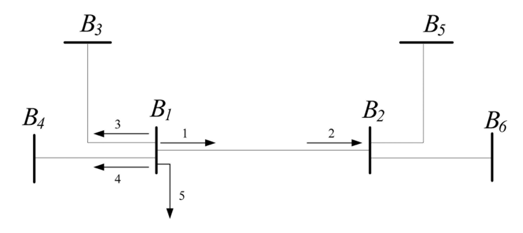
Taking the simple branch shown in Figure 1 as an example, the arrows numbered 1 through 5 stand for measurements, and B1-B6 represent the six nodes. The necessary element set in matrix S is the symmetric production of the measurement set {1, 2, 5}, which can be expressed as {(1, 2), (1, 5), (2, 5)}. The necessary element set in matrix Σ is the symmetric production of nodes B1, B2 (terminal nodes), and B3, B4 (neighbor nodes of B1, since B1 has injection measurements). The elements with rows or columns corresponding to nodes B5 and B6 are unnecessary to calculate, since no injection measurements exist in node B2. The necessary element set in matrix Σ is {(B1, B2), (B1, B3), (B1, B4), (B2, B3), (B2, B4), (B3, B4)}.
In summary, the necessary elements in S, as well as in Σ, can be conveniently selected according to the node-branch relationship, and the calculation burden of the diagonal elements of matrix Λ can be greatly reduced.
After the necessary elements in Σ and S are known, we can use Equations (7) and (10) to calculate these elements. Furthermore, it can be concluded that if the branches with small measurement residuals can be pre-filtered, only a part of the branch parameters will participate in the PEI calculation, and the necessary elements of S and Σ can be decreased even more significantly, thereby increasing the calculation efficiency even more.
4. Numerical Tests
4.1. Measurement Pre-Processing
Gross errors in measurements can deteriorate the results of any PEI method. An SE program with a bad data identification function will distinguish all measurements into two groups: good data (G) and bad data (B). Notably, some measurements are surely erroneous in the set B, while the other measurements may be correct, but are infected by parameter errors. Distinguishing between erroneous measurements and measurements infected by parameter errors is very important. The former will deteriorate the PEI results and should be excluded in PEI calculations while the latter is very important evidence of parameter errors.
To maintain calculation efficiency, a simplified method of consistency checking is used. A simple branch is shown in Figure 1 as an example.
For a branch power measurement in set B (such as measurement 1 in Figure 1): if |z1 − z2| < c max (|z1|,|z2|), it is justified that measurement 1 is correct but infected by parameter errors. Otherwise, it is justified that measurement 1 is erroneous. Here, c is a constant that equals 0.1 in this paper.
For an injection measurement in set B (such as measurement 5 in Figure 1): if |z1 + z3 + z4 + z5| < c max (|z1|,|z3|,|z4|,|z5|), it is justified that measurement 5 is correct but infected by parameter errors. Otherwise, it is justified that measurement 5 is erroneous.
This method is based on a physical concept: when measurement errors occur simultaneously with high relative and consistent values, it is more reasonable that they originate from parameter errors (rather than from bad measurements). Then, a simplified PEI procedure can be obtained:
SE with bad data identification function. All measurements will be divided into the groups G and B.
Distinguish between erroneous measurements and measurements infected by parameter errors
Pre-filter the branches with small measurement residuals that will not take part in the PEI. In this paper, the branches are excluded from the PEI when the largest residual is smaller than 0.01 p.u.
Calculate the LM using normal measurements and measurements infected by parameter errors.
Calculate the diagonal elements in Λ based on the method proposed in Section 3.
Calculate the normalized LM.
This simplified PEI procedure no longer needs iterative SE, PEI or PE, and is thus very efficient. The PEI can be carried out based on the SE results directly, and the existing SE codes can be kept unchanged. A PEI program has been developed based on this simplified procedure and the efficient calculation method concerning the diagonal elements in the covariance matrix. This program is very efficient. Its performances on test systems and on-site test results are introduced as follows.
4.2. 9-Node System
Figure 2 shows the 9-node system in which the PEI procedure is illustrated. The SE is carried out based on commercial decoupled SE software and no modification has been made to the existing code. A single measurement scan is used in this example.
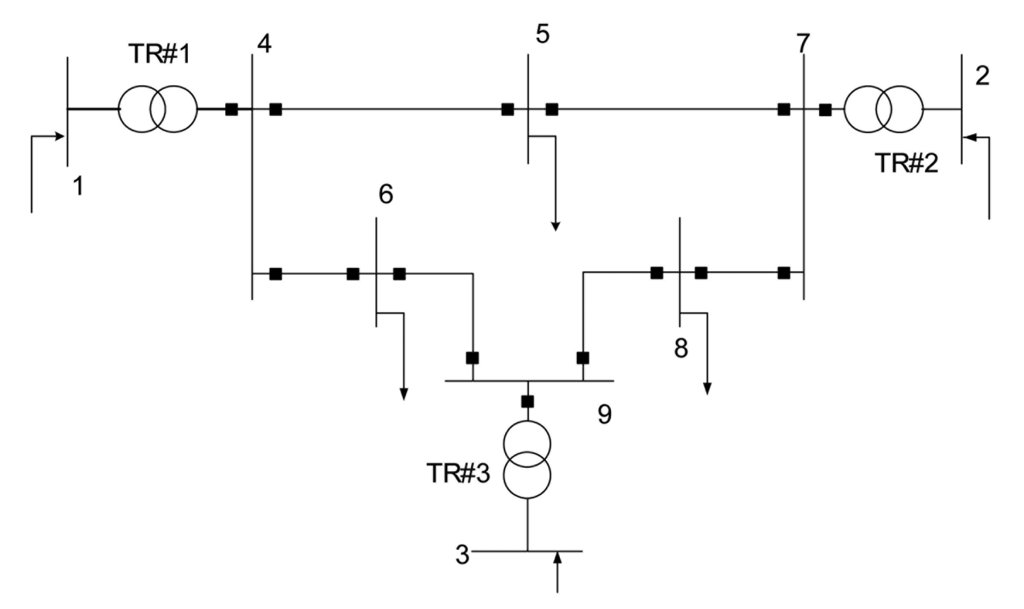
White noise, based on the real-load flow distribution of the 9-node system, is added to generate the measurement values. The standard deviations of the errors are taken as 0.01 for the power and 0.001 for the voltage measurements, respectively. The reactance of branch 9-8 has been changed manually from 0.1008 p.u. to 0.2016 p.u. as a parameter error, and the active power measurement of branch 4-6 has been changed manually from −30.57 MW to −60.57 MW to create a gross error. The PEI can be carried out step by step as described in subsection 4.1:
Perform SE: the suspicious measurements identified by bad data identification function are listed in Table 1, and the gross errors are in bold.
 Table 1. Suspicious measurements in a 9-node system.
From Table 1, it can be concluded that the first two measurements are infected by parameter errors, as their measurement values are consistent (24.16 MW & −24.10 MW). In contrast, the measurement P4-6 is an erroneous measurement, since its measurement value significantly mismatches with the measurement P6-4.
Pre-filter the branch with small measurement residuals. In this example, branches 9-8, 9-6, and 4-6 should take part in the PEI calculation. In fact, as the measurement and parameter errors are manually set, it can be concluded that the branch 8-9 has erroneous parameters; the branch 4-6 has no erroneous parameters but gross error measurement; and the branch 9-6 is infected by erroneous parameters and measurements.
LM values are listed in the 3rd column of Table 2.
Table 2. Detail results of the PEI in a 9-node system.The necessary elements in matrix S are drawn in Equation (12), where the measurement index M1−4 is a simplified expression of four measurements including P1-4, Q1-4, P4-1, and Q4-1, and M1 is a simplified expression of P1 and Q1.
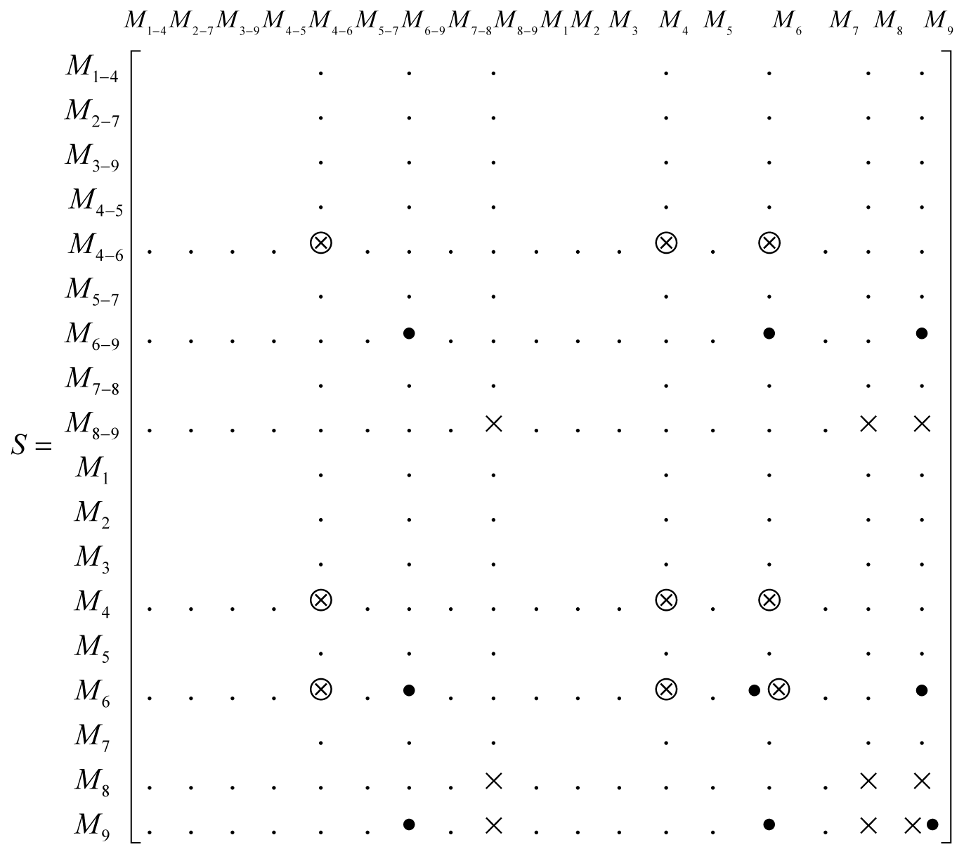
The necessary elements in the calculation of diagonal elements in matrix Λ, which correspond to the parameters of branches 9-8, 9-6, and 4-6, are highlighted by signals “×”, “•” and “⊗”, respectively. The signal “.” is used to show the position of the necessary elements more clearly and has no physical meaning. Taking branch 9-8 as an example, its relative measurements include M8−9 (branch power measurements), and M8 and M9 (injection power measurements for terminal nodes); the necessary measurements in S are the diagonal and cross elements of these three groups of measurements (expressed by ×). Similarly, the necessary elements in Σ are shown in Equation (13):
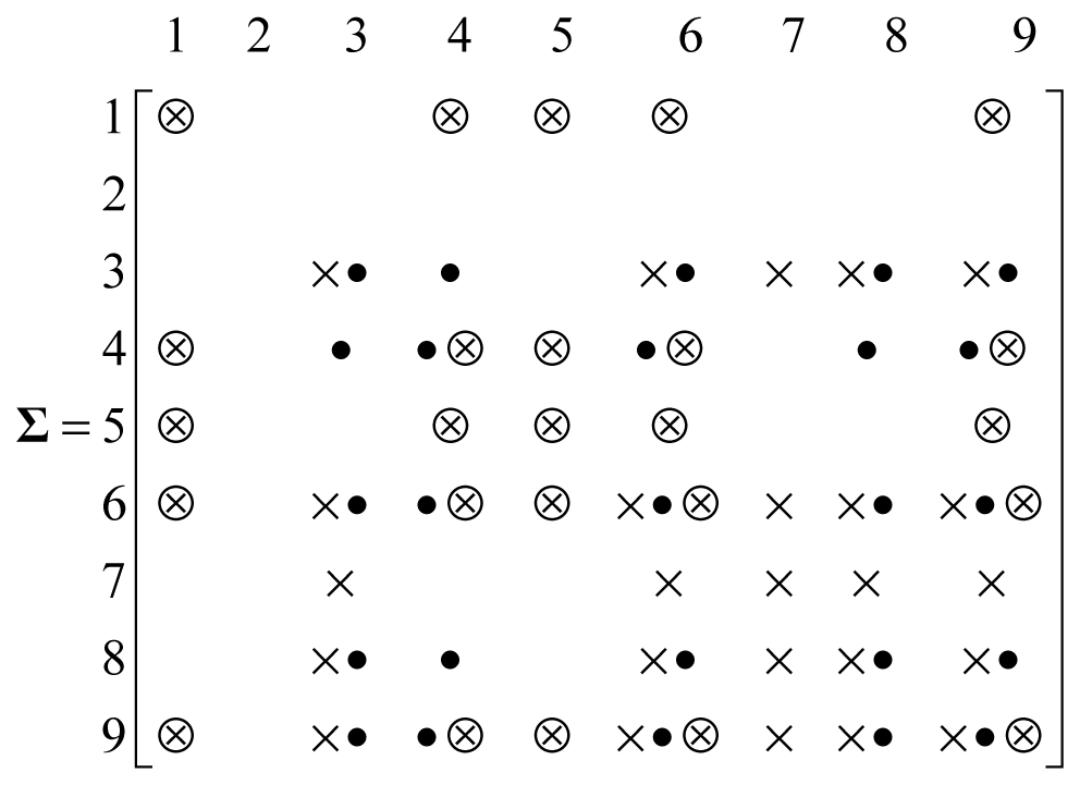
Taking branch 9-8 as an example, the terminal nodes 9 and 8 both have injection measurements (node 9 has zero injection measurements), and the necessary elements in Σ include the terminal nodes (8, 9) and their neighbor nodes (3, 6, 7). The diagonal and cross elements corresponding to these five nodes are necessary and highlighted by “×”:
The normalized LM values are listed in the last column of Table 2. The reactance of branch 9-8 has the largest normalized LM, and has been correctly identified as a parameter error.
Average necessary element rates in S: S is a 1098 × 1098 full matrix in this test. The necessary element rates are calculated in Figure 3; their values are all less than 0.1%.
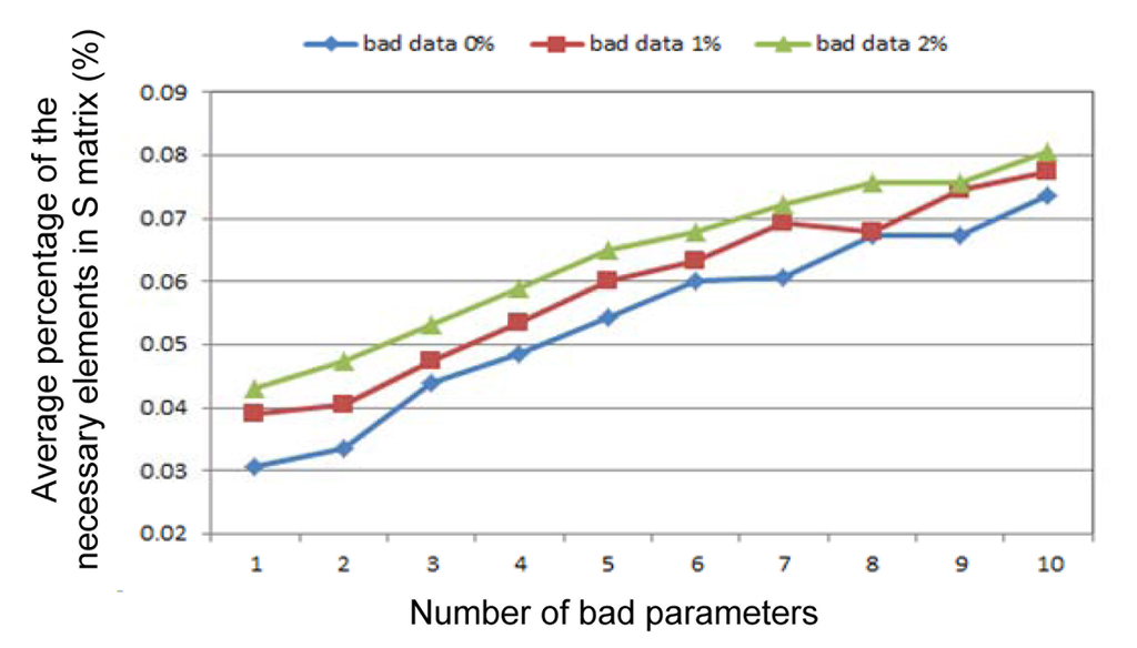 Figure 3. Average necessary element rates in the S matrix.
Average necessary element rates in Σ: since decoupled SE software is used, Σ is a 118 × 118 full matrix in both the P-sub and Q-sub iterations. The necessary element rates are calculated in Figure 4; their values are all less than 6.5%.
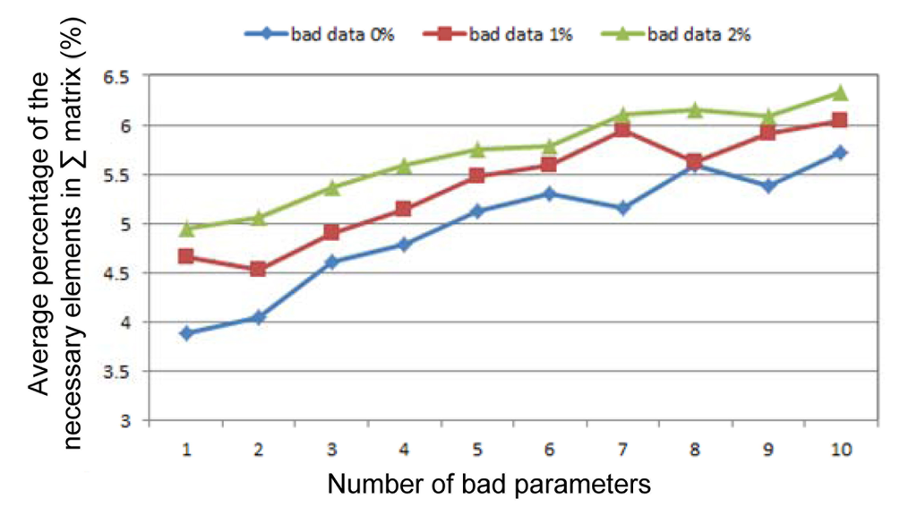 Figure 4. Average necessary element rates in the Σ matrix.
- Zarco, P.; Exposito, A.G. Power system parameter estimation: A survey. IEEE Trans. Power Syst. 2000, 15, 216–222. [Google Scholar]
- Fletcher, D.; Stadlin, W. Transformer tap position estimation. IEEE Trans. Power Appar. Syst. 1983, 102, 3680–3686. [Google Scholar]
- Liu, W.; Wu, F.; Lun, S. Estimation of parameter errors from measurement residuals in state estimation. IEEE Trans. Power Syst. 1992, 7, 81–89. [Google Scholar]
- Mukherjee, B.; Fuerst, G.; Hanson, S.; Monroe, C. Transformer tap estimation—Field experience. IEEE Trans. Power Appar. Syst. 1984, 103, 1454–1458. [Google Scholar]
- Quintana, V.; van Cutsem, T. Real-time processing of transformer tap positions. Can. Electr. Eng. J. 1987, 12, 171–180. [Google Scholar]
- Smith, R. Transformer tap estimation at Florida power corporation. IEEE Trans. Power Appar. Syst. 1985, 104, 3442–3445. [Google Scholar]
- Van Cutsem, T.; Quintana, V. Network parameter estimation using online data with application to transformer tap position estimation. IEE Gener. Trans. Distrib. 1988, 135, 31–40. [Google Scholar]
- Do Coutto Filho, M.B.; Stacchini de Souza, J.C.; Meza, E.B.M. Off-line validation of power network branch parameters. IET Gener. Trans. Distrib. 2008, 2, 892–905. [Google Scholar]
- Castillo, M.; London, J.; Bretas, N.G. Offline detection, identification, and correction of branch parameter errors based on several measurement scans. IEEE Trans. Power Syst. 2011, 26, 870–877. [Google Scholar]
- Alsac, O.; Vempati, N.; Stott, B.; Monticelli, A. Generalized state estimation. IEEE Trans. Power Syst. 1998, 13, 1069–1075. [Google Scholar]
- Slutsker, I.; Clements, K. Real time recursive parameter estimation in energy management systems. IEEE Trans. Power Syst. 1996, 11, 1393–1399. [Google Scholar]
- Handschin, E.; Kliokys, E. Transformer tap position estimation and bad data detection using dynamic signal modeling. IEEE Trans. Power Syst. 1995, 10, 810–817. [Google Scholar]
- Teixeira, P.A.; Brammer, S.R.; Rutz, W.L.; Merritt, W.C.; Salmonsen, J.L. State estimation of voltage and phase-shift transformer tap settings. IEEE Trans. Power Syst. 1992, 7, 1386–1393. [Google Scholar]
- Zhu, J.; Abur, A. Identification of network parameter errors. IEEE Trans. Power Syst. 2006, 21, 586–592. [Google Scholar]
- Zhu, J.; Abur, A. Improvement in network parameter error identification via synchronized phasors. IEEE Trans. Power Syst. 2010, 24, 244–250. [Google Scholar]
- Zhang, L.; Abur, A. Improved network parameter error identification using multiple measurements scans. Proceedings of the 17th Power System Computation Conference, Stockholm, Sweden, 22–26 August 2011.
From the above example of the 9-node system, it can be concluded that only a few elements are necessary to the calculation. The simplified PEI procedure is very efficient, and is based directly on the SE results.
4.3. 118-Node System
To comprehensively evaluate the efficiency of the proposed method, extensive numerical tests have been done on the IEEE 118-node system. The measurements construction is same as the 9-node system tests'. To test the performance of the PEI program with different rates of gross errors, three classes of tests with 0, 1, and 2% bad measurement rates are produced, where the standard error of bad measurements is of 100 times that of normal measurements. In each class, 10 groups of tests with 1, 2, …, 10 parameter errors are produced. The error parameter fell between 2–10 times the true value 50% of the time, and between 0.1–0.5 times the true value the rest of the time. A total of 900 tests (with 30 samples each) have been selected. To evaluate the effectiveness of the proposed Λ matrix calculation method, the following two indices were counted:
From Figures 3 and 4, it can be concluded that the proposed calculation method for the diagonal elements of Λ is very effective. Less than 6.5% of the elements of Σ and 0.1% of the elements of S need to be calculated. Therefore, the proposed method can significantly increase the efficiency of the PEI and can make practical the LM-based PEI for real-world applications.
4.4. Practical Application
In practical application, multiple measurement scans are used to increase the accuracy [16]. Employing LM for PEI and ASE for PE, this program has been used in several electric power control centers in China. As an example, the results of a provincial power system with 500 buses in Central China are shown. To this end, 96 continuous scans with 15-minutes intervals are realized and the results are presented in Table 3. The reactance of the “Luoanjia line” has the largest normalized (LM). The PE results also indicate that this parameter is erroneous (the estimated value of 1.3928 p.u. is far from its initial 3.2600 p.u.). The relative measurement residuals before and after parameter modification are listed in Table 4. Before parameter modification, the relative measurements have significant residuals (4th column), which indicates the existence of parameter errors. However, after modifying X of the Luoanjia line (from the initial value 3.2600 p.u. to the estimated value 1.3928 p.u.), these measurement residuals decreased significantly (6th column), leading to the conclusion that these parameter identifications and estimation system results are reasonable.
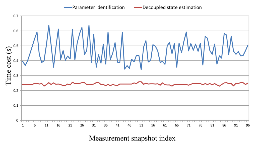
Figure 5 shows the computation times of PEI and decoupled SE. In this practical system, the computation time of the PEI procedure is less than 0.7 seconds for each measurement scan; this is only about twice SE's computational time. The developed LM-based PEI program is very efficient and is absolutely acceptable for on-site application.
5. Conclusions
It is very important to maintain network parameter accuracy with high efficiency in power systems. In this paper, an efficient solution for the Lagrange multiplier-based parameter error identification method is proposed. A parameter error identification program based on the Lagrange multiplier has been developed and put into real practice at several electric power control centers in China. The results of test systems and practical systems demonstrate the effectiveness and efficiency of the proposed solution.
Acknowledgments
This work is supported by National High Technology Research Program (2011AA05A118), National Science Foundation of China (51177080), and National Science Fund for Distinguished Young Scholars (51025725)
Conflicts of Interest
The authors declare no conflict of interest.
References
© 2014 by the authors; licensee MDPI, Basel, Switzerland. This article is an open access article distributed under the terms and conditions of the Creative Commons Attribution license ( http://creativecommons.org/licenses/by/3.0/).
Acknowledgments
This work is supported by National High Technology Research Program (2011AA05A118), National Science Foundation of China (51177080), and National Science Fund for Distinguished Young Scholars (51025725)
Conflicts of Interest
The authors declare no conflict of interest.
References
- Zarco, P.; Exposito, A.G. Power system parameter estimation: A survey. IEEE Trans. Power Syst. 2000, 15, 216–222. [Google Scholar]
- Fletcher, D.; Stadlin, W. Transformer tap position estimation. IEEE Trans. Power Appar. Syst. 1983, 102, 3680–3686. [Google Scholar]
- Liu, W.; Wu, F.; Lun, S. Estimation of parameter errors from measurement residuals in state estimation. IEEE Trans. Power Syst. 1992, 7, 81–89. [Google Scholar]
- Mukherjee, B.; Fuerst, G.; Hanson, S.; Monroe, C. Transformer tap estimation—Field experience. IEEE Trans. Power Appar. Syst. 1984, 103, 1454–1458. [Google Scholar]
- Quintana, V.; van Cutsem, T. Real-time processing of transformer tap positions. Can. Electr. Eng. J. 1987, 12, 171–180. [Google Scholar]
- Smith, R. Transformer tap estimation at Florida power corporation. IEEE Trans. Power Appar. Syst. 1985, 104, 3442–3445. [Google Scholar]
- Van Cutsem, T.; Quintana, V. Network parameter estimation using online data with application to transformer tap position estimation. IEE Gener. Trans. Distrib. 1988, 135, 31–40. [Google Scholar]
- Do Coutto Filho, M.B.; Stacchini de Souza, J.C.; Meza, E.B.M. Off-line validation of power network branch parameters. IET Gener. Trans. Distrib. 2008, 2, 892–905. [Google Scholar]
- Castillo, M.; London, J.; Bretas, N.G. Offline detection, identification, and correction of branch parameter errors based on several measurement scans. IEEE Trans. Power Syst. 2011, 26, 870–877. [Google Scholar]
- Alsac, O.; Vempati, N.; Stott, B.; Monticelli, A. Generalized state estimation. IEEE Trans. Power Syst. 1998, 13, 1069–1075. [Google Scholar]
- Slutsker, I.; Clements, K. Real time recursive parameter estimation in energy management systems. IEEE Trans. Power Syst. 1996, 11, 1393–1399. [Google Scholar]
- Handschin, E.; Kliokys, E. Transformer tap position estimation and bad data detection using dynamic signal modeling. IEEE Trans. Power Syst. 1995, 10, 810–817. [Google Scholar]
- Teixeira, P.A.; Brammer, S.R.; Rutz, W.L.; Merritt, W.C.; Salmonsen, J.L. State estimation of voltage and phase-shift transformer tap settings. IEEE Trans. Power Syst. 1992, 7, 1386–1393. [Google Scholar]
- Zhu, J.; Abur, A. Identification of network parameter errors. IEEE Trans. Power Syst. 2006, 21, 586–592. [Google Scholar]
- Zhu, J.; Abur, A. Improvement in network parameter error identification via synchronized phasors. IEEE Trans. Power Syst. 2010, 24, 244–250. [Google Scholar]
- Zhang, L.; Abur, A. Improved network parameter error identification using multiple measurements scans. Proceedings of the 17th Power System Computation Conference, Stockholm, Sweden, 22–26 August 2011.
© 2014 by the authors; licensee MDPI, Basel, Switzerland. This article is an open access article distributed under the terms and conditions of the Creative Commons Attribution license ( http://creativecommons.org/licenses/by/3.0/).