1. Introduction
Ultracapacitors (UCs), known by different names such as supercapacitors, electrochemical double-layer capacitors, double-layer capacitors or electrochemical capacitors, have the potential to meet the high pulse power capability of the energy-storage systems for automotive applications [
1]. UCs offer higher power density and longer shelf and cycle life than batteries. The primary disadvantage of UCs is their lower energy density as compared to that of batteries [
2]. In the high pulse power operations for automotive applications, a large amount of heat is produced inside a UC cell [
3]. Because the lifetime and performance of a UC depend strongly on temperature [
4,
5], it is important to be able to accurately predict the electrical and thermal behaviors of a UC for its efficient and reliable system integration from an application perspective. Modeling of the electrical and thermal behaviors of a UC can serve a valuable role when optimizing the design of future cells and the thermal management system for automotive applications [
6].
There have been many previous studies on modeling UCs, and the reviews of UC models are available [
6,
7,
8]. Spyker and Nelms [
9] suggested the classical equivalent circuit composed of a capacitor, an equivalent parallel resistance, and an equivalent series resistance to model the electrical behavior of a UC. In slow discharge applications on the order of a few seconds, the classical equivalent circuit for a UC can adequately describe capacitor performance. Zubieta and Bonert [
10] proposed an electrical model consisting of three resistor-capacitor (RC) branches to achieve a better fit to the collected data on the electrical behavior of a UC than the classical equivalent circuit. De Levie [
11] developed a theory on the capacitance in each pore of porous electrodes being modeled as an RC transmission line. Previous thermal models predicted the thermal behavior of a UC by solving the transient heat conduction equation in one- [
12], two- [
13,
14], or three-dimensional space [
15,
16,
17]. Most of those thermal models [
13,
15,
16,
17] neglected the reversible heat generation in a UC cell. Schiffer
et al. [
18] showed that the heat generation in a UC cell consists of an irreversible Joule heat and a reversible heat caused by a change of entropy based on the analysis of the thermal measurement data obtained for a UC. They derived a mathematical expression of Joule heat from the electric equivalent circuit of the UC. They provided a mathematical representation of the reversible heat generation by interpreting the entropy as a measure of disorder: ions in the electrolyte are ordered near the interface between the electrode and electrolyte during charge and they are spreading themselves again during discharge. Dandeville
et al. [
19] developed a calorimetric technique for determing time-dependent heat profiles of electrochemical capacitors. The profiles were extracted from the temperature change of the capacitor under cycling. Measuring results suggested that the irreversible heat was caused by the Joule loss through the porous structure and the reversible heat by the ion adsorption on the carbon surface. Guillemet
et al. [
20] presented multi-level reduced-order thermal modeling based on both numerical and analytical approaches. Bohlen
et al. [
5] analyzed different types of electrochemical capacitors in accelerated ageing tests by impedance spectroscopy. They developed an ageing model based on the characteristic changes of the impedance parameters. Al Sakka
et al. [
6] developed a thermal model based on thermal-electric analogy and determined the supercapacitor temperature. They studied the heat management of supercapacitor modules for vehicle applications by using their model. Gualous
et al. [
14] developed a thermal model to study the supercapacitor temperature distribution in steady and transient states. They placed a thermocouple inside the supercapacitor to validate their model. D’Entremont and Pilon [
12] developed a physical modeling of the coupled electrodiffusion, heat generation, and thermal transport occurring in electric double layer capacitors. They derived the governing energy equation from first principles and coupled with the modified Poisson-Nernst-Planck model for transient electrodiffusion. They recently presented a first-order thermal model of electric double layer capacitors based on the lumped-capacitance approximation [
21]. Their model can be regarded as a zero-dimensional thermal model in comparison with the one- [
12], two- [
13,
14], or three-dimensional models [
15,
16,
17] introduced in the above.
In this work, modeling is performed to study the electrical and thermal behaviors of a 2.7 V/650 F UC cell from LS Mtron Ltd. (Anyang, Korea). A three-branch RC circuit model is employed to calculate the electrical behavior of the UC. To predict the thermal behavior of the UC, both of the irreversible and reversible heat generations in the UC cell are considered. The validation of the modeling approach is provided through the comparison of the modeling results with the experimental measurements.
2. Mathematical Model
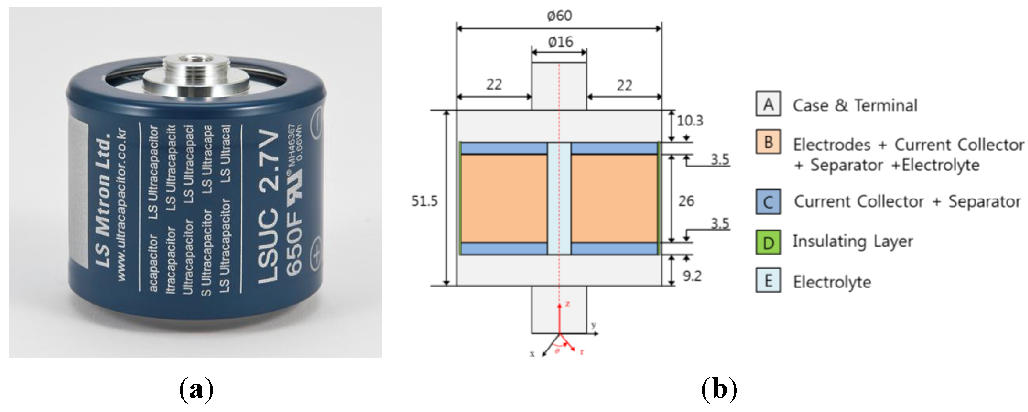
A cylindrical 2.7 V/650 F UC cell from LS Mtron Ltd. is modeled in this work.
Figure 1a shows the external appearance of the UC cell. A schematic diagram of the construction of the cell is shown in
Figure 1b. It is divided into five major regions: (A) the case and terminal made of aluminum; (B) the spiral winding of activated carbon electrodes coated on the current collectors made of aluminum and the porous separators made of polypropylene immersed in the electrolyte whose main constituent is propylene carbonate; (C) the current collector edges which are not coated with electrode materials electrically connected to terminals and the separators; (D) the insulating layer made of polypropylene between the regions of (B) and (C) and the region of (A); and (E) the void filled with electrolyte along the axis of cylinder.
Figure 1.
(a) Photograph of the ultracapacitor (UC) cell; and (b) schematic diagram of the construction of the cell.
Figure 1.
(a) Photograph of the ultracapacitor (UC) cell; and (b) schematic diagram of the construction of the cell.
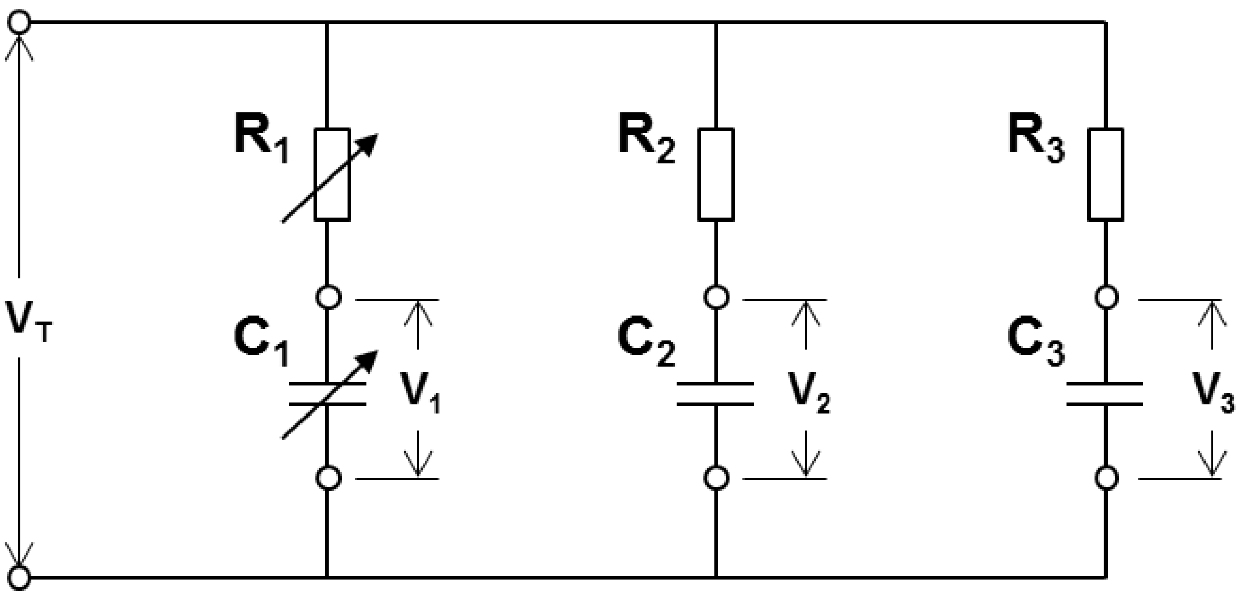
The three RC parallel branch model proposed in this work to simulate the electrical behavior of the UC cell is shown in
Figure 2. The three RC branch model is primarily based on the work of Zubieta and Bonert [
10]. In order to ensure the simplicity and accuracy of the model, three RC branch model was chosen, although a large number of RC branches may be favorable to capture the nonlinear electrical behaviors of UC. Zubieta and Bonert [
10] called the three branches the immediate, delayed, and long-term branches, respectively. Each of the three branches has a distinct time constant differing from the others. The immediate branch with the elements
R1 and
C1 dominates the immediate behavior in order of a few seconds. The delayed branch with the elements
R2 and
C2 dominates the immediate behavior in the range of minutes. The long-term branch with the elements
R3 and
C3 dominates the behavior for times longer than ten minutes. To set up a practical engineering model in the present work, the nonlinear capacitance effect is included only in one RC element. Instead of adding an additional voltage-dependent capacitor branch in parallel with immediate branch capacitor as Zubieta and Bonert [
10] did, we make
R1 and
C1 current-dependent. Because the voltage across each branch is equal to the terminal voltage of the UC shown in
Figure 2, the following equation can be written for each branch:
where
VT is the terminal voltage (V) of the UC;
i1,
i2,
i3 are the currents (A) flowing through the first, second, and third branches of
Figure 2, respectively;
R1,
R2,
R3 are the resistances (Ω) of the first, second, and third branches of
Figure 2, respectively; and
V1,
V2,
V3 are the capacitor voltages (V) of the first, second, and third branches of
Figure 2, respectively. The currents flowing through first, second, and third branches of
Figure 2 are given as the multiplication of the branch capacitance and the time derivative of branch capacitor voltage as follows:
where
C1,
C2,
C3 are the capacitances (F) of the first, second, and third branches of
Figure 2, respectively; and
t is the time (s). Alternatively, these currents can be obtained from Equation (1) as follows:
Figure 2.
Three resistor-capacitor (RC) parallel branch model.
Figure 2.
Three resistor-capacitor (RC) parallel branch model.
Because the terminal current of the UC is equal to the summation of the three branch currents, the following equation for the terminal current can be written as:
where
I is the terminal current (A) of the UC. By substituting Equations (2)–(4) and Equations (5)–(7) into Equation (8), the following equations for the branch capacitor and terminal voltages can be derived as follows:
where
RT is the equivalent resistance (Ω) of three parallel branches. The parameters used to calculate the electrical behavior of the UC are given in
Table 1. As mentioned previously, we make
C1 and
R1 dependent on the terminal current,
I, while we make
C2,
C3,
R2, and
R3 constants. The parameter values are chosen to provide the best fit of the modeling results to the experimental data.
Table 1.
Parameters used to calculate the electrical behavior of the UC.
Table 1.
Parameters used to calculate the electrical behavior of the UC.
| Parameter (unit) | 50 A cycling | 100 A cycling | 150 A cycling | 200 A cycling |
|---|
| C1 (F) | 4.22 × 10² | 3.80 × 10² | 3.70 × 10² | 3.30 × 10² |
| C2 (F) | 2.07 × 10² | 2.07 × 10² | 2.07 × 10² | 2.07 × 10² |
| C3 (F) | 1.40 × 101 | 1.40 × 101 | 1.40 × 101 | 1.40 × 101 |
| R1 (Ω) | 6.49 × 10⁻⁴ | 4.00 × 10⁻⁴ | 3.60 × 10⁻⁴ | 2.80 × 10⁻⁴ |
| R2 (Ω) | 1.00 × 10⁻² | 1.00 × 10⁻² | 1.00 × 10⁻² | 1.00 × 10⁻² |
| R3 (Ω) | 2.31 × 10⁻² | 2.31 × 10⁻² | 2.31 × 10⁻² | 2.31 × 10⁻² |
To simplify the mathematical analysis of the thermal modeling, it is assumed that heat is generated only in the electrode region during the charge and discharge of the UC and the heat generation rate is uniform throughout the electrode region (A) [
15]. The heat generation in a UC cell is the summation of an irreversible Joule heat and a reversible heat caused by a change of entropy [
18]. The irreversible Joule heat generation rate (W),
QJ, is calculated by using the terminal current,
I, of the UC and the equivalent resistance,
RT, of three RC parallel branches as:
The reversible heat generation rate (W),
QR, is calculated by using the terminal current,
I, of the UC and the absolute temperature (K),
Tabs, as:
where α is a fitting parameter (V·K
−1). Although Schiffer
et al. [
18] derived an explicit expression for
QR, it contains parameters which are difficult to evaluate for porous electrodes and treating α as a fitting parameter is a more practical approach. The value of α used to calculate reversible heat generation in this work is 0.0008 (V·K
−1). The parameter value of α is chosen to provide the best fit of the modeling results to the experimental data. Once the heat generation rate in the electrode region (A) is determined as described in the above, the three-dimensional temperature distributions in the UC cell are obtained by solving the transient three-dimensional equation of heat conduction [
22] as follows:
where ρ is the density (kg·m
−3);
Cp is the specific heat capacity at constant pressure (J·kg
−1·°C
−1);
T is the temperature (°C);
kr,
kθ, and
kz are the effective thermal conductivities along the
r, θ, and
z directions (
Figure 1b) (W·m
−1·°C
−1), respectively; and
q is the heat generation rate per unit volume (W·m
−3). The effective density and specific heat capacity of the various compartments of the cell can be estimated based on the mass fractions of the components of each cell compartment [
15]. The effective thermal conductivities of the various compartments of the cell can be estimated based on the equivalent networks of parallel and series thermal resistances of the cell components [
15]. The parameters used to calculate the thermal behavior of the UC based on the three-dimensional model are given in
Table 2.
Table 2.
Thermal properties of UC cell compartments used for three-dimensional modeling.
Table 2.
Thermal properties of UC cell compartments used for three-dimensional modeling.
| Component | ρ (kg·m−3) | Cp (J·kg−1·°C−1) | k (W·m−1·°C−1) | Reference |
|---|
| Case | 2700 | 898.15 | 237 | [23] |
| Activated carbon | 700 | 700 | 5 | [24] |
| Current collector | 2700 | 898.15 | 237 | [23] |
| Electrolyte | 779.3 | 2230 | 0.19 | [23] |
| Separator | 930 | 1340 | 0.11 | [23] |
| Insulating layer | 930 | 1340 | 0.11 | [23] |
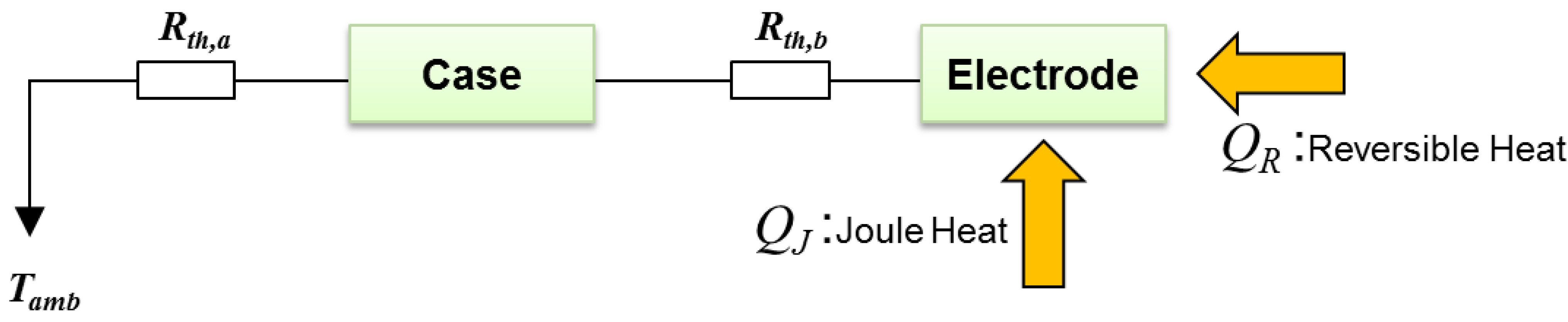
Because the three-dimensional thermal model requires significant computing resources, it is desirable to set up a simple thermal model which captures accurately the salient features of the thermal behavior of UC for automotive applications. The computational time of the simple model has to stay below the real-time requirements to obtain a real-time optimal controller of the thermal management system of the UC. To this end, we propose a zero-dimensional thermal model as in the following. The UC cell is divided the two regions of the electrode region (A) which generates heat during charge and discharge and the case and terminal region (B) which does not generate heat due to charge and discharge and we treat each region as a single point. The heat transfer between the electrode region (A) and the case and terminal region (B) occurs through thermal conduction and the heat is transferred from the case and terminal region (B) to the ambient air through thermal convection as shown schematically in
Figure 3.
Figure 3.
Schematic diagram of a zero-dimensional thermal model for the UC.
Figure 3.
Schematic diagram of a zero-dimensional thermal model for the UC.
The thermal resistance due to thermal conduction between the electrode region (A) and the case and terminal region (B),
Rth,a, is written as:
where Δ
x,
k, and
A are the effective conduction length (m), effective thermal conductivity (W·m
−1·°C
−1), and effective cross-sectional area (m
2), respectively, between the electrode and case [
22]. The thermal resistance due to the convective heat transfer between the case and terminal region (B) and ambient air,
Rth,b, is:
where
h and
A are the convective heat transfer coefficient (W·m
−2·°C
−1) and contact area (m
2), respectively, between the case and terminal region (B) and ambient air [
22]. Then, the temperatures of the electrode region (A) and the case and terminal region (B) are obtained by solving the following energy balance equations [
22]:
where
me and
mc are the lumped masses (kg) based on the mass fractions of the components of the electrode region (A) and the case and terminal region (B), respectively;
Ce and
Cc are the lumped specific heat capacities (J·kg
−1·°C
−1) based on the mass fractions of the components of the electrode region (A) and the case and terminal region (B), respectively; and
Te,
Tc, and
Tamb are the temperatures of the electrode region (A), the case and terminal region (B), and the ambient air (°C), respectively. The parameters used to calculate the thermal behavior of the UC based on the zero-dimensional thermal model are given in
Table 3.
Table 3.
Parameters used to calculate the thermal behavior of the UC based on the zero-dimensional thermal modeling.
Table 3.
Parameters used to calculate the thermal behavior of the UC based on the zero-dimensional thermal modeling.
| Thermal property | Unit | Value |
|---|
| me | kg | 9.675 × 10⁻² |
| mc | kg | 1.182 × 10⁻¹ |
| Ce | J·kg−1·°C−1 | 1204 |
| Cc | J·kg−1·°C−1 | 892 |
| Rth,a | °C·W−1 | 3.7 |
| Rth,b | °C·W−1 | 0.3 |
3. Results and Discussion
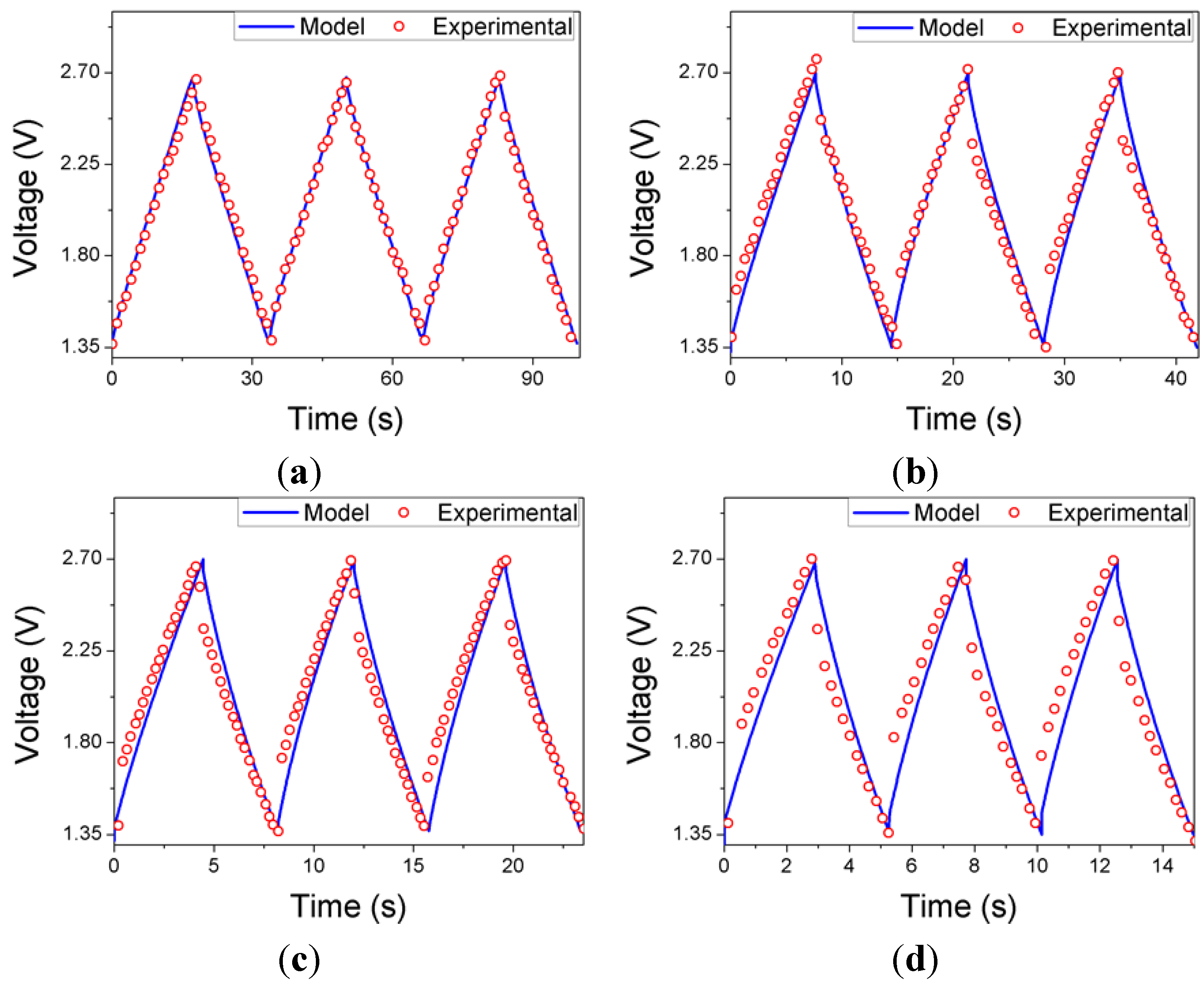
To test the validity of the modeling approach adopted in this work, the performance of 2.7 V/650 F UC cell from LS Mtron Ltd. was measured during cycling. A battery cycle life test system LCN 2-200-12 (Bitrode, St. Louis, MO, USA) was used to charge and discharge the UC cell. The system provides voltages and currents of up to 18 V and 200 A, respectively, with an accuracy of ±0.1% of the full scale. The measurement system for the electrical behavior of the UC cell was connected to the computer for the control of charge and discharge cycle and the data acquisition. The test-procedure and logging data such as time, current, voltage, power, temperature, and ampere-hour are programmable with VisuaLCN Lab Client Software (Bitrode, St. Louis, MO, USA) on the Windows environment. The UC cell was placed in a constant temperature and humidity chamber TH-G-300 (Jeio Tech, Daejon, Korea) during the charge and discharge cycles. The constant temperature and humidity chamber is controlled by a microprocessor with an accuracy of ±0.3 °C and ±1.5% relative humidity, respectively. The UC was subject to the constant-current charge and discharge current cycles between the half-rated voltage (1.35 V) and the rated voltage (2.7 V). The charge/discharge current values examined were 50, 100, 150, and 200 A. The solutions to Equations (1)–(3) were obtained by using “ode23” solver of MATLAB. The modeling results for the variations of the UC cell voltages as a function of time for different charge/discharge currents are compared with the experimental data in
Figure 4. The modeling results shown in
Figure 4 are in good agreement with the experimental measurements.
The three-dimensional temperature distributions were calculated as a function of time at various charge/discharge currents by using the computational fluid dynamics software ANSYS Fluent, which employs the finite volume method. The finite volume mesh used for calculation has 657,533 cells and 114,586 nodes.
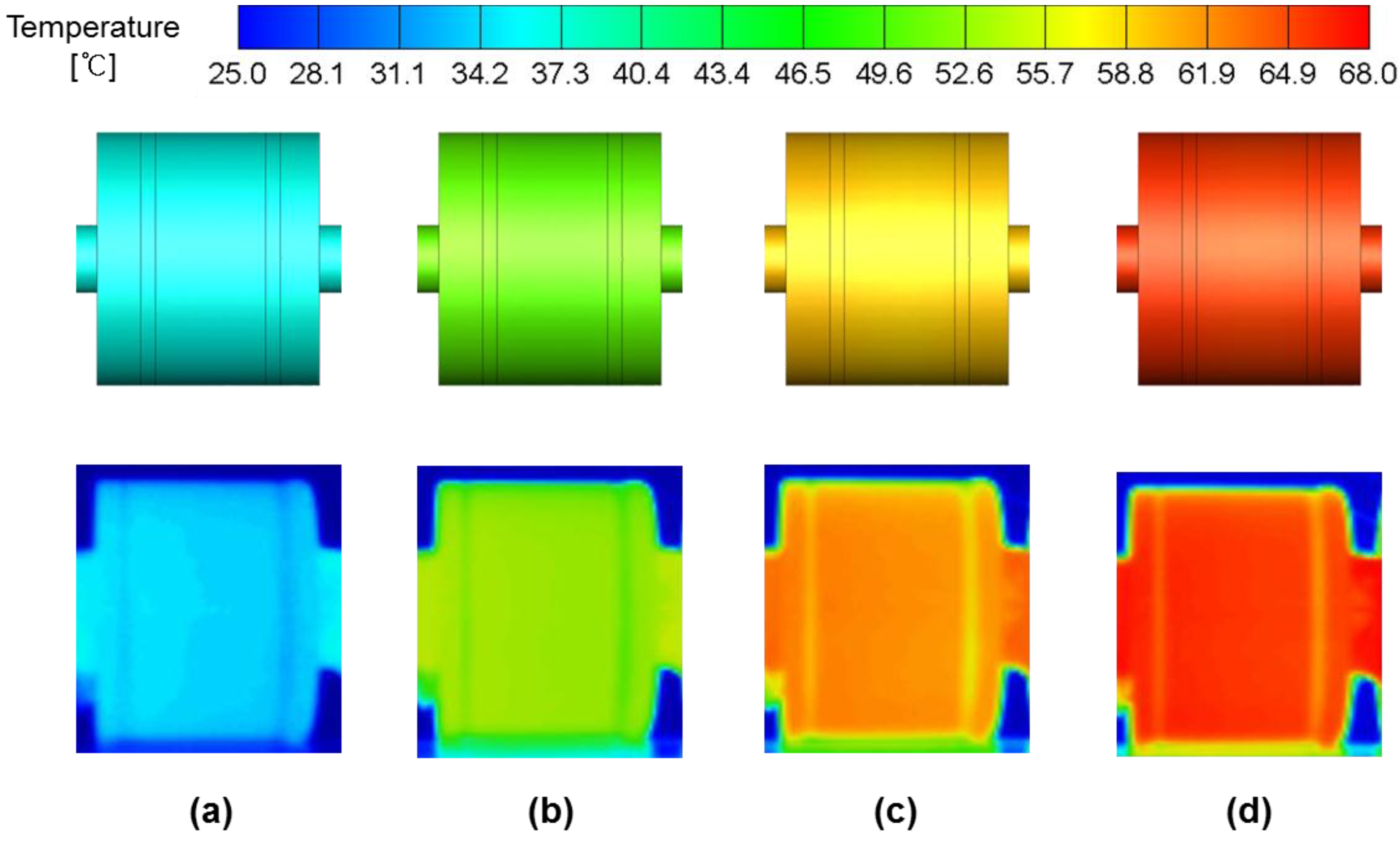
Figure 5 shows the temperature distributions based on the experimental infrared (IR) image and the modeling at cycling times of 300, 900, 1800, and 3600 s, respectively, for the charge/discharge current of 200 A. The overall temperature distributions obtained from the experiment and the modeling in
Figure 5 are in good agreement with each other.
Figure 4.
Comparison between the modeling results and experimental data for the variations of the UC cell voltages as a function of time at various charge/discharge currents of: (a) 50; (b) 100; (c) 150; and (d) 200 A.
Figure 4.
Comparison between the modeling results and experimental data for the variations of the UC cell voltages as a function of time at various charge/discharge currents of: (a) 50; (b) 100; (c) 150; and (d) 200 A.
Figure 5.
Temperature distributions based on the modeling (upper) and the experimental infrared (IR) image (lower) for the UC at cycling times of: (a) 300; (b) 900; (c) 1800; and (d) 3600 s for the charge/discharge current of 200 A.
Figure 5.
Temperature distributions based on the modeling (upper) and the experimental infrared (IR) image (lower) for the UC at cycling times of: (a) 300; (b) 900; (c) 1800; and (d) 3600 s for the charge/discharge current of 200 A.
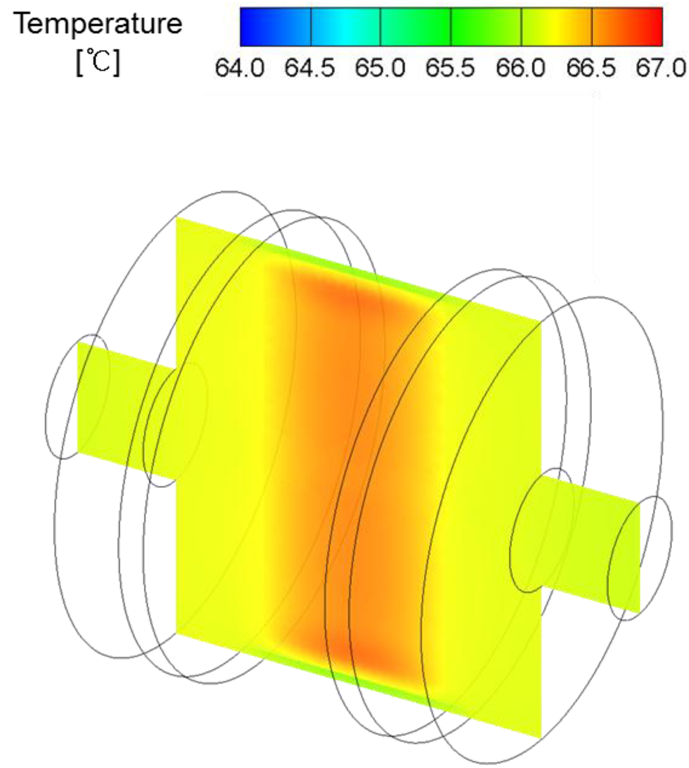
In
Figure 6, the temperature distribution inside the UC cell obtained from the modeling is shown at cycling time of 3600 s for the charge/discharge current of 200 A.
Figure 6 shows that the UC cell has roughly two distinct regions of relatively uniform temperature distribution. The temperatures of the electrode region (A) and the case and terminal region (B) have the values of 66.4 ± 0.5 °C and 65.1 ± 0.8 °C, respectively. The average temperature of the electrode region (A) is about 1.3 °C higher than that of the case and terminal region (B). The uniformity of the temperature distribution of the electrode region (A) is slightly higher than that of the case and terminal region (B), because the deviations of the minimum and maximum temperatures from the average temperature for the electrode region (A) and the case and terminal region (B) are 0.75% and 1.23% of the average temperature, respectively, but we may tell that the temperature distributions of both regions are uniform enough to justify the lumped heat-capacity analysis for the two-region approach to the zero-dimensional thermal modeling to be discussed later.
Figure 6.
Temperature distribution inside the UC cell from the modeling at cycling time of 3600 s for the charge/discharge current of 200 A.
Figure 6.
Temperature distribution inside the UC cell from the modeling at cycling time of 3600 s for the charge/discharge current of 200 A.
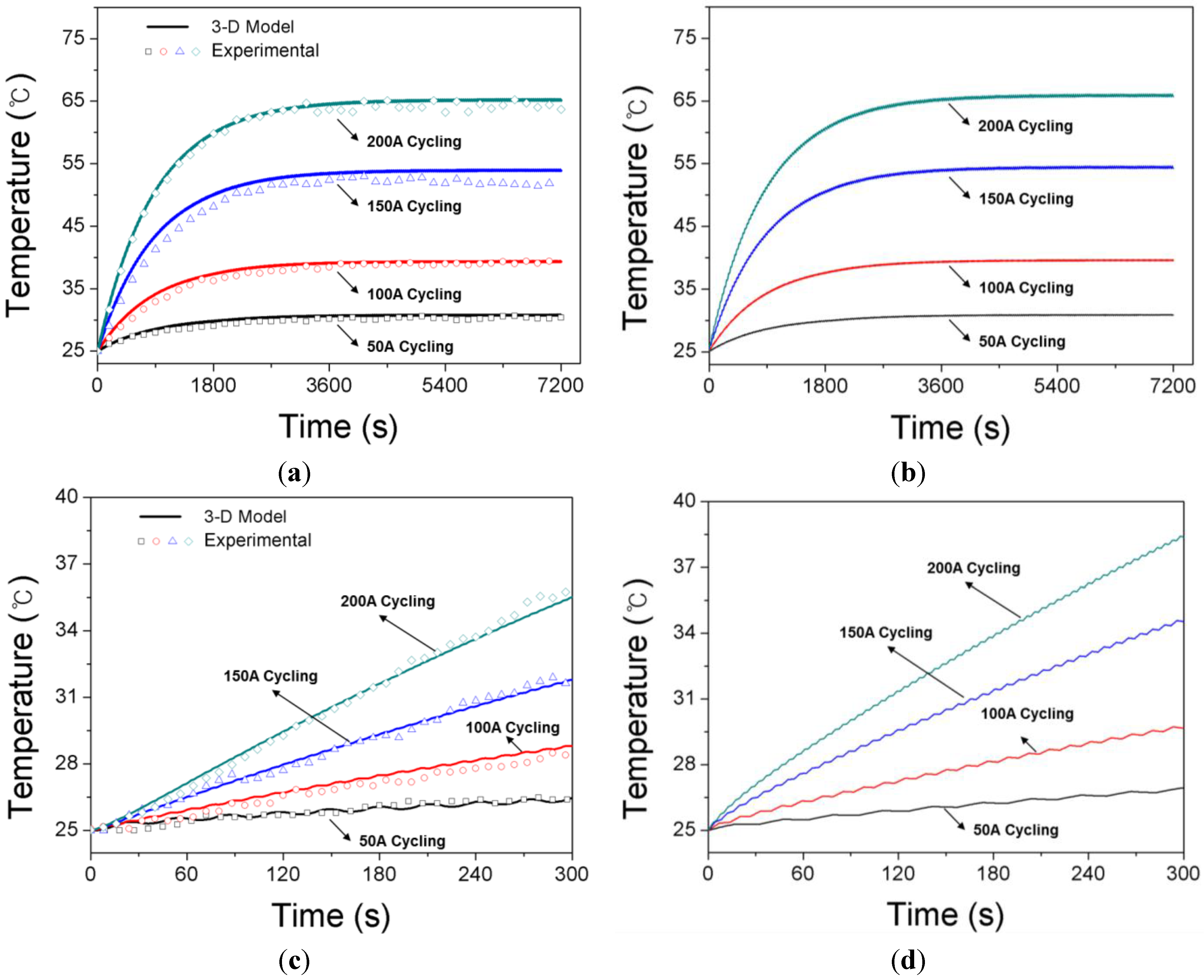
The variations of the surface temperature of the UC case at the middle circumference of the cylindrical UC cell as a function of time predicted by the three-dimensional model are compared with the experimental measurements at various charge/discharge currents of 50, 100, 150, and 200 A in
Figure 7a. To measure the temperature distributions on the surface of battery cell, a thermal imaging infrared camera FLIR T335 (Extech Instruments Corp., Nashua, NH, USA) was used. The IR camera provides 320 × 240 pixels resolution and ±2 °C or ±2% of temperature reading accuracy in the temperature range of −20 °C to 650 °C. The surface temperatures from the experiment and modeling are in good agreement with each other at various charge/discharge currents. The variations of the average temperature of the electrode region (A) of the UC cell as a function of time predicted by the model are plotted at various charge/discharge currents of 50, 100, 150, and 200 A in
Figure 7b. The difference between the calculated average temperature of the electrode region (A) and the surface temperature of the case grows as the charge/discharge current increases. It is about 0.1 °C at the charge/discharge current of 50 A, but it grows up to about 1 °C at the charge/discharge current of 200 A. In
Figure 7c,d, the expanded plots of
Figure 7a,b during the time span from 0 s to 300 s are given to demonstrate the effect of the reversible heating in the model. Although
Figure 7a,b fails to show the effect of the reversible heating due to the time span of
Figure 7a,b, the effect of the reversible heating is clearly reflected in
Figure 7c,d.
Figure 7.
Variations of: (
a) the surface temperature of the UC case; (
b) the temperature of the electrode region (A) as a function of time at various charge/discharge currents of 50, 100, 150, and 200 A; (
c) the expanded plot of
Figure 7a during the time span from 0 s to 300 s; and (
d) the expanded plot of
Figure 7b during the time span from 0 s to 300 s.
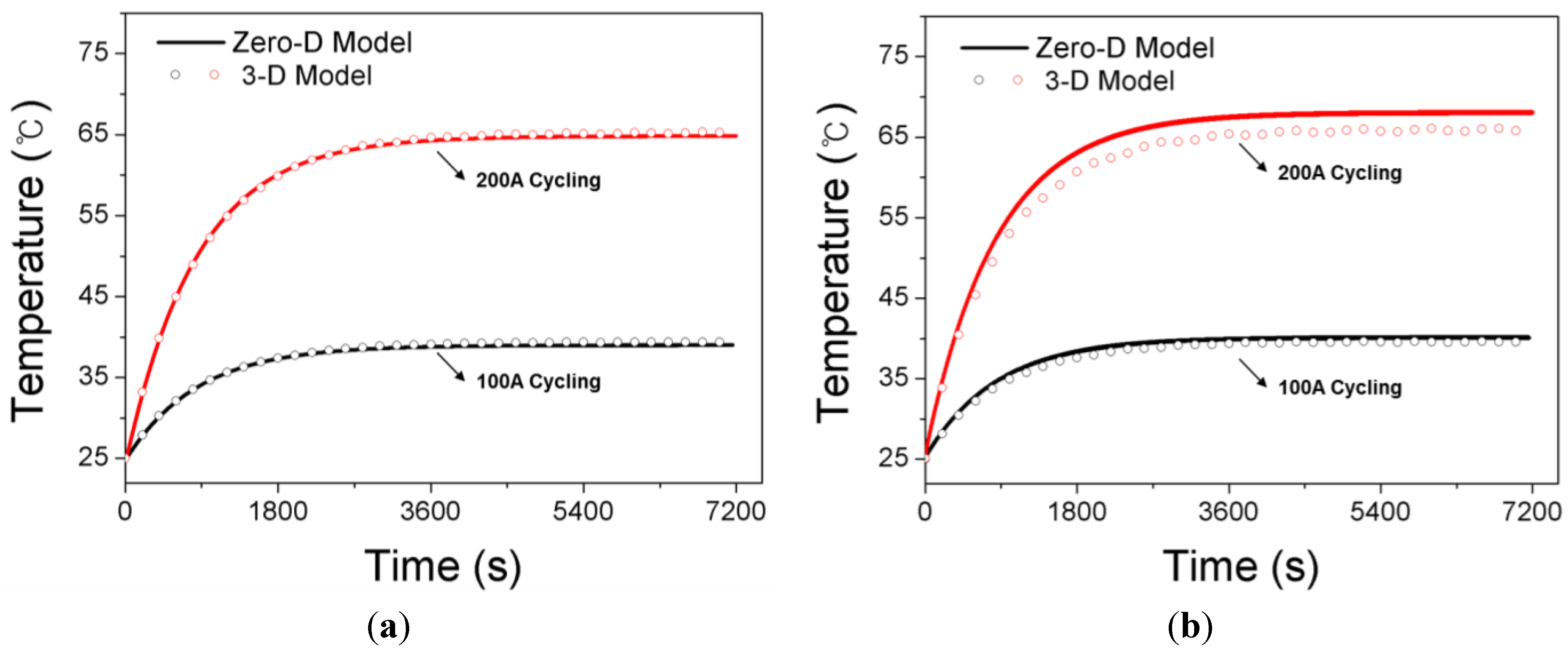
As mentioned in the previous section, the three-dimensional thermal model requires significant computing resources, even though it provides the detailed temperature distribution inside the UC cell. For the purpose of building up a real-time optimal controller of the thermal management system of the UC for automotive applications, a simple zero-dimensional thermal model is proposed in this work. The variations of the surface temperature of the UC and the temperature of the electrode region (A) based on the zero- and three-dimensional thermal models are plotted as a function of time at the charge/discharge currents of 100 A and 200 A in
Figure 8.
Figure 8.
Comparison between the variations of: (a) the surface temperature of the UC; and (b) the temperature of the electrode region (A) based on the zero- and three-dimensional thermal models as a function of time at various charge/discharge currents of 50, 100, 150, and 200 A.
Figure 8.
Comparison between the variations of: (a) the surface temperature of the UC; and (b) the temperature of the electrode region (A) based on the zero- and three-dimensional thermal models as a function of time at various charge/discharge currents of 50, 100, 150, and 200 A.
In case of the surface temperature of the UC, the temperatures based on the zero- and three-dimensional thermal models agree well with each other. Because the surface temperature from the three-dimensional thermal modeling agrees well with the experimental data as shown in
Figure 5 and
Figure 7a, the surface temperature from the zero-dimensional thermal model can predict the experimental data quite well. In case of the temperature of the electrode region, the temperature calculated by the zero-dimensional thermal model is higher than the average temperature from three-dimensional thermal model. The discrepancy between the two is about 0.5 °C at the charge/discharge current of 100 A and it grows up to about 1 °C at the charge/discharge current of 200 A. This discrepancy between the temperatures of the electrode region (A) based on the zero- and three-dimensional thermal models seems to be caused by two reasons. The first reason is that the zero-dimensional model lumps a three-dimensional object into a point and it inherently cannot provide the information of the temperature distribution. The second reason is that the zero-dimensional model presented in this paper takes into consideration of only the heat transfer resistance in the
z-direction shown in
Figure 1b, although the actual heat transfer occurs along the
z- and
r-directions. As easily conjectured from
Figure 1b, the heat transfer path from the electrode region (A) to the case and terminal region (B) along
r-direction is much shorter than that along z-direction. Because the temperature from the three-dimensional model shown in
Figure 8b is the volume-averaged temperature in the electrode region (A) rather than the maximum temperature and the three-dimensional model includes all the effects of the heat transfer along
z- and
r-directions, the temperature from the zero-dimensional model may be naturally a bit higher the volume-averaged temperature from three-dimensional model. Even though the temperature of the electrode region (A) based on the zero-dimensional thermal modeling may be slightly different from that based on the three-dimensional thermal modeling, the surface temperature of the UC from zero-dimensional thermal modeling is as accurate as that from three-dimensional thermal modeling. The zero-dimensional thermal modeling appears adequate for investigating the thermal management issues of the UC for automotive applications, since it does not rely on detailed and computationally intensive numerical simulations. Even though the three-dimensional and zero-dimensional models deal with a cylindrical 2.7 V/650 F UC cell, the modeling approach presented in this work can accommodate the UC cells with different configurations. If the UC cells with different capacities but with the cell components composed of the same materials are to be modeled, the new parameter values of
Table 1 and
Table 3 have to be estimated according to the methods to obtain the parameter values described in this paper. The parameter values of
Table 2 can still be used without any modification. If the UC cell of different shape is to be modeled, the computational mesh and the material properties have to be changed accordingly in case of the three-dimensional model. For the zero-dimensional model, the parameter values of
Table 3 and the thermal resistances of Equations (17) and (18) have to be calculated for the cell of the different shape according to the methods to obtain the parameter values described in this paper.


