Point Estimate Method for Voltage Unbalance Evaluation in Residential Distribution Networks with High Penetration of Small Wind Turbines

Abstract

Voltage unbalance (VU) in residential distribution networks (RDNs) is mainly caused by load unbalance in three phases, resulting from network configuration and load-variations. The increasing penetration of distributed generation devices, such as small wind turbines (SWTs), and their uneven distribution over the three phases have introduced difficulties in evaluating possible VU. This paper aims to provide a three-phase probabilistic power flow method, point estimate method to evaluate the VU. This method, considering the randomness of load switching in customers’ homes and time-variation in wind speed, is shown to be capable of providing a global picture of a network’s VU degree so that it can be used for fast evaluation. Applying the 2m + 1 scheme of the proposed method to a generic UK distribution network shows that a balanced SWT penetration over three phases reduces the VU of a RDN. Greater unbalance in SWT penetration results in higher voltage unbalance factor (VUF), and cause VUF in excess of the UK statutory limit of 1.3%.

1. Introduction

Voltage unbalance (VU) is a costly and potentially damaging phenomenon in electrical power systems. VU will affect network losses, the performance of transformers and induction motors, causing overheating, etc. VU is more common in residential distribution networks (RDNs), where a large number of single-phase loads are used. In RDNs, wherever possible, efforts are made to distribute the single-phase loads uniformly over the three-phase supply. It is recognised that it is unlikely that, at a given time instant, electrical loads are balanced in three phases because of the randomness of load switching in customers’ homes [1]. Load unbalance is the major cause of VU in existing RDNs [2,3]. With integration of distributed power generating equipment, such as small wind turbines (SWTs), VU scenarios will change due to the additional power injected at distributed points across the network. This will have increasing impact and importance as SWTs are expected to reach a high penetration level in RDNs over the next two decades [4]. The time-varying output power of SWTs will impact on power required from the RDN’s grid connection point, and consequently impact on voltage variation through the system. This has introduced more difficulties in evaluating VU in RDNs.

As stipulated in Engineering Recommendation G83/2 [5], distributed generation (DG) units rated up to 16 A per phase can be connected to low voltage (LV) networks. In this paper SWTs refer to single-phase, induction machine based, wind turbines, i.e. at 230 V a.c. (alternating current) they are rated less than 3.68 kVA. For simplicity, all the residential-scale SWTs have been taken as 3.5 kVA.

In a three-phase system, the degree of VU is expressed by the ratio (in per cent) between the root mean square (rms) values of the negative and positive sequence voltage components. This ratio is termed as the voltage unbalance factor (VUF). According to UK Engineering Recommendation P29 [6], the VUF at the load point should be kept within 1.3% and short term deviations (less than 1 min) should not exceed 2%.

When evaluating VU in distribution networks with DG, the three-phase loads were considered as having constant values in [7,8]. For instance, in [7], loads in phase A, B and C were assumed to be 60, 120 and 180 kW, respectively. The time varying characteristics of loads should be considered. Moreover, with SWT systems, the time-varying power injection from SWTs can change either, or both, magnitude and direction of a network’s power flow. The time-variation in SWT output power should also be considered. Therefore, the application of the time series method (TSM) to power flow analysis can be advantageous [9,10,11,12]. For detailed analysis, a specific time window with a period of a day or a week is usually used. However, the specific time windows cannot provide a global picture of VU and, consequently, cannot indicate the severity of VU of a network under study [13].

A probabilistic analysis, able to capture the effect of the time varying characteristics but requiring lower computational power, could provide a more realistic study than the TSM [14]. Techniques such as Monte Carlo simulation (MCS) [1,15] and approximate method [16,17] have been used for the probabilistic power flow (PPF) analysis of VU. MCS is time consuming as a large number of simulations, e.g., 20,000, are required. To reduce the computational power, an approximate method, point estimate method (PEM), was used in studies [16,17,18,19]. The PEM uses deterministic procedures to solve probabilistic problems through only a few first statistical moments of probability functions, such as mean and variance, of input variables. The PEM calculation can approximate the exact mean of the output quantity of interest.

In [16], the PEM was used to evaluate the steady operating condition of an unbalanced power system. In this study, the uncertainties (variables) considered were load variation, line/cable parameters and generator unit outage, but the impact of DG was not included. The presence of wind farms was considered in [17]. This paper had two three-phase (balanced) wind turbines integrated into an unbalanced distribution network. However, for SWTs it is more likely single-phase units are installed. In addition, the penetration among three phases is not expected to be perfectly uniform. As this could result in uneven power generation over the three phases, different SWT penetration and distribution scenarios should be considered for the VU studies.

For the PEM, different schemes can be used, including 2m, 2m + 1, and 4m +1 schemes, where m is the number of input variables. The 2m + 1 scheme is considered in this paper, as it was shown to have good performance in terms of both accuracy and computational time [16,17].

In this paper, the VU in RDNs with different SWT penetration and distribution scenarios has been evaluated by using the PEM. The randomness of switching of loads and the time-varying characteristics of wind speeds have been taken into account. The proposed methodology, proved capable of providing a global picture on VU probabilities particularly in comparison with TSM approach, has the potential to be used for fast evaluation. This will enable distribution network operators (DNOs) to quantify, in a statistical manner, the VU of the three-phase nodes in a RDN.

2. System Modelling and Problem Formulation

To evaluate VU in RDNs, variation of loads and variation of power generated by SWTs due to variation in wind speed should be modelled. The processes for each, and the problem formulation, are presented in the following sections.

2.1. Load Modelling

Node voltages in a distribution network, related to active and reactive power flow in branches, can be obtained via steady-state power flow analysis. The power flow depends on the instantaneous aggregation of the individual electrical demands of many customers. Due to the time varying characteristics of the loads, it is usually necessary to model system loads on a statistical basis [2].

The daily residential load profiles used in [20] are adopted for the load modelling in this paper. At a time instant of the day, the aggregated load in each of the three phases is considered as a random variable (three variables in total). Each variable is then discretized and can be expressed as discrete values with their corresponding probabilities, as shown in Equation (1):

$$F_{L_{\text{α}}}=\{L_{\text{α}}\left(j\right),F_{L_{\text{α}}}\left(j\right):j=1,2,\dots ,W\}$$

(1)

where α = A, B or C, refers to the phase specified; Lα(j) is the discrete value of the sum of loads in phase α, and $W$ is the number of discrete values; $F_{L_{\text{α}}}$ is the corresponding probability of loads at discrete value L_α(j).

At each time instant, the mean and standard deviation of the sum of loads in phase α can be expressed as ${\text{μ}}_{L_{\text{α}}}$ and ${\text{σ}}_{L_{\text{α}}}$, respectively:

$${\text{μ}}_{L_{\text{α}}}={\displaystyle \sum }_{j=1}^W{L}_{\text{α}}\left(j\right)\times F_{L_{\text{α}}}\left(j\right),j=1,2,\dots ,W$$

(2)

$${\text{σ}}_{L_{\text{α}}}=\sqrt{{\displaystyle \sum }_{j=1}^W{[L_{\text{α}}\left(j\right)]}^2\times F_{L_{\text{α}}}\left(j\right)-{({\text{μ}}_{L_{\text{α}}})}^2},j=1,2,\dots ,W$$

(3)

2.2. SWT Output Power Modelling

Due to the intermittent characteristic of wind speed, SWT output is neither continuous nor stable. The Weibull distribution function is widely used to statistically describe the wind speed distribution, e.g., [21,22]. The statistical SWT model used in [13] is employed in this work. All wind speed data at a specific time of the day is differentiated into discrete values. With a given SWT power output curve, the discrete SWT outputs and the corresponding probabilities can be obtained, as seen in Equation (4):

$$F_G=\{P_G\left(i\right),F_G\left(i\right):i=0,1,2,\dots ,M\}$$

(4)

where the SWT output power $P_G\left(i\right)$ has $M+1$ states at which the probability of $P_G\left(i\right)$ is calculated from the discrete wind speeds and the SWT power output curve. $F_G\left(i\right)$ is the probability of SWT output for the $i$th SWT output value, as shown in Figure 1. $M$ has been taken as 10 in the figure.

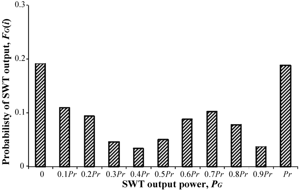
Figure 1. The probabilistic distribution of SWT output power, M = 10.

Figure 1. The probabilistic distribution of SWT output power, M = 10.

At each time instant, the mean and standard deviation of the SWT output power can be expressed as ${\text{μ}}_{P_G}$ and ${\text{σ}}_{P_G}$, respectively:

$${\text{μ}}_{P_G}={\displaystyle \sum }_{i=0}^M{P}_G\left(i\right)\times F_G\left(i\right),i=0,1,\dots ,M$$

(5)

$${\text{σ}}_{P_G}=\sqrt{{\displaystyle \sum }_{i=0}^M{[P_G\left(i\right)]}^2\times F_G\left(i\right)-{({\mu }_{P_G})}^2},i=0,1,\dots ,M$$

(6)

2.3. Problem Formulation

For a given network, the line/cable parameters are assumed to be fixed. Due to the area of a RDN, it is also assumed that, at a given time the wind speed is the same for all SWT systems. This means that the output power from all SWTs, disregarding the connection phase, can be considered as one variable. Therefore, the voltage unbalance factor (VUF) is determined by four random variables: loads in phase A, B, C ($L_A$, $L_B$, $L_C$) and the output power from a single SWT ($P_G$), which can be mathematically described by Equation (7):

$$VUF\propto h(L_A,L_B,L_C,P_G)$$

(7)

where $h$ is a nonlinear function defined by a power flow analysis and a calculation of the $VUF$ using the results obtained by the power flow analysis.

By adopting the PEM method, specific values of $L_A$, $L_B$, $L_C$ and $P_G$ will be provided for the power flow analysis. Details of the determination of these values will be presented in Section 3. Once the complex vectors (including magnitude and angle) of the phase voltages ($\dot{V_A}$, $\dot{V_B}$ and $\dot{V_C}$) are obtained by the power flow analysis, the $VUF$ can be calculated using the Equation (8) [6]:

$$VUF=\frac{\left|{\dot{V}}^{(2)}\right|}{\left|{\dot{V}}^{(1)}\right|}\times 100\%$$

(8)

where ${\dot{V}}^{(2)}$ and ${\dot{V}}^{(1)}$ are the complex negative and positive sequence voltages, respectively. ${\dot{V}}^{\left(2\right)}=\dot{V_A}+\dot{V_B}\times {(e^{j2\text{π}/3})}^2+\dot{V_C}\times e^{j2\text{π}/3}$, $V^{\left(1\right)}=\dot{V_A}+\dot{V_B}\times e^{j2\text{π}/3}+\dot{V_C}\times {(e^{j2\text{π}/3})}^2$.

3. Methodology

This section presents the details of using the 2m + 1 scheme of the PEM for the VU evaluation. The specific values (points) for the four variables and the corresponding weighing factors are determined. The overall computational procedure for the $VUF$ evaluation is also presented.

3.1. Application of the Point Estimate Method (PEM)

This paper employs the 2m + 1 scheme of the PEM. Once the mean of the four variables which determine the $VUF$, i.e., ${\text{μ}}_{L_A}$, ${\text{μ}}_{L_B}$, ${\text{μ}}_{L_C}$ and ${\text{μ}}_{P_G}$, and their standard deviations, i.e., ${\text{σ}}_{L_A}$, ${\text{σ}}_{L_B}$, ${\text{σ}}_{L_C}$ and ${\text{σ}}_{P_G}$, are obtained by applying Equations (1)–(6), two points for each variable can be calculated using Equation (9):

$$\begin{array}{l}{L}_{A, q}={\text{μ}}_{L_A}+{\text{ξ}}_{L_{A, q}}\times {\text{σ}}_{L_A}\\ L_{B, q}={\text{μ}}_{L_B}+{\text{ξ}}_{L_{B, q}}\times {\text{σ}}_{L_B}\\ L_{C, q}={\text{μ}}_{L_C}+{\text{ξ}}_{L_{C, q}}\times {\text{σ}}_{L_C}\\ P_{G, q}={\text{μ}}_{P_G}+{\text{ξ}}_{P_{G, q}}\times {\text{σ}}_{P_G}& \left(q=1, 2\right)\end{array}$$

(9)

where ${\text{ξ}}_{m, q}=\frac{{\text{λ}}_{m, 3}}{2}+{(-1)}^{3-q}\sqrt{{\text{λ}}_{m, 4}+\frac{3}{4}\times {({\text{λ}}_{m, 3})}^2}$, $q$ = 1, 2; $m$ is one of the four variables ($L_A$, $L_B$, $L_C$ or $P_G$). ${\text{λ}}_{m, 3}$ and ${\text{λ}}_{m, 4}$ denote the third and fourth standard central moments of the input variable m. They are calculated as follows:

$$\begin{array}{l}{\text{λ}}_{m, 3}=\frac{E[{(m-{\text{μ}}_m)}^3]}{{({\text{σ}}_m)}^3}\\ {\text{λ}}_{m, 4}=\frac{E[{(m-{\text{μ}}_m)}^4]}{{({\text{σ}}_m)}^4}\end{array}$$

(10)

where $E\left[{\left(m-{\text{μ}}_m\right)}^3\right]={\displaystyle \sum }_{t=1}^Z{(m_{,t}-{\text{μ}}_m)}^3\times Prob(m_{,t})$ and $E\left[{\left(m-{\text{μ}}_m\right)}^4\right]={\displaystyle \sum }_{t=1}^Z{(m_{,t}-{\text{μ}}_m)}^4\times Prob(m_{,t})$. $Prob\left(m_{,t}\right)$ is the probability of each discrete value of $m$. $Z$ is the total number of the discrete values of $m$. For variables $L_A$, $L_B$ and $L_C$, $Z$ is equal to $W$, and for variable $P_G$, $Z$ is equal to $M+1$.

The weighting factor for each point of the four variables can be expressed by Equation (11):

$${\text{ω}}_{m, q}={(-1)}^q\frac{1}{{\text{ξ}}_{m, q}({\text{ξ}}_{m,1}-{\text{ξ}}_{m, 2})}, q=1, 2$$

(11)

where ${\text{ω}}_{m, q}$ ranges from 0 to 1 corresponding to the specific point shown in Equation (9).

Once the specific value representing the aggregated phase load is determined, this value is evenly distributed and assigned to each customer in the corresponding phase. For the SWT output power, the calculated value is applied to all SWTs in the network. With these assigned values, the power flow analysis is carried out. In the sequence, the $VUF$ for each corresponding point can be calculated by Equation (8).

The 2m + 1 scheme requires a further run of power flow analysis and $VUF$ calculation with the means of all input variables. The corresponding weighing factor of this calculation is obtained by Equation (12):

$${\text{ω}}_0=1-{{\displaystyle \sum }}^{\text{}}\frac{1}{{\text{λ}}_{m, 4}-{\left({\text{λ}}_{m,3}\right)}^2}$$

(12)

where $m$ is one of the four variables ($L_A$, $L_B$, $L_C$ or $P_G$). ${\text{ω}}_0$ ranges from 0 to 1. The sum of all ${\text{ω}}_{m, q}$ and ${\text{ω}}_0$ is unity.

Then the mean of the $VUF$ and mean of ${[h(L_A, L_B, L_C, P_G)]}^2$ can be obtained by Equations (13) and (14):

$$\begin{array}{l}E\left(VUF\right)=E\left[h\left(L_A, L_B, L_C, P_G\right)\right]\\ \cong {\text{ω}}_{L_A, 1}\times h\left(L_{A, 1},{\text{μ}}_{L_B}, {\text{μ}}_{L_C}, {\text{μ}}_{P_G}\right)+{\text{ω}}_{L_A, 2}\times h\left(L_{A, 2},{\text{μ}}_{L_B}, {\text{μ}}_{L_C}, {\text{μ}}_{P_G}\right)\\ +{\text{ω}}_{L_B, 1}\times h({\text{μ}}_{L_A},L_{B, 1}, {\text{μ}}_{L_C}, {\text{μ}}_{P_G})+{\text{ω}}_{L_B, 2}\times h({\text{μ}}_{L_A},L_{B, 2}, {\text{μ}}_{L_C}, {\text{μ}}_{P_G})\\ +{\text{ω}}_{L_C, 1}\times h\left({\text{μ}}_{L_A}, {\text{μ}}_{L_B}, L_{C, 1}, {\text{μ}}_{P_G}\right)+{\text{ω}}_{L_C, 2}\times h\left({\text{μ}}_{L_A}, {\text{μ}}_{L_B}, L_{C, 2}, {\text{μ}}_{P_G}\right)\\ +{\text{ω}}_{P_G, 1}\times h\left({\text{μ}}_{L_A}, {\text{μ}}_{L_B}, {\text{μ}}_{L_C}, P_{G, 1}\right)+{\text{ω}}_{P_G, 2}\times h\left({\text{μ}}_{L_A}, {\text{μ}}_{L_B}, {\text{μ}}_{L_C}, P_{G, 2}\right)\\ +{\text{ω}}_0\times h\left({\text{μ}}_{L_A}, {\text{μ}}_{L_B}, {\text{μ}}_{L_C}, {\text{μ}}_{P_G}\right)\end{array}$$

(13)

$$\begin{array}{l}E\left\{{\left[h\left(L_A, L_B, L_C, P_G\right)\right]}^2\right\}\\ \cong {\text{ω}}_{L_A, 1}\times {\left[h\left(L_{A, 1},{\text{μ}}_{L_B}, {\text{μ}}_{L_C}, {\text{μ}}_{P_G}\right)\right]}^2+{\text{ω}}_{L_A, 2}\times {\left[h\left(L_{A, 2},{\text{μ}}_{L_B}, {\text{μ}}_{L_C}, {\text{μ}}_{P_G}\right)\right]}^2\\ +{\omega }_{L_B, 1}\times {\left[h\left({\text{μ}}_{L_A},L_{B, 1}, {\text{μ}}_{L_C}, {\text{μ}}_{P_G}\right)\right]}^2+{\text{ω}}_{L_B, 2}\times {\left[h\left({\text{μ}}_{L_A},L_{B, 2}, {\text{μ}}_{L_C}, {\text{μ}}_{P_G}\right)\right]}^2\\ +{\omega }_{L_C, 1}\times {\left[h\left({\text{μ}}_{L_A}, {\text{μ}}_{L_B}, L_{C, 1}, {\text{μ}}_{P_G}\right)\right]}^2+{\omega }_{L_C, 2}\times {\left[h\left({\text{μ}}_{L_A}, {\text{μ}}_{L_B}, L_{C, 2}, {\text{μ}}_{P_G}\right)\right]}^2\\ +{\omega }_{P_G, 1}\times {\left[h\left({\text{μ}}_{L_A}, {\text{μ}}_{L_B}, {\text{μ}}_{L_C}, P_{G, 1}\right)\right]}^2+{\omega }_{P_G, 2}\times {[h\left({\text{μ}}_{L_A}, {\text{μ}}_{L_B}, {\text{μ}}_{L_C}, P_{G, 2}\right)]}^2\\ +{\omega }_0\times {\left[h\left({\text{μ}}_{L_A}, {\text{μ}}_{L_B}, {\text{μ}}_{L_C}, {\text{μ}}_{P_G}\right)\right]}^2\end{array}$$

(14)

The standard deviation of the $VUF$ can be obtained by Equation (15):

$${\text{σ}}_{VUF}=\sqrt{E\left\{{\left[h\left(L_A, L_B, L_C, P_G\right)\right]}^2\right\}-{\left\{E\left[h\left(L_A, L_B, L_C, P_G\right)\right]\right\}}^2}$$

(15)

3.2. Overall Calculation Procedure

The power flow analysis is carried out adopting a one-day or daily 24-h period with half-an-hour per step. The overall computational procedure for the VU evaluation is depicted in Figure 2. First, the SWT penetration is assigned to each of the three phases prior to a power flow analysis. At the nth half-hour of the day, the four variables ($L_A$, $L_B$, $L_C$ and $P_G$) are then differentiated into discrete values, and the mean and standard deviation of these variables are calculated. This corresponds to Equations (1)–(6). Thereafter, two points for each of the four variables and the corresponding weighting factors are determined using Equations (9) and (11). These points are assigned to each customer and SWT system in the network accordingly, with which the power flow analyses are carried out. In addition, $VUF$ calculation using the means of all input variables is carried out considering the corresponding weighting factor. In the sequence, the $VUF$ for the nth half-hour $E_n\left(VUF\right)$ is obtained by nine simulation-runs and the calculation using Equation (13). The system repeats this process for every time step until it finishes the simulation for the last half-hour of the day.

Figure 2. Overall computational procedure of the proposed methodology.

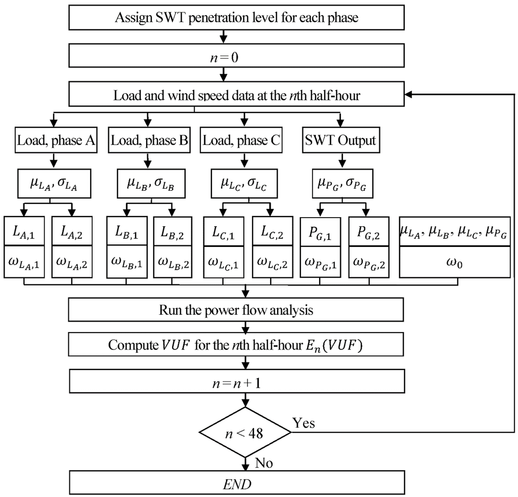
Figure 2. Overall computational procedure of the proposed methodology.

4. Case Study

4.1. Example Distribution Network Model

The proposed methodology is applied to a generic UK distribution network, based on data in [8]. DIgSILENT Powerfactory software (DIgSILENT GmbH, Gomaringen, Germany) is used to simulate the system.

The 33/11 kV network is comprised of six 11 kV radial feeders. Each feeder supplies eight 11 kV/400 V 500 kVA transformers. Five of the 11 kV feeders are modelled as lumped loads, whilst the sixth is presented in details, Figure 3. One of the 400 V sub-networks on the sixth feeder is modified to represent a RDN (with 3-phase 4-wire underground cables). The three-phase nature and single-phase connections of customer loads and SWTs are considered. There are 110, 150 and 130 houses, respectively, in the three phases (i.e., 390 in total), all with a power factor (pf) of 0.98. As shown in Figure 3 each L represents 10 houses. SWTs, rated at 3.5 kVA with a pf of 0.95, are installed in a proportion of the houses. The simulations reported focus on the VU at the secondary of the 11 kV/400 V transformer (e.g., LV busbar) and the nodes along the LV cables.

Figure 3. A generic UK distribution network with SWTs (reproduced from [8]).

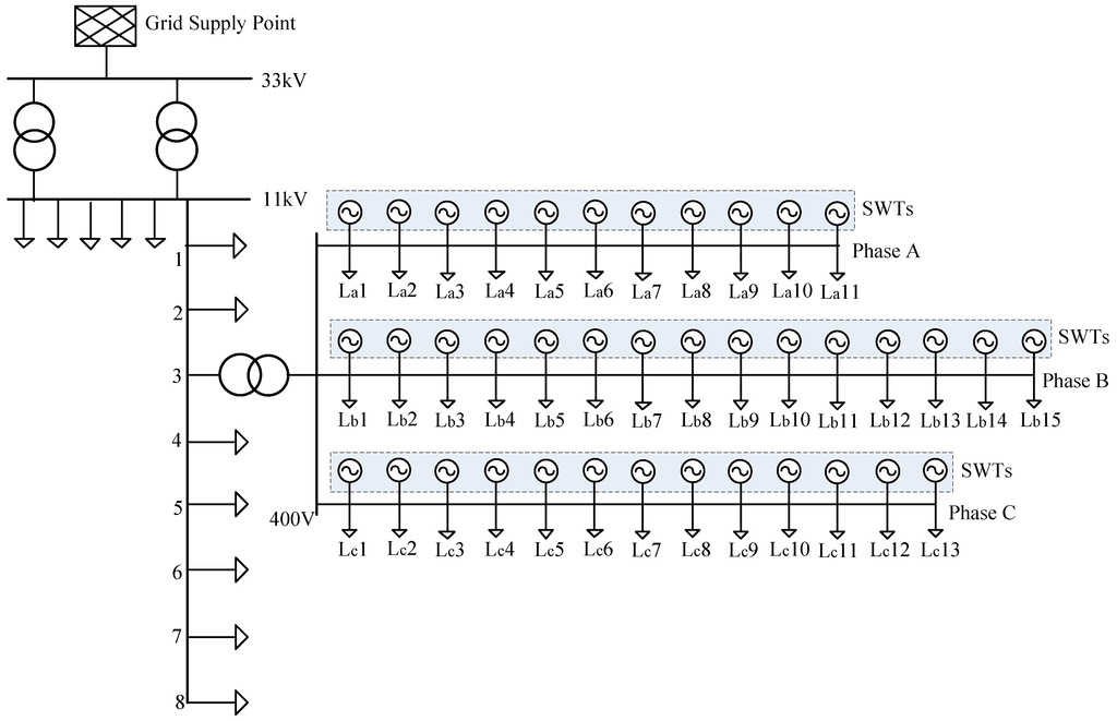
Figure 3. A generic UK distribution network with SWTs (reproduced from [8]).

4.2. Simulation Scenarios

In this paper, the SWT penetration is calculated by the number of houses having SWT systems installed in relation to the total number of houses in the corresponding phase, i.e., for a penetration of 40%, 44 out of 110 houses in phase A have SWTs installed. As SWTs can be evenly or unevenly distributed, five scenarios are considered, see Table 1. The highest penetration in this paper is 40%, which considers the cumulative penetration and is a possible projection for a small scale area in a future RDN [4].

Table 1. Simulation scenarios.

Scenario	SWT distribution	SWT penetration level			SWT capacity to the 11 kV/400 V transformer rating
		Phase A	Phase B	Phase C
1	No SWTs	0	0	0	0
2	Balanced	20%	20%	20%	54.6%
3	Balanced	40%	40%	40%	109.2%
4	Unbalanced	40%	20%	0	51.8%
5	Unbalanced	40%	0	0	30.8%

Table 1. Simulation scenarios.

Scenario	SWT distribution	SWT penetration level			SWT capacity to the 11 kV/400 V transformer rating
		Phase A	Phase B	Phase C
1	No SWTs	0	0	0	0
2	Balanced	20%	20%	20%	54.6%
3	Balanced	40%	40%	40%	109.2%
4	Unbalanced	40%	20%	0	51.8%
5	Unbalanced	40%	0	0	30.8%

5. Simulation Results and Discussion

5.1. Simulation Results

Based on half-hourly domestic (un-restricted) load data from 2004 [18] and wind speed data in Camborne, UK for the same year [23], steady state three-phase power flow analyses are executed and $VUF$ values are calculated. Figure 4 and Figure 5 show the daily probabilistic mean value of $VUF$s for the five scenarios simulated: Scenario 1 has been included in both figures for comparison purpose. In each Figure (a) relates to $VUF$ at the secondary of the 11 kV/400 V transformer (e.g., LV busbar) and (b) relates to $VUF$ at the remote end of the LV cables.

Figure 4a illustrates that, for the cases where SWT penetration is balanced across the three phases (Scenarios 2 and 3), the $VUF$ reduces with increasing penetration of SWTs, compared to Scenario 1 (no SWTs); for the cases with unbalanced distribution of SWTs (Scenarios 4 and 5), the VUFs are higher than in Scenario 1, as shown in Figure 5a, and the VU in Scenario 5 is the worst-case scenario. For each scenario, VUFs at the remote end of the LV cables are shown higher than the LV busbar.

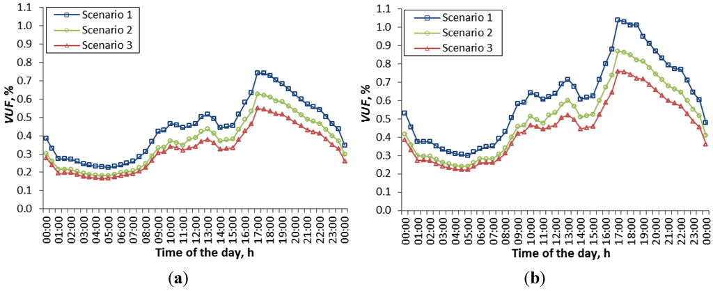
Figure 4. VUFs for balanced SWT penetration at: (a) the LV busbar and (b) the remote end of the LV cables.

Figure 4. VUFs for balanced SWT penetration at: (a) the LV busbar and (b) the remote end of the LV cables.

Figure 5. VUFs for unbalanced SWT penetration at: (a) the LV busbar and (b) remote end of the LV cables.

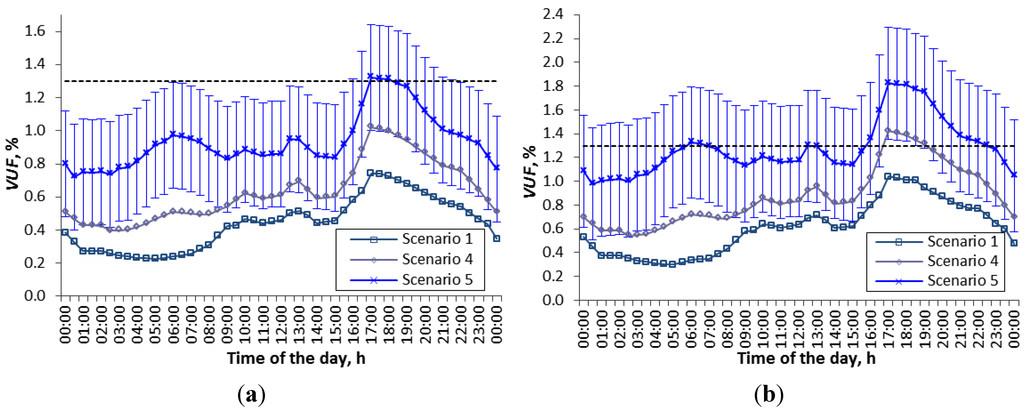
Figure 5. VUFs for unbalanced SWT penetration at: (a) the LV busbar and (b) remote end of the LV cables.

The $VUF$ is most likely to exceed the UK statuary limit of 1.3% in the following cases:

• Scenario 4—at the remote end of the LV cables during the peak load hours (17:00 to 19:30);
• Scenario 5—at the LV busbar during peak load hours (17:00 to 19:00);
• Scenario 5—at the remote end of LV cables during the hours (5:00 to 7:30), (12:30 to 13:00) and peak load hours (15:30 to 23:00).

By using PEM, the standard deviation of the VUF at each time step of the five simulated scenarios can also be obtained using Equation (15). The standard deviation will help to show the possible range of the $VUF$. For instance, error bars in Figure 5 demonstrate the standard deviations in simulation Scenario 5. At the LV busbar, the possible $VUF$ can be the mean value ± 0.32% (Note that the $VUF$ value is in percentage.); at the remote end of the LV cables, the $VUF$ can be the mean value ± 0.51%. The average standard deviations of the $VUF$ for the five simulation scenarios are shown Table 2. This gives a possible range of the corresponding $VUF$s, but the actual values are not limited to the range.

Table 2. Average standard deviations of the $VUF$ for the five simulation scenarios.

Scenarios	The LV busbar	Remote end
1	0.19%	0.27%
2	0.21%	0.36%
3	0.20%	0.32%
4	0.28%	0.45%
5	0.32%	0.51%

Table 2. Average standard deviations of the $VUF$ for the five simulation scenarios.

Scenarios	The LV busbar	Remote end
1	0.19%	0.27%
2	0.21%	0.36%
3	0.20%	0.32%
4	0.28%	0.45%
5	0.32%	0.51%

To examine the VU a distribution network experiences at different loading conditions, correlation between the percentage of the peak load and VUFs at the LV busbar were sought. The correlation is represented by a linear trend for each simulated scenario, as illustrated in Figure 6. The trend suggested in Figure 4 and Figure 5, i.e., higher VUF exists for greater unbalance in SWT penetration, is also indicated here and Scenario 5 is shown to be the worst-case scenario among all the scenarios.

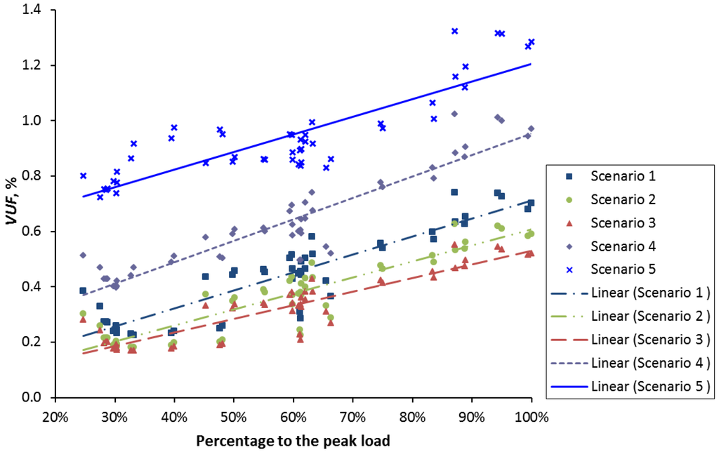
Figure 6. Correlation between percentage of peak load and VUFs at the LV busbar.

Figure 6. Correlation between percentage of peak load and VUFs at the LV busbar.

Although this work employs a PPF analysis method, the minimum and maximum loads for the simulated scenarios should be checked to ensure they do not exceed the rating of the corresponding transformers. Table 3 shows the loadings of the 11 kV/400 V transformer at different times of the day. Note that the loads at 01:00 and 18:30 are the lowest and the highest of the day, respectively. “*” in Table 3 denotes the power flow from the load side upstream to the grid supply point.

Table 3. 11 kV/400 V transformer loadings at different times of the day.

Scenario	01:00 am		11:00 am		18:30 pm		22:00 pm
	Min	Max	Min	Max	Min	Max	Min	Max
1	9.5%	58.2%	12.5%	65.4%	26.8%	96.5%	19.6%	79.4%
2	40.6%*	58.2%	37.9%*	65.4%	25.0%*	96.5%	31.5%*	79.4%
3	87.7%*	58.2%	85.1%*	65.4%	72.5%*	96.5%	78.8%*	79.4%
4	33.8%*	58.2%	31.4%*	65.4%	18.1%*	96.5%	25.8%*	79.4%
5	14.9%*	58.2%	12.8%*	65.4%	1.7%*	96.5%	7.8%*	79.4%

Table 3. 11 kV/400 V transformer loadings at different times of the day.

Scenario	01:00 am		11:00 am		18:30 pm		22:00 pm
	Min	Max	Min	Max	Min	Max	Min	Max
1	9.5%	58.2%	12.5%	65.4%	26.8%	96.5%	19.6%	79.4%
2	40.6%*	58.2%	37.9%*	65.4%	25.0%*	96.5%	31.5%*	79.4%
3	87.7%*	58.2%	85.1%*	65.4%	72.5%*	96.5%	78.8%*	79.4%
4	33.8%*	58.2%	31.4%*	65.4%	18.1%*	96.5%	25.8%*	79.4%
5	14.9%*	58.2%	12.8%*	65.4%	1.7%*	96.5%	7.8%*	79.4%

5.2. Comparison between PEM and TSM

When using PEM, errors may be introduced in the process of discretizing the load and wind speed data, e.g. a wind speed 6.4 m/s may be considered as 6 m/s, depending on the chosen discrete values and the width of the speed range. Moreover, although the PEM provides good estimates, error exists due to the estimation characteristics of the PEM.

TSM is a method carrying out power flow analyses in time series with specific values of system load and SWT output power for each time step. This method is accurate as the actual load and SWT output values can be used in the power flow simulations. In this paper, the results of the mean VUFs obtained by PEM are compared with those from the TSM (Table 4).

Taking the results of the TSM as reference, Table 3 demonstrates that the maximum error introduced by using PEM is 10.9%. In terms of the required computing power, at any time of the day, 9 power flow simulations are needed when using PEM. This is only approximately 2.5% of that the TSM requires, which is 1 power flow simulation (for this specific time of a day) per day over 365 days.

In terms of sampling intervals, a half-hourly resolution is used in this paper. A higher resolution, e.g., 1-min, increases the accuracy of the simulation results. However, when the same sample interval is used by the PEM and TSM, the former requires approximately 2.5% of the computing power that used by the latter.

In addition, the daily probabilistic mean of the VUFs resulting from the PEM provide a global picture of VU probabilities and the likelihood of these values. Nevertheless, PEM has its disadvantages that unlike TSM, the PEM cannot provide a deterministic time-series VUF profile of a node in a network for a specified time frame.

Table 4. VUFs comparison by using PEM and TSM.

Scenario	Time of the day	VUF, %
		LV busbar			Remote end
		TSM	PEM	Difference	TSM	PEM	Difference
1	1:00	0.268	0.273	1.9%	0.383	0.375	−2.1%
	11:00	0.425	0.442	4.0%	0.612	0.606	−1.0%
	18:30	0.668	0.702	5.1%	1.076	1.012	−5.9%
	22:00	0.523	0.541	3.4%	0.827	0.770	−6.9%
3	1:00	0.187	0.194	3.7%	0.259	0.273	5.4%
	11:00	0.338	0.320	−5.3%	0.481	0.444	−7.7%
	18:30	0.480	0.518	7.9%	0.824	0.722	−12.4%
	22:00	0.393	0.412	−8.6%	0.547	0.569	−9.9%
5	1:00	0.821	0.750	10.7%	1.116	1.005	10.2%
	11:00	0.768	0.850	8.1%	1.053	1.160	10.9%
	18:30	1.188	1.284	6.8%	1.598	1.772	−1.1%
	22:00	0.908	0.970	1.9%	1.347	1.332	−2.1%

“TSM” denotes Times Series Method; “PEM” Point Estimate Method.

Table 4. VUFs comparison by using PEM and TSM.

Scenario	Time of the day	VUF, %
		LV busbar			Remote end
		TSM	PEM	Difference	TSM	PEM	Difference
1	1:00	0.268	0.273	1.9%	0.383	0.375	−2.1%
	11:00	0.425	0.442	4.0%	0.612	0.606	−1.0%
	18:30	0.668	0.702	5.1%	1.076	1.012	−5.9%
	22:00	0.523	0.541	3.4%	0.827	0.770	−6.9%
3	1:00	0.187	0.194	3.7%	0.259	0.273	5.4%
	11:00	0.338	0.320	−5.3%	0.481	0.444	−7.7%
	18:30	0.480	0.518	7.9%	0.824	0.722	−12.4%
	22:00	0.393	0.412	−8.6%	0.547	0.569	−9.9%
5	1:00	0.821	0.750	10.7%	1.116	1.005	10.2%
	11:00	0.768	0.850	8.1%	1.053	1.160	10.9%
	18:30	1.188	1.284	6.8%	1.598	1.772	−1.1%
	22:00	0.908	0.970	1.9%	1.347	1.332	−2.1%

“TSM” denotes Times Series Method; “PEM” Point Estimate Method.

5.3. Discussion

This paper considered the aggregated phase load as a random variable. The load was assumed to be evenly distributed without considering load diversity of individual customers. Firstly, although the load difference between customers may result in some slightly different voltage drops in segments along the LV feeder, the VU is mainly caused by the net load unbalance, related to the difference in the aggregated phase load. Secondly, this paper aims to find a fast VU evaluation method. Considering the amount of computing power reduced by using PEM, the observed accuracy of up to approximately 11% difference from the results of using TSM is not that bad.

In practice, non-uniform distribution of residential loads is likely, even with the same number of houses connected into each of the three phases, as the electrical demand in each customer’s home is difficult to forecast. DNOs have limited control of short-term variations in VU. Given these factors, as discussed in [6], a background VU may exist, but it rarely exceeds 0.5%, and levels in excess of 1% may be experienced at times of high load and/or when unbalanced loads are distributed. Therefore, the initial load arrangement is based on a configuration which can lead to the maximum $VUF$ of a network without SWT systems. The maximum $VUF$ for the studied RDN using the arrangement, i.e., Scenario 1, is 1.07%, within the UK statutory limit.

All loads considered are single-phase loads. As distribution networks in urban areas contain both residential and commercial loads, it is likely that three-phase loads are present. Further study will consider distribution networks containing some three-phase loads.

The impact of SWTs on VU is mainly from the distributed power injection, in this work a number of assumptions have been made, as outlined below.

One assumption is that at all times the wind speed is the same for all SWTs in the segment of the RDN. It is possible that variations in wind speed could exist, even within the small area of a RDN, due to terrain effects, wind shadows, etc. As an example, the SWT distribution in Scenario 5 could happen if the residences in one phase are suitable for SWT installation, e.g., Phase A homes are all located upon a ridge along a hill, and homes in phases B and C are not suitable for SWT installation, as they are located in the wind shadow of the hill. Without knowing the geographical topology and layout of a given RDN it is not possible to model a specific area, nor feasible to consider all options. If the methodology is shown to be valid for this assumed arrangement then utilities would be able to expand the parameter base to include these effects. It is expected that diversity in wind distribution would create wider (or more diversified) differences in power production from SWTs in the three phases.

A second assumption made is that the pf of all SWTs was 0.95. If some or all of the SWTs were inverter-based devices with pf set to unity, the power flow results will change accordingly. The use of pf less than unity creates a specific situation in the RDN which could easily be amended with practical information gathered by a utility.

These assumptions will have an effect on the particular output of simulations; however, as the focus of the work is on demonstrating the ability of the proposed methodology to quickly quantify the VU in a RDN, these assumptions are deemed necessary. Further study on the difference in power production of individual SWTs, based on practical data from wind analysis at various points in a RDN, and energy use by a utility’s customer base, should be considered in future work.

A reduction of feed-in tariff rate has been thought likely to impact on uptake of SWT systems by householders. However, there is a cumulatively increasing installation of SWTs in the RDNs. The penetration levels considered in this work covers a reasonable range of likely scenarios for demonstrating the effectiveness of the PEM methodology.

6. Conclusions

A probabilistic power flow method, point estimate method is applied to a generic UK LV network to evaluate voltage unbalance in residential distribution networks with small wind turbines. The PEM, catering for the randomness of switching of loads and the time-varying characteristics of wind speeds, is capable of providing a global picture on VU probabilities used for a fast evaluation of a network’s voltage unbalance factors. This can help better predict and evaluate the voltage unbalance and identify the most effective solutions in regulating the VUF to an acceptable level.

Results show that balanced penetration of SWTs across the three phases of a RDN reduces the VU of a RDN. However, in rural RDNs, where greater unbalance of SWT penetration may happen, the result will be higher VUF, with VUF in excess of the UK statutory limit of 1.3%.

The focus of this study has been on SWTs and the use of PEM to predict the effect of penetration level of SWTs on the VU of future RDNs. However, VU can also be caused by other DG systems possessing a stochastic nature, e.g. photovoltaic, Combined Heat and Power, and their impact can also be evaluated by the proposed methodology.

References

- Wang, Y.J.; Pierrat, L. A method integrating deterministic and stochastic approaches for the simulation of voltage unbalance in electric power distribution systems. IEEE Trans. Power Syst. 2001, 16, 241–246. [Google Scholar] [CrossRef]
- Lakervi, E.; Holmes, E.J. Network voltage performance. In Electricity Distribution Network Design, 2nd ed.; IEEE Press: Piscataway, NJ, USA, 2003; p. 266. [Google Scholar]
- Von Jouanne, A.; Banerjee, B. Assessment of voltage unbalance. IEEE Trans. Power Syst. 2001, 16, 782–790. [Google Scholar] [CrossRef]
- RenewableUK. Small and Medium Wind UK Market Report; RenewableUK: London, UK, 2013. [Google Scholar]
- Recommendations for the Connection of Type Tested Small-Scale Embedded Generators (Up to 16 A per Phase) in Parallel with Low-Voltage Distribution Systems; Engineering Recommendation G83/2; Energy Networks Association: London, UK, 2012.
- Engineering Recommendation P29: Planning Limits for Voltage Unbalance in the United Kingdom. Available online: http://www.nie.co.uk/documents/Security-planning/ER-P29.aspx (accessed on 10 November 2014).
- Shahnia, F.; Majumder, R.; Ghosh, A.; Ledwich, G.; Zare, F. Sensitivity analysis of voltage imbalance in distribution networks with rooftop PVs. In Proceedings of 2010 IEEE Power and Energy Society General Meeting, Minneapolis, MN, USA, 25–29 July 2010.
- Ingram, S.; Probert, S.; Jackson, K. The Impact of Small Scale Embedded Generation on the Operating Parameters of Distribution Networks. Available online: http://webarchive.nationalarchives.gov.uk/20100919181607/http://www.ensg.gov.uk/assets/22_01_2004_phase1b_report_v10b_web_site_final.pdf (accessed on 10 November 2014).
- Boehme, T.; Wallace, A.R.; Harrison, G.P. Applying time series to power flow analysis in networks with high wind penetration. IEEE Trans. Power Syst. 2007, 22, 951–957. [Google Scholar] [CrossRef]
- Ochoa, L.F.; Padilha-Feltrin, A.; Harrison, G.P. Time-series based maximization of distributed wind power generation integration. IEEE Trans. Energy Convers. 2008, 23, 968–974. [Google Scholar] [CrossRef]
- Ochoa, L.F.; Dent, C.J.; Harrison, G.P. Distribution network capacity assessment: Variable DG and active networks. IEEE Trans. Power Syst. 2010, 25, 87–95. [Google Scholar] [CrossRef]
- Thomson, M.; Infield, D.G. Network power-flow analysis for a high penetration of distributed generation. IEEE Trans. Power Syst. 2007, 22, 1157–1162. [Google Scholar] [CrossRef]
- Long, C.; Farrag, M.E.A.; Zhou, C.; Hepburn, D.M. Statistical quantification of voltage violations in distribution networks penetrated by small wind turbines and battery electric vehicles. IEEE Trans. Power Syst. 2013, 28, 2403–2411. [Google Scholar] [CrossRef]
- Keane, A.; Ochoa, L.F.; Borges, C.L.T.; Ault, G.W.; Alarcon-Rodriguez, A.D.; Currie, R.A.F.; Pilo, F.; Dent, C.; Harrison, G.P. State-of-the-art techniques and challenges ahead for distributed generation planning and optimization. IEEE Trans. Power Syst. 2013, 28, 1493–1502. [Google Scholar] [CrossRef]
- Caramia, P.; Carpinelli, G.; Pagano, M.; Varilone, P. Probabilistic three-phase load flow for unbalanced electrical distribution systems with wind farms. IET Renew. Power Gener. 2007, 2, 115–122. [Google Scholar] [CrossRef]
- Caramia, P.; Carpinellib, G.; Varilonec, P. Point estimate schemes for probabilistic three-phase load flow. Electr. Power Syst. Res. 2010, 80, 168–175. [Google Scholar] [CrossRef]
- Bracale, A.; Carpinelli, G.; Caramia, P.; Russo, A.; Varilone, P. Point estimate schemes for probabilistic load-flow analysis of unbalanced electrical distribution systems with wind farms. In Proceedings of the IEEE 14th International Conference on Harmonics and Quality of Power (ICHQP), Bergamo, Italy, 26–29 September 2010; pp. 1–6.
- Su, C.L. Probabilistic load-flow computation using point estimate method. IEEE Trans. Power Syst. 2005, 20, 1843–1849. [Google Scholar] [CrossRef]
- Mohammadi, M.; Shayegani, A.; Adaminejad, H. A new approach of point estimate method for probabilistic load flow. Electr. Power Energy Syst. 2013, 51, 54–60. [Google Scholar] [CrossRef]
- DTI Centre for Distributed Generation and Sustainable Electrical Energy, United Kingdom Generic Distribution System (UKGDS) Phase One; Crown Copyright: London, UK, 2006.
- Zhang, S.; Tseng, K.J.; Choi, S.S. Statistical voltage quality assessment method for grids with wind power generation. IET Renew. Power Gener. 2010, 4, 43–54. [Google Scholar] [CrossRef]
- Lun, I.Y.F.; Lam, J.C. A study of Weibull parameters uses long-term wind observations. Renew. Energy 2000, 20, 145–153. [Google Scholar] [CrossRef]
- Met Office Wind Profiler Vertical Wind Profiles for the British Isles (1998-onwards). Available online: http://badc.nerc.ac.uk/view/badc.nerc.ac.uk__ATOM__dataent_ukmowindpr (accessed on 10 November 2014).
© 2014 by the authors; licensee MDPI, Basel, Switzerland. This article is an open access article distributed under the terms and conditions of the Creative Commons Attribution license (http://creativecommons.org/licenses/by/4.0/).