Operation of Steam Turbines under Blade Failures during the Summer Peak Load Periods

Abstract

This paper presents a discussion of practical experience related to the study of a cogeneration system where one of the four steam units occurs a failure of the low-pressure blades during peak load times of the summer months in Taiwan in the year 2007. This study investigates various scenarios consisting of shutting down the damaged unit for repairs and having continued operation of the unit by removing the low-pressure blades and replacing the stationary blade ring with buffer boards. Based on the simulation results, the numerical model has reflected strong agreement with the critical decisions made to operate the damaged unit continuously in a time of the blade failure.

1. Introduction

The Cogeneration Promotion Act was passed in 1988 in response to the trend towards deregulation in Taiwan. Since then, there are over one hundred power plants with the total installation capacity of 16% of the whole island. In 2007, a cogeneration system where one of the four steam units (i.e., TG-2) as shown in Figure 1 has suffered a blade failure during peak load times of the summer months. If the damaged unit operates continuously, such systems may face considerably risks when spinning reserve charges are allocated among the generating unit. Moreover, an emergent displacement of the stationary blade ring may take at least three days for an online operation to ensure higher profits during peak demand periods. In other words, the studied system may have a decrease in the revenue of electricity sold because it may face high electricity rates in peak summer hours. Thus, operations managers will need to properly decide if the damaged unit should be immediately shut down for maintenance or be operated continuously during high-rate periods.

Figure 1. Simplified one-line diagram of electrical systems of the studied cogeneration plant.

Figure 1. Simplified one-line diagram of electrical systems of the studied cogeneration plant.

Although several techniques have been proposed to reduce the costs of operating a cogeneration system, no studies have examined the economic impact in support of decision-making in abnormal operating conditions. The price-based unit commitment problem based on the mixed integer programming method had provided a solution for a generating company with thermal, combined-cycle, cascaded-hydro, and pumped-storage units [1]. Senjyu et al. [2] introduced a new unit commitment problem, adapting an extended priority list method consisting of two steps. The first step was to rapidly get some initial unit commitment problem schedules by priority list method; in the second step unit schedule was modified using the problem specific heuristics to fulfill operational constraints. In addition, a development of modeling tools for optimal energy management in an industrial/commercial setting having cogeneration plants [3], and a generalized formulation to determine the optimal operating strategy of industrial cogeneration schemes, were studied [4]. Casolino and Russo [5] studied the relevance of some design choices (structure, size, regulation type) on the economics of the operation of gas-steam combined cycle generating units. In particular, they focused on the unit-commitment problem, assuming simple representations of both the configuration of the plant and of the market. Basu [6] had proposed an artificial immune algorithm based on the clonal selection principle by implementing adaptive cloning, hypermutation, aging operator and tournament selection to solve the combined heat and power economic dispatch problem and further recommended using non-dominated sorting genetic algorithm-II to solve similar problems by formulating as a nonlinear constrained multi-objective optimization problem [7]. In [8], a probabilistic price-based unit-commitment approach using point estimate method (PEM), was employed to model the uncertainty in market price and generation sources, for optimal bidding of a virtual power plant in a day-ahead electricity market. Also, the uncertainty of stochastic distributed generations was handled through increasing the amount of required reserve.

Moreover, a method based on genetic algorithm [9] taking into consideration the minimum up and down time constraints, start up cost and spinning reserve is presented to solve the problem of unit commitment, and the security-constrained unit commitment is considered to demonstrate the impact of flexible generating units on power system operation [10,11]. This study will analyze the problems associated with the controlled operation of cogeneration systems that the input-output (I/O) characteristic of a steam turbine is modeled as a one-order and multiple-variables function [12] and the I/O model of a boiler is expressed as a second order polynomial by performing a regression analysis. Since operation in a cogeneration system where steam turbines are run under abnormal conditions has not been well defined by standards or other industry publications, the purpose of this paper is to study this phenomenon to ensure reliability and assess risk in the generating units during abnormal operations.

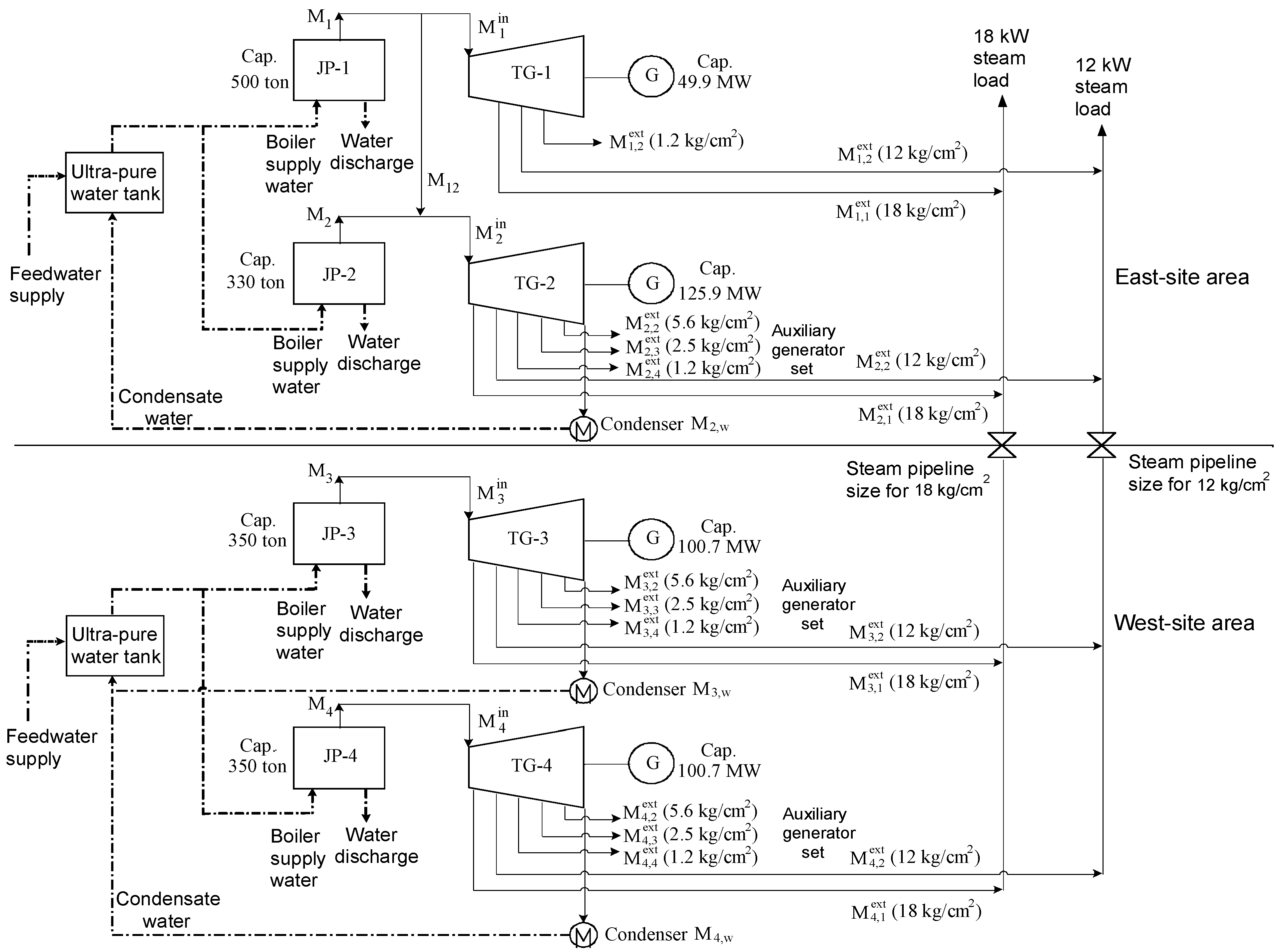
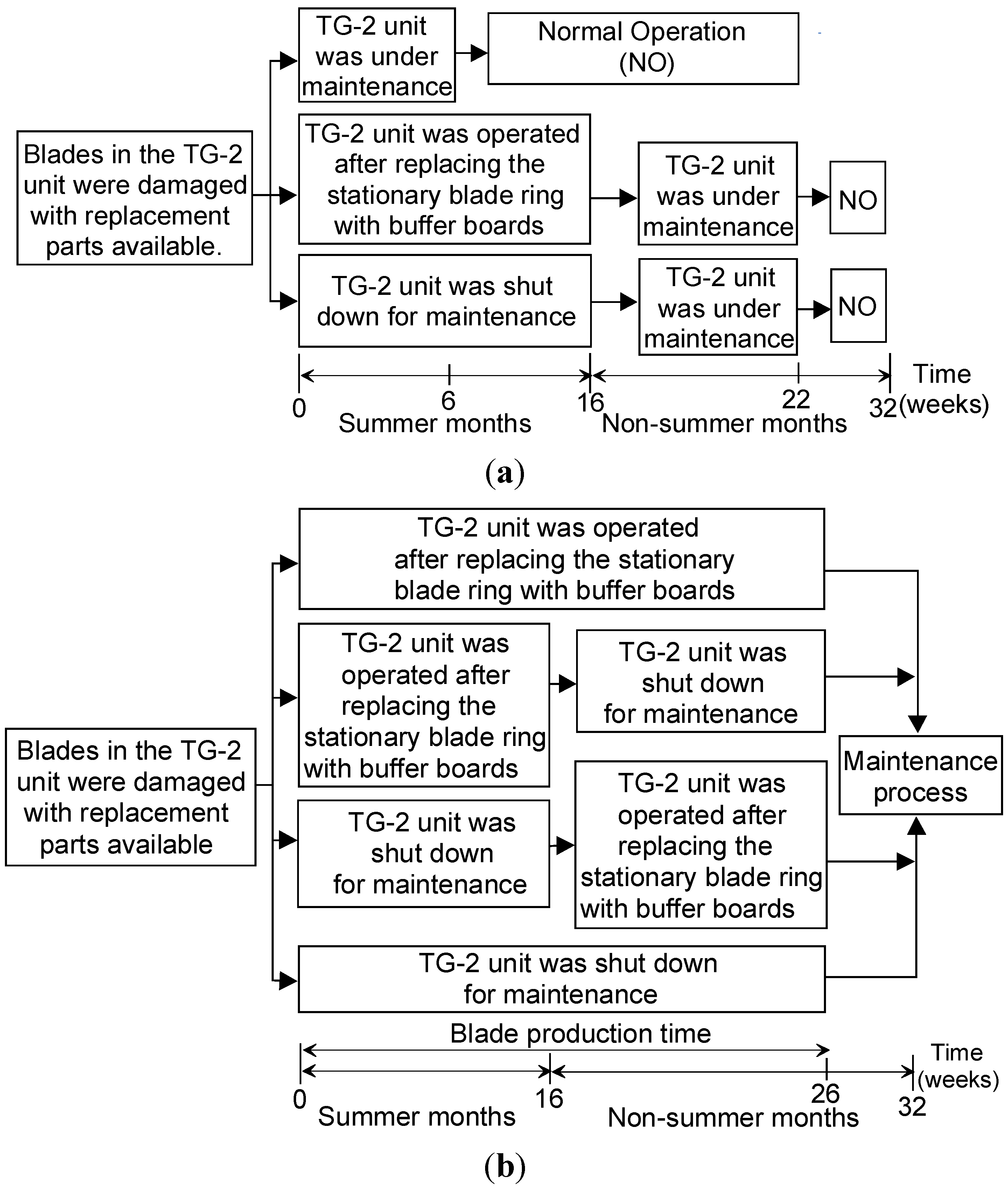
2. Strategic Decision-Making and Problem Formulation

The strategic decisions as shown in Figure 2 are based on whether replacement parts are readily available. This study investigates various scenarios consisting of shutting down the damaged TG-2 unit for maintenance and having continued operation of the TG-2 unit at a lower efficiency. Since the electricity rate varies based on the season (summer or non-summer) that the duration of maintenance periods may have a significant impact on the operating cost, this study will consider each 16-week period for summer and non-summer months. As can be seen from Figure 2, two different situations contain seven cases that are described in more detail below:

Situation 1: Replacement parts are readily available before the summer peak demand period. This situation has three cases:

Case Y1:

A complete inspection and overhaul of the TG-2 unit has been performed within six weeks and the unit continues to be operated normally for 22 weeks.

Case Y2:

The TG-2 unit has been operated for 16 weeks within summer electricity rate after an 80-h of replacing the stationary blade ring with buffer boards, and the unit resumes operation after carrying out a complete overhaul during non-summer months.

Case Y3:

The TG-2 unit has been shut down for maintenance during summer months, and the unit resumes operation after carrying out a complete overhaul during non-summer months.

Figure 2. Strategic paths under blade failures during the summer peak load periods for the studied plant. (a) With replacement parts available; (b) without replacement parts available.

Figure 2. Strategic paths under blade failures during the summer peak load periods for the studied plant. (a) With replacement parts available; (b) without replacement parts available.

Situation 2: Replacement parts are not readily available before the summer peak demand period. It will take 26 weeks to rebuild the blades and deliver to the site. This situation has four cases:

Case N1:

The TG-2 unit has been operated abnormally for 16 weeks within summer electricity rate and for 10 weeks within non-summer electricity rate after replacing the stationary blade ring with buffer boards. Then, a complete overhaul on the unit is performed.

Case N2:

The TG-2 unit has been operated abnormally for 16 weeks within summer electricity rate and has been shut down for 10 weeks of repairs during non-summer months. Then, a complete overhaul on the unit is performed.

Case N2:

The TG-2 unit has been shut down for maintenance during summer months and operated abnormally for 10 weeks within non-summer electricity rate after replacing the stationary blade ring with buffer boards. Then, a complete overhaul of the unit is performed.

Case N2:

The TG-2 unit has been shut down for maintenance during summer and non-summer months, and a complete overhaul of the unit is performed. This case assumes the TG-2 unit will return to a normal efficiency after the full overhaul.

As seen from Figure 1, the system has installed with one extraction back-pressure type and three extraction-condensing type steam turbines, spreading over two different locations 2-km apart. A two-pipe steam supply system at pressures of 18- and 12-kg/cm² with a maximum capacity of 110 tonnes/h is normally operated between the two locations. In the event of an emergency, the valves on the steam supply piping will automatically close. This study deals with the damage of blades in the TG-2 unit for the system caused economic issues that operations managers have to make strategic decisions. We will consider the time-of-use (TOU) rates, spinning reserves, relative operating limits and the cost of generating power in order to provide recommended decisions to operations managers in a time of the blade failure. In addition, other factors may be taken into consideration including:

(1)

I/O curve for each generating unit: To analyze the operating data and an isentropic effect of the steam boilers, it will help to determine the optimal operating points, the generating units’ efficiency characteristics and the performance of operational effectiveness.

(2)

Time-frame for the repair: Since the TOU rate varies by season, the cost of power consumption exceeding the contract capacity, due to a temporary failure, does vary. Moreover, the damaged unit operated at a lower efficiency may cause more fuel to be used, affecting the profits greatly.

(3)

The satisfaction of energy and steam needed in the manufacturing process: This factor takes into account ensuring that an adequate supply of steam and electricity is available to meet all manufacturing processes.

2.1. I/O Cost Curve Construction

The boiler I/O curve represents the relationship between the enthalpy of fuel consumed by the boiler and the steam produced by the boiler as shown in Table 1. It is used in energy saving evaluation. After performing regressions, a second-order polynomial provides a good fit to the data with R-squared as a measure of model validity. Thus, the boiler I/O cost curve is written as:

$$F_{i,t}=a_{i,0}+a_{i,1}\times M_{i,t}+a_{i,2}\times M_{i,t}^2$$

(1)

Then, the boiler I/O cost curve can be found by curve fitting techniques and the coefficients a_i,0–a_i,2 as shown in Table 2 can be found by using the least square minimization method according to the data as shown in Table 1. Similar to the boiler I/O cost curve, each turbine has its own I/O characteristic (i.e., the relationship between the enthalpy consumed and the electricity generated) to represent the unit’s efficiency. Normally, a higher efficiency turbine will exhaust steam with a lower enthalpy than a less efficiency turbine will do. The consumed enthalpy is obtained by subtracting the enthalpy of outlet steam from the enthalpy of inlet steam. The enthalpy of both inlet and outlet steam can be found from either the Mollier chart or the steam tables according to the pressure, temperature and flow rate of steam. Thus, the turbine’s I/O characteristic is written to be [12]:

$$P_{j,t}=b_{j,0}+{\displaystyle \sum _{k=1}^5{b}_{j,k}\times M_{j,k}^{\text{ext}}}\times \left(h_j^{\text{in}}-h_{j,k}^{\text{ext}}\right)+b_{j,6}\times M_{j,w}\times \left(h_j^{\text{in}}-h_{j,w}\right)$$

(2)

Note that the coefficients b_j,0–b_j,6 of the j-th turbines’ characteristic as shown in Table 3 are calculated by fitting a regression equation using Minitab which is a statics package developed by Pennsylvania State University (State College, PA, USA).

Table 1. Actual masses of coal utilized and steam produced for the four in-plant boilers.

Time (h)	JP-1		JP-2		JP-3		JP-4
	Mass of Steam Produced (tonne/h)	Mass of Coal Utilized (tonne/h)	Mass of Steam Produced (tonne/h)	Mass of Coal Utilized (tonne/h)	Mass of Steam Produced (tonne/h)	Mass of Coal Utilized (tonne/h)	Mass of Steam Produced (tonne/h)	Mass of Coal Utilized (tonne/h)
1	415	47.2	235	23.4	302	37.5	273.9	33
2	411.8	48	240	24	264.1	33.3	261.1	31
3	415.1	48	242	24.2	265.2	33.8	260	31
4	416.2	48.1	235	23.6	266.5	33.2	260.4	31
5	413.7	48.1	233	23	266.6	33.5	260.9	30.9
6	414	48	229	22.8	267.6	33.1	260.3	30.8
7	414.1	48	230	22.6	265.9	33.4	260.8	30.9
8	421.1	47.6	238	23.1	268.6	33.4	260.2	30.7
9	409.4	47.6	238	22.9	268	32.8	260.5	30.7
10	411	47.6	235	21.8	268.6	33.3	260.4	30.8
11	408.9	47.2	226	21.5	268.6	32.9	260	30.5
12	400.1	46.4	243	26.7	268.1	32.6	260.7	30.6
13	401.7	46.4	244	26.8	269	32.9	260.9	30.7
14	402.1	46.6	246	27	269	33.4	260.5	30.6
15	399	46.4	244	26.8	266.7	32.8	261.1	30.5
16	398	46.7	242	26.6	269.6	33.1	261.2	30.6
17	401	46.7	240	26.4	267.4	33.2	261.1	30.8
18	405	46.9	242	26.6	269.4	33.4	270.4	31.6
19	411	46.7	242	26.6	267.6	33.3	270.9	31.8
20	407	46.7	244	26.8	267.8	33.3	270.8	31.7
21	404	46.8	243	26.7	269	33.3	270.5	32
22	407.4	46.6	242	26.6	268	33.1	270.1	31.8
23	406.8	46.8	244	26.8	267	32.5	270.1	31.9
24	405.2	46.7	230	21.5	266.8	32.3	270.5	31.8

Table 1. Actual masses of coal utilized and steam produced for the four in-plant boilers.

Time (h)	JP-1		JP-2		JP-3		JP-4
	Mass of Steam Produced (tonne/h)	Mass of Coal Utilized (tonne/h)	Mass of Steam Produced (tonne/h)	Mass of Coal Utilized (tonne/h)	Mass of Steam Produced (tonne/h)	Mass of Coal Utilized (tonne/h)	Mass of Steam Produced (tonne/h)	Mass of Coal Utilized (tonne/h)
1	415	47.2	235	23.4	302	37.5	273.9	33
2	411.8	48	240	24	264.1	33.3	261.1	31
3	415.1	48	242	24.2	265.2	33.8	260	31
4	416.2	48.1	235	23.6	266.5	33.2	260.4	31
5	413.7	48.1	233	23	266.6	33.5	260.9	30.9
6	414	48	229	22.8	267.6	33.1	260.3	30.8
7	414.1	48	230	22.6	265.9	33.4	260.8	30.9
8	421.1	47.6	238	23.1	268.6	33.4	260.2	30.7
9	409.4	47.6	238	22.9	268	32.8	260.5	30.7
10	411	47.6	235	21.8	268.6	33.3	260.4	30.8
11	408.9	47.2	226	21.5	268.6	32.9	260	30.5
12	400.1	46.4	243	26.7	268.1	32.6	260.7	30.6
13	401.7	46.4	244	26.8	269	32.9	260.9	30.7
14	402.1	46.6	246	27	269	33.4	260.5	30.6
15	399	46.4	244	26.8	266.7	32.8	261.1	30.5
16	398	46.7	242	26.6	269.6	33.1	261.2	30.6
17	401	46.7	240	26.4	267.4	33.2	261.1	30.8
18	405	46.9	242	26.6	269.4	33.4	270.4	31.6
19	411	46.7	242	26.6	267.6	33.3	270.9	31.8
20	407	46.7	244	26.8	267.8	33.3	270.8	31.7
21	404	46.8	243	26.7	269	33.3	270.5	32
22	407.4	46.6	242	26.6	268	33.1	270.1	31.8
23	406.8	46.8	244	26.8	267	32.5	270.1	31.9
24	405.2	46.7	230	21.5	266.8	32.3	270.5	31.8

Table 2. Coefficients of I/O cost curve of the four in-plant boilers.

Boilers No.	Coefficients
	ai,0 (tonne/h)	ai,1 (dimensionless)	ai,2 (h/tonne)
JP-1	−10.30	0.1691	−0.000068
JP-2	−14.21	0.2291	−0.000250
JP-3	−38.53	0.3843	−0.000443
JP-4	56.00	−0.2871	0.000724

Table 2. Coefficients of I/O cost curve of the four in-plant boilers.

Boilers No.	Coefficients
	ai,0 (tonne/h)	ai,1 (dimensionless)	ai,2 (h/tonne)
JP-1	−10.30	0.1691	−0.000068
JP-2	−14.21	0.2291	−0.000250
JP-3	−38.53	0.3843	−0.000443
JP-4	56.00	−0.2871	0.000724

Table 3. Coefficients of steam turbines’ characteristic.

Generating units		Coefficients
		bj,0	bj,1	bj,2	bj,3	bj,4	bj,5	bj,6
TG-1		8.77	0.00062	0.00105	0.00072	0	0	0
TG-2	Abnormal	−12.80	0	−0.00097	0.00580	0.00222	0.02610	−0.00021
	Normal	−18.12	−0.0014	0.00145	0.00016	0.00294	0.00167	0.00152
TG-3		5.46	0	0.00009	0.00697	0.00111	0.01760	0.00004
TG-4		−2.44	0	0.00206	0.01060	0.00224	0.00282	0.00045

Table 3. Coefficients of steam turbines’ characteristic.

Generating units		Coefficients
		bj,0	bj,1	bj,2	bj,3	bj,4	bj,5	bj,6
TG-1		8.77	0.00062	0.00105	0.00072	0	0	0
TG-2	Abnormal	−12.80	0	−0.00097	0.00580	0.00222	0.02610	−0.00021
	Normal	−18.12	−0.0014	0.00145	0.00016	0.00294	0.00167	0.00152
TG-3		5.46	0	0.00009	0.00697	0.00111	0.01760	0.00004
TG-4		−2.44	0	0.00206	0.01060	0.00224	0.00282	0.00045

2.2. Mathematical Model

The optimal operation strategy takes into account the unit commitment and economic dispatch in an attempt to reduce cost, which is to raise the competitiveness of the cogeneration plant in the power market. The object function and relative constraints are discussed below.

2.2.1. Unit Commitment

The unit-commitment problem with the cogeneration system is to minimize the overall operation cost without affecting the reliability of steam and electricity supply while satisfying some constraints, such as the requirement of process steam and power demands. Since four generators have been installed at the plant, there will have a total of 2⁴ switch states at each time stage for a unit with a two-state representation (i.e., on or off). Thus, it may become more complex while taking into account practical unit-commitment schedules and operating constraints. The objective function of the unit commitment is to minimize the overall operation cost including the economic operation cost of each hour and the start-up cost of each unit.

$$\text{Objective} \text{function}: \text{Min }C={\displaystyle \sum _{t=1}^H{E}_t+{\displaystyle \sum _{t=1}^H{\displaystyle \sum _{i=1}^{N_{\text{b}}}S{T}_{i,t}}}}+{\displaystyle \sum _{t=1}^H{\displaystyle \sum _{j=1}^{N_{\text{tg}}}S{T}_{j,t}}}$$

(3)

2.2.2. Economic Operation Cost

The objective function of the economic operation cost, E, is defined as fuel cost of boilers, power interchange cost, make-up water cost and revenue of selling steam cost:

$$\text{Min }E={\displaystyle \sum _{i=1}^{N_{\text{b}}}\text{(}{F}_i\times F{C}_i\text{)}+P_{\text{tie}}}\times TOU+M_{\text{M}}\times W_{\text{p}}-\text{(}S{S}_{18}\times S_{\text{p},18}+S{S}_{12}\times S_{\text{p},12}\text{)}$$

(4)

where:

$$M_{\text{M}}=M_{18}+{\displaystyle \sum _{j=1}^4{M}_{j,12}}-Plan{t}_{18}-Plan{t}_{12}+{\displaystyle \sum _{i=1}^4{M}_i\times \frac{Blowdownrate}{1-Blowdownrate}}$$

(5)

$$S{S}_{18}=M_{18}-Plan{t}_{18}$$

(6)

$$S{S}_{12}={\displaystyle \sum _{j=1}^4{M}_{j,12}}-Plan{t}_{12}$$

(7)

Note that since steam driven auxiliary equipment in the plant and the condensing water at the condensing stage is treated as the circulating water with the assumption of a lossless pipe, the total consumption of water for operating the cogeneration plant is the sum of the steam extraction pressures of 18- and 12-kg/cm² as well as boiler blowdown water as shown in Equation (5). In addition, the blowdown water is about 3% of the boiler make-up water.

2.2.3. The Start-up Cost of Each Unit

The start-up cost consists mainly of the fuel cost, make-up water cost, labor cost and power consumption cost. Table 4 summarizes the start-up and incremental expenses of each unit for the studied plant. Note that if the start-up time of the TG-2/JP-2 unit in the system is over 8 h, the cost of start-up is estimated based on the cold start-up cost.

Table 4. Comparison of start-up costs between four generating units in the studied plant.

Start-up time (h)	Start-up costs (NT$)
	JP-1&TG-1	JP-2&TG-2	JP-3&TG-3	JP-4&TG-4
2	1,332,900	1,332,900	1,332,900	1,332,900
3	1,354,350	1,354,350	1,354,350	1,354,350
4	1,375,800	1,375,800	1,375,800	1,375,800
5	1,397,250	1,397,250	1,397,250	1,397,250
6	1,418,700	1,418,700	1,418,700	1,418,700
7	1,440,150	1,440,150	1,440,150	1,440,150
8	1,461,600	1,461,600	1,461,600	1,461,600
9	1,483,050	-	-	-

Table 4. Comparison of start-up costs between four generating units in the studied plant.

Start-up time (h)	Start-up costs (NT$)
	JP-1&TG-1	JP-2&TG-2	JP-3&TG-3	JP-4&TG-4
2	1,332,900	1,332,900	1,332,900	1,332,900
3	1,354,350	1,354,350	1,354,350	1,354,350
4	1,375,800	1,375,800	1,375,800	1,375,800
5	1,397,250	1,397,250	1,397,250	1,397,250
6	1,418,700	1,418,700	1,418,700	1,418,700
7	1,440,150	1,440,150	1,440,150	1,440,150
8	1,461,600	1,461,600	1,461,600	1,461,600
9	1,483,050	-	-	-

2.2.4. Equality and Inequality Constraints

(a)

Power balance:

$$P_{\text{tie},t}={\displaystyle \sum _{j=1}^{N_{\text{tg}}}{U}_{j,t}\times P_{j,t}-P_{\text{D},t}}$$

(8)

(b)

Generation capacity limits (as shown in Table 5):

$$P_{j,\text{ min}}\le P_{j,t}\le P_{j, \text{max}} \text{for} j=1,2,3,4$$

(9)

$$M_{i,\min }\le M_{i.t}\le M_{i,\text{max}}\text{ for }j=1,2,3,4$$

(10)

$$M_{j,18,\text{min}}\le M_{j,18}\le M_{j,18,\text{max}}\text{ for }j=1,2,3,4$$

(11)

$$M_{j,12,\text{min}}\le M_{j,12}\le M_{j,12,\text{max}}\text{ for }j=1,2,3,4$$

(12)

$$M_{j,\text{p2},\text{min}}\le M_{j,\text{p2}}\le M_{j,\text{p2,max}}\text{ for }j=2,3,4$$

(13)

$$M_{j,\text{p3,min}}\le M_{j,\text{p3}}\le M_{j,\text{p3,max}}\text{ for }j=2,3,4$$

(14)

$$M_{j,\text{p4,min}}\le M_{j,\text{p4}}\le M_{j,\text{p4},\text{max}} \text{for} j=2,3,4$$

(15)

$$M_{j,\text{W,min}}\le M_{j,\text{W}}\le M_{j,\text{W,max}}\text{ for }j=2,3,4$$

(16)

Note that M_j,p2, M_j,p3 and M_j,p4 are the extraction steam used to heat the auxiliary with no control, but instead of having the valve to open to a certain point.

Table 5. Upper and lower limits of in-plant boilers and steam turbines.

Unit No.	Steam input source	Electricity output of each generator (MW)		Boilers No.	Boiler steam production (tonne/h)
		Pj,min	Pj,max		Mi,min	Mi,max
TG-1	JP-1	10	49.9	JP-1	170	500
TG-2	JP-1, JP-2	10	125.9	JP-2	110	330
TG-3	JP-3	22	100.7	JP-3	150	350
TG-4	JP-4	22	100.7	JP-4	150	350

Table 5. Upper and lower limits of in-plant boilers and steam turbines.

Unit No.	Steam input source	Electricity output of each generator (MW)		Boilers No.	Boiler steam production (tonne/h)
		Pj,min	Pj,max		Mi,min	Mi,max
TG-1	JP-1	10	49.9	JP-1	170	500
TG-2	JP-1, JP-2	10	125.9	JP-2	110	330
TG-3	JP-3	22	100.7	JP-3	150	350
TG-4	JP-4	22	100.7	JP-4	150	350

(c)

Flow conservation constraints:

$$M_1^{\text{in}}=M_1-M_{12}$$

(17)

$$M_2^{\text{in}}=M_2+M_{12}$$

(18)

$$M_3^{\text{in}}=M_3$$

(19)

$$M_4^{\text{in}}=M_4$$

(20)

(d)

Steam flow capacity constraints of the j-th turbine:

$$M_1^{\text{in}}=M_{1,18}+M_{1,12}+M_{1,\text{ p2}}$$

(21)

$$M_j^{\text{in}}=M_{j,18}+M_{j,12}+M_{j,\text{ p2}}+M_{j,\text{ p3}}+M_{j,\text{ p4}}+M_{j,\text{ W}},\text{ for }j=2,3,4$$

(22)

(e)

Steam balance:

$${\displaystyle \sum _{j=1}^{N_{\text{tg}}}{M}_{j,\text{ 18}}}\ge S{S}_{t,18}+Plan{t}_{t,18}$$

(23)

$${\displaystyle \sum _{j=1}^{N_{\text{tg}}}{M}_{j,\text{ 12}}}\ge S{S}_{t,12}+Plan{t}_{t,12}$$

(24)

(f)

Capacity limit of steam connecting pipe:

$$M_{3,\text{ 18}}+M_{4,18}\le C{H}_{18,\text{ max}}$$

(25)

$$M_{3,\text{ 12}}+M_{4,12}\le C{H}_{12,\text{ max}}$$

(26)

(g)

Spinning reserve:

$${\displaystyle \sum _{j=1}^{N_{\text{tg}}}\text{(}{U}_{j,t}}{P}_{j,\text{ max}}-P_{\text{D},t}\text{)}\ge 20\%\times P_{\text{D},t}$$

(27)

Because of the small contracted power and huge penalty of overtaking the contracted power by Taiwan Power Company (TPC), the emergency load shedding program in a cogeneration plant will be activated to avoid overtaking contracted power when some generation units are tripped. The spinning reserve in this paper is defined as 20% of the electric demand, which means that the total output power of on-line units minus the electric demand should be more than 20% of the electric demand, to avoid overtaking contracted power from TPC.

(h)

Minimum up-time/down-time limit of units:

$$T_{j,\text{ on}}\ge MU{T}_j$$

(28)

$$T_{j,\text{ off}}\ge MD{T}_j$$

(29)

$$T_{i,\text{ on}}\ge MU{T}_i$$

(30)

$$T_{i,\text{ off}}\ge MD{T}_i$$

(31)

The minimum up- and down-time constraints of the boiler/steam turbine system in the studied plant are listed in Table 6. Both constraints are used to ensure the safety running of units. For the studied plant, the state of a generating unit is called hot start if the unit is starting up within 8 h after it has been shut down. The state of a generating unit is called warm start if the unit is starting up between 9 and 32 h after it has been shut down. The state of a generating unit is called cold start if the unit is starting up after it has been shut down more than 32 h.

Table 6. Minimum up- and down-time constraints of the boiler/steam turbine system.

Boile/Turbine	Hot start (h)	Warm start (h)	Cold start (h)	Low load/Shutdown (h)
P-1/TG-1	2/1	5/1	9/2	3/1
JP-2/TG-2	2/1	4/1	8/2	3/1
JP-3/TG-3	2/1	4/1	8/2	3/1
JP-4/TG-4	2/1	4/1	8/2	3/1

Table 6. Minimum up- and down-time constraints of the boiler/steam turbine system.

Boile/Turbine	Hot start (h)	Warm start (h)	Cold start (h)	Low load/Shutdown (h)
P-1/TG-1	2/1	5/1	9/2	3/1
JP-2/TG-2	2/1	4/1	8/2	3/1
JP-3/TG-3	2/1	4/1	8/2	3/1
JP-4/TG-4	2/1	4/1	8/2	3/1

3. Simulation Results

3.1. Case Description

The simulated cases are analyzed based on the aforementioned objective functions for the unit commitment and economic dispatch to meet the specific constraints of the studied plant. If the turbine’s efficiency is less than 50%, it will cost twice as much to produce electricity from the public utility as it does to produce electricity from the system. However, the turbine’s efficiency was around 78% after removing the low-pressure blades of the TG-2 unit and replacing the stationary blade ring with buffer boards. Thus, this study will focus on analyzing the strategy of operating a generator under blades failure for the cases if replacement parts are readily available and replacement parts are not readily available.

For this study, we have assumed the TG-2 unit will return back to a normal efficiency after the full overhauling. In addition, the electricity demand and steam requirement for each week are assumed to be periodically observed. The simulated times for summer and non-summer months are from 28 July to 4 August and from 26 October to 2 November, respectively. Thus, the total of simulated hours for all cases are 168 h. All relevant data used in this study are as follows:

(1)

The capacity price with contracts signed in 2006 is listed in Table 7.

(2)

The time-of-use rates announced by the utility on August 2006 are listed in Table 8 and Table 9.

(3)

The assumed coal purchase price and fuel oil price are 2.004 NT$/kg and 12.9 NT$/L, respectively.

(4)

The operating cost of boiler make-up water is 30 NT$/tonne and the boiler blowdown rate is 3%.

(5)

The sale prices of the steam pressures at 18 and 12 kg/cm² are assumed to be 471 and 424 NT$/tonne, respectively.

(6)

The coal/steam ratio of JP-1, JP-2, JP-3 and JP-4 boilers are equal to the mass (in tonne/h) of coal utilized divided by the mass (tonne/h) of steam produced which are 116.050, 99.414, 120.131 and 116.409, respectively.

Table 7. Contract capacity rate signed by August 2006.

Items		Summer peak	Summer off-peak
Basic electricity price (NT$)	Annual contract	217.3	160.6
	Semi-peak contract	160.6	160.6
	Saturday semi-peak and off-peak contract	43.4	32.1

Table 7. Contract capacity rate signed by August 2006.

Items		Summer peak	Summer off-peak
Basic electricity price (NT$)	Annual contract	217.3	160.6
	Semi-peak contract	160.6	160.6
	Saturday semi-peak and off-peak contract	43.4	32.1

Table 8. Rate of purchasing electricity from the utility. TOU: time-of-use.

Items			TOU rate (NT$/kW·h)
			Summer months	Non-summer months
Weekday	On-peak	10:00–12:00	3.29	-
		13:00–17:00
	Semi-peak	07:30–10:00	1.9	-
		12:00–13:00
		17:00–22:30
		07:30–22:30	-	1.85
	Off-peak	00:00–07:30	0.78	0.73
		22:30–24:00
Saturday	Semi-peak	07:30–22:30	1.08	1.02
	Off-peak	All day	0.78	0.73
Sunday	Off-peak	All day	0.78	0.73

Note: The summer months are June through September. The non-summer months are January through May and October through December.

Table 8. Rate of purchasing electricity from the utility. TOU: time-of-use.

Items			TOU rate (NT$/kW·h)
			Summer months	Non-summer months
Weekday	On-peak	10:00–12:00	3.29	-
		13:00–17:00
	Semi-peak	07:30–10:00	1.9	-
		12:00–13:00
		17:00–22:30
		07:30–22:30	-	1.85
	Off-peak	00:00–07:30	0.78	0.73
		22:30–24:00
Saturday	Semi-peak	07:30–22:30	1.08	1.02
	Off-peak	All day	0.78	0.73
Sunday	Off-peak	All day	0.78	0.73

Note: The summer months are June through September. The non-summer months are January through May and October through December.

Table 9. Rate of selling electricity back to the utility. Unit: NT$.

Items			Within the 20% installed capacity		Over the 20% installed capacity
			Summer peak	Summer off-peak	Summer peak	Summer off-peak
Basic electricity price		Per kW	207	153	202.86	149.94
TOU rate	On-peak	Per kW·h	3.04	-	3.0237	-
	Semi-peak	Per kW·h	1.83	1.77	1.6432	1.5861
	Saturday semi-peak	Per kW·h	1.00	0.94	0.8142	0.757
	Off-peak	Per kW·h	0.69	0.64	0.5194	0.471

Table 9. Rate of selling electricity back to the utility. Unit: NT$.

Items			Within the 20% installed capacity		Over the 20% installed capacity
			Summer peak	Summer off-peak	Summer peak	Summer off-peak
Basic electricity price		Per kW	207	153	202.86	149.94
TOU rate	On-peak	Per kW·h	3.04	-	3.0237	-
	Semi-peak	Per kW·h	1.83	1.77	1.6432	1.5861
	Saturday semi-peak	Per kW·h	1.00	0.94	0.8142	0.757
	Off-peak	Per kW·h	0.69	0.64	0.5194	0.471

3.2. Considering the Time-of-Use Rate into Decision-Making

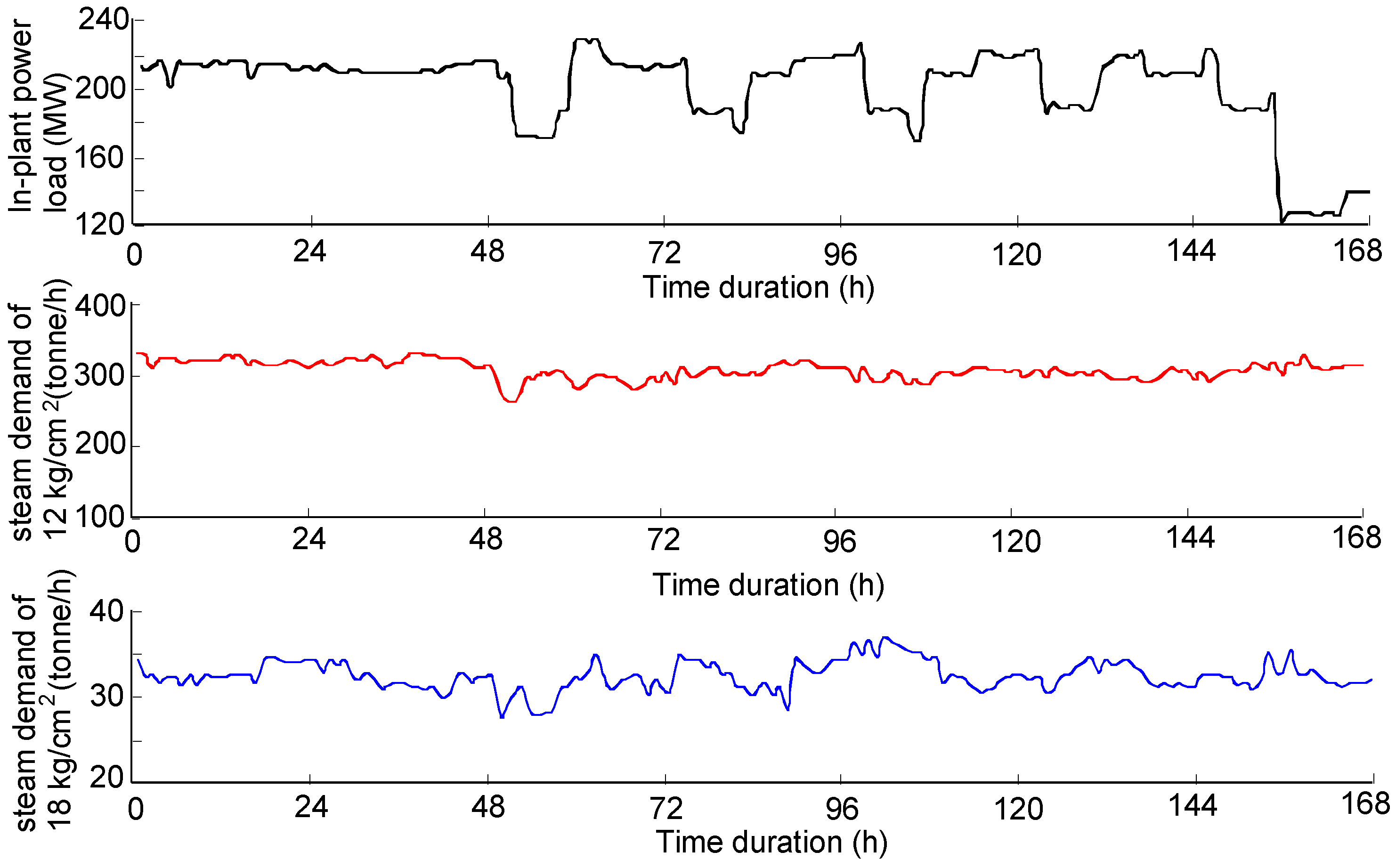
3.2.1. During the Summer Months

Since the steam requirement and electricity demand were consistent throughout the week, they were used only for one week to assess the operational costs under three different situations during the summer months. Figure 3 shows the curves of in-plant power load and steam demand for one week during the summer months. For Cases Y1, Y2 and Y3, we assumed that the steam demand, in-plant power load and I/O curves of the boilers and turbines (except the TG-2 unit) are the same in each case. The simulation results show that shifting 10% of in-plant electric loads to off-peak rate periods can make profits when the steam consumption in the plant during the summer months remains practically unchanged. The total costs over a period of 168 h for Cases Y1, Y2 and Y3 are 12,254,394 NT$, 14,379,317 NT$ and 20,308,900 NT$, respectively, when considering the unit commitment and economic dispatch. Thus, the operating cost of running the plant for Case Y2 is about 2,124,923 NT$, which is higher than that of Case Y1. On the other hand, there is an increase of about 5,929,583 NT$ in operating cost of running the plant for Case Y3 as compared to Case Y2. This is due to the difference of the coal/steam ratio among boilers. When the TG-2 unit is shut down for maintenance, the JP-2 boiler has to be shut down. Thus, units with a lower coal/steam ratio are needed to share in steam production, resulting in a cost increase of fuel.

Figure 3. In-plant power load and steam demands during the summer months.

Figure 3. In-plant power load and steam demands during the summer months.

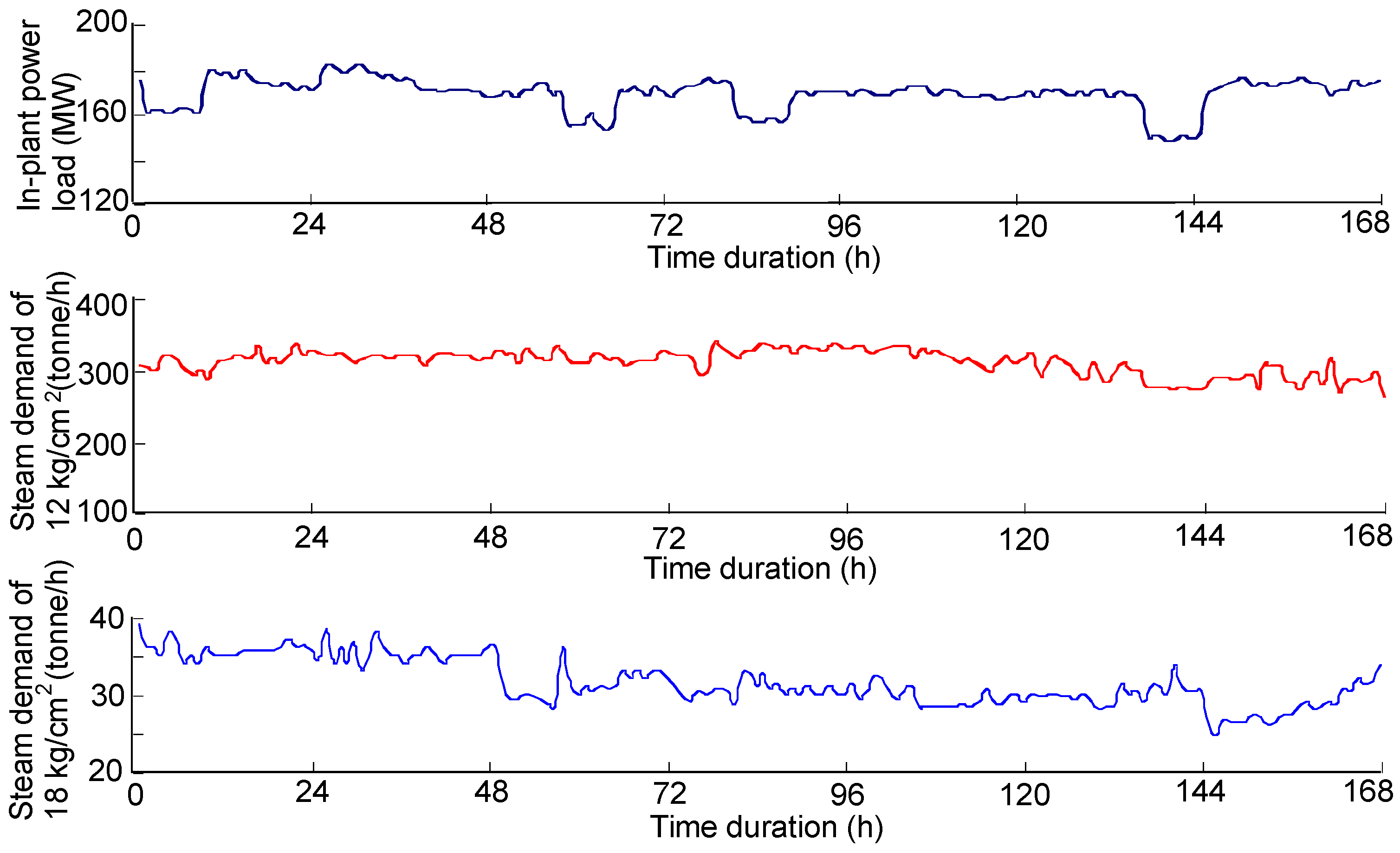
3.2.2. During the Non-Summer Months

To prevent initiating a chain reaction of units to use backup power, operations managers had decided to install a new blade when the electricity demand was low in the middle of December. In between times, a record of abnormal operating conditions on the TG-2 unit had practically occurred during the non-summer months. The TOU rate in the non-summer months was four months for the same three scenarios aforementioned above for the purpose of comparison, and the curves of in-plant power load and steam demand for one week during the non-summer months are shown in Figure 4. The total costs over a period of 168 h for Cases Y1, Y2 and Y3 are 13,771,791 NT$, 15,119,318 NT$ and 19,121,263 NT$, respectively, when considering the unit commitment and economic dispatch. The operating cost of running the plant for Case Y3 is greater than that of Case Y2. This is mainly due to the difference of the coal/steam ratio among boilers and no fair-tariff guarantee for cogenerated electricity. In addition, demands for electricity and process steam, as well as spinning reserve, for the studied plant can be satisfied by other units under normal operating conditions if the TG-2 unit is shutdown for repair work during the non-summer months. However, there may be a penalty charge for exceeding the contract capacity and lead to a decrease in the profit of selling electricity if a fault has occurred during the non-summer months.

Figure 4. In-plant power load and steam demands during the non-summer months.

Figure 4. In-plant power load and steam demands during the non-summer months.

A comparison of total costs for Cases Y1, Y2 and Y3 is listed in Table 10. As seen from Table 10, the total cost of operating the TG-2 unit under abnormal conditions for the TOU rates in both the summer and non-summer months is less than the actual cost. Furthermore, the TG-2 unit under shutdown maintenance over a 168-h period in both the summer and non-summer months will cost 5,005,700 NT$ and 3,324,640 NT$ more, respectively, compared to the actual cost. This is because the JP-2 boiler has the highest coal/steam ratio among boilers. When the TG-2 unit is shut down for maintenance, the JP-2 boiler has to be shut down. Thus, units with a lower coal/steam ratio are needed to share in steam production, resulting in a cost increase of fuel.

Table 10. Comparison of total costs under different operating conditions.

TOU rates	Operating conditions of the TG-2 turbine	Total costs (NT$/week)
Summer months	Actual recording	15,303,200
	Case Y1	12,254,394
	Case Y2	14,379,317
	Case Y3	20,308,900
Non-summer months	Actual recording	15,796,623
	Case Y1	13,771,791
	Case Y2	15,119,318
	Case Y3	19,121,263

Table 10. Comparison of total costs under different operating conditions.

TOU rates	Operating conditions of the TG-2 turbine	Total costs (NT$/week)
Summer months	Actual recording	15,303,200
	Case Y1	12,254,394
	Case Y2	14,379,317
	Case Y3	20,308,900
Non-summer months	Actual recording	15,796,623
	Case Y1	13,771,791
	Case Y2	15,119,318
	Case Y3	19,121,263

3.3. Maintenance Strategies Decision Making

We will use the expected value as a risk index to evaluate whether the TG-2 unit should be shut down immediately for maintenance in the summer months, and to estimate the risk cost of facing the loss of the TG-2 unit for specified duration. The risk index is the product of a probability of failure occurrence and potential consequence of failure. According to statistics provided by the cogeneration plant, a generating unit can be put back in service within 24 h if it is out of service, and in most cases repairs are completed within three days if a boiler pipe cracks. In addition, we have assumed operating a unit under abnormal conditions is an independent event, since two units have never encountered abnormal operations simultaneously. The probability of any unusual or abnormal conditions of boilers and steam turbines observed in the plant during each of the past four years (i.e., 2004–2007) is tabulated in Table 11. The probability as listed in Table 11 is obtained by dividing the total hours of abnormal conditions by the actual operating hours.

Table 11. Probability of the four in-plant boilers and steam turbines during the past four years.

Items	Unit 1				Unit 2				Unit 3				Unit 4
	Years				Years				Years				Years
	2004	2005	2006	2007	2004	2005	2006	2007	2004	2005	2006	2007	2004	2005	2006	2007
Number of abnormal situations	0	0	0	1	1	2	3	2	1	2	3	3	1	2	3	1
Total shutdown hour (h)	0	0	0	4	3	8	166	35	37	42	26	23	3	8	16.5	4
Actual operating hours (h)	8,760				34,080				34,080				34,080
Probability of occurring faults	0.0457%				0.6221%				0.3756%				0.0924%

Table 11. Probability of the four in-plant boilers and steam turbines during the past four years.

Items	Unit 1				Unit 2				Unit 3				Unit 4
	Years				Years				Years				Years
	2004	2005	2006	2007	2004	2005	2006	2007	2004	2005	2006	2007	2004	2005	2006	2007
Number of abnormal situations	0	0	0	1	1	2	3	2	1	2	3	3	1	2	3	1
Total shutdown hour (h)	0	0	0	4	3	8	166	35	37	42	26	23	3	8	16.5	4
Actual operating hours (h)	8,760				34,080				34,080				34,080
Probability of occurring faults	0.0457%				0.6221%				0.3756%				0.0924%

Let’s assume the TG-2 unit is shut down for maintenance and the rest of the three units are operated continuously. If the most serious damage occurred in the piping system of a steam boiler and resulted in shutting down the turbine without affecting other units, the system can still produce enough steam to meet the manufacturing needs, but it may cause the supply electricity to drop sharply, resulting in purchasing power from the grid instead of selling electricity. Thus, we will discuss about charges for exceeding the contract demand, loss of profits during the maintenance period, and restart costs after maintenance under consideration given the power load shortage. The loss of profits will depend on the time-of-use rates and the capacity of exceeding the contract power. The aforementioned costs can be found according to a formula and descriptions provided by the cogeneration plant as below:

(a)

The penal charges for exceeding the contract demand, C_P: it is written to be 2 × (the maximum exceeded power consumption is less than 10% of the contract demand × basic tariff) + 3 × (the maximum exceeded power consumption is more than 10% of the contract demand × basic tariff).

(b)

The loss of profits, C_L: It means the cost of purchasing energy from the utility instead of selling that energy during the maintenance period, which is calculated by multiplying the purchase price of energy by the TOU rate.

(c)

The restart cost, C_S: It can be obtained based on calculating the cold start-up cost.

Therefore, when a boiler/turbine set is being shut down, the total expected losses can be obtained by multiplying the total losses by the probability of fault risk factor. Table 12 lists a comparison of the operational costs and expected losses of difference cases for one week. As seen from Table 12, the expected loss of a generating unit during the summer months is higher than that of the non-summer months. This is mainly caused by the TOU rate and spinning reserve tariff. Thus, the total expected loss for operating the TG-2 unit under normal conditions is larger than the one under abnormal conditions since the probability of a fault occurring in the Unit 2 is larger than the others.

Table 12. Comparison of the operational costs and expected losses of different cases. Unit: NT$/week.

Items	TOU rate during summer months			TOU rate during non-summer months
	Shutdown maintenance	Abnormal operation	Normal operation	Shutdown maintenance	Abnormal operation	Normal operation
Operational cost	20,308,900	14,379,317	12,254,394	19,121,263	15,119,319	13,771,791
Expected loss of unit 1	328,967	78,586	93,028	88,257	68,149	90,308
Expected loss of unit 2	0	3,428,981	5,021,015	0	1,263,816	4,348,737
Expected loss of unit 3	13,783,512	4,623,253	4,212,521	13,112,259	3,929,824	2,775,196
Expected loss of unit 4	2,766,203	886,020	838,635	884,982	954,645	513,873
Total expected loss	16,878,682	9,016,840	10,165,198	14,085,498	6,216,433	7,728,114

Table 12. Comparison of the operational costs and expected losses of different cases. Unit: NT$/week.

Items	TOU rate during summer months			TOU rate during non-summer months
	Shutdown maintenance	Abnormal operation	Normal operation	Shutdown maintenance	Abnormal operation	Normal operation
Operational cost	20,308,900	14,379,317	12,254,394	19,121,263	15,119,319	13,771,791
Expected loss of unit 1	328,967	78,586	93,028	88,257	68,149	90,308
Expected loss of unit 2	0	3,428,981	5,021,015	0	1,263,816	4,348,737
Expected loss of unit 3	13,783,512	4,623,253	4,212,521	13,112,259	3,929,824	2,775,196
Expected loss of unit 4	2,766,203	886,020	838,635	884,982	954,645	513,873
Total expected loss	16,878,682	9,016,840	10,165,198	14,085,498	6,216,433	7,728,114

3.3.1. Replacement Blades Are Readily Available

This subsection discusses the strategy of making decisions on either immediately shutting down the abnormal unit for maintenance during the summer months or postponing maintenance until the non-summer months when replacement blades are readily available. Table 13 lists the average operating costs and expected losses of simulated cases in terms of NT$ per hour. As seen from Table 13, shutting the turbine down immediately to replace the blades is the best strategy. Its operating cost is NT$ 166,414 per hour.

Table 13. Total costs of operating the TG-2 steam turbine when there are replacement blades. Unit: NT$/h.

Items	During summer months					During non-summer months
	With Extra Blades			Without Extra Blades		With Extra Blades	Without Extra Blades
	Shutdown maintenance	Abnormal operation	Shutdown without maintenance	Abnormal operation	Shutdown without maintenance	Shutdown maintenance	Shutdown maintenance	Abnormal operation
Average operating cost	90,922	85,591	120,886	85,591	120,886	93,916	113,817	98,929
Expected loss	75,493	53,672	100,468	53,672	100,468	60,191	83,842	54,567
Abnormal operating cost	0	80,000	0	80,000	0	0	0	0
Total costs	166,414	219,263	221,355	219,263	221,355	154,107	197,659	153,496

Table 13. Total costs of operating the TG-2 steam turbine when there are replacement blades. Unit: NT$/h.

Items	During summer months					During non-summer months
	With Extra Blades			Without Extra Blades		With Extra Blades	Without Extra Blades
	Shutdown maintenance	Abnormal operation	Shutdown without maintenance	Abnormal operation	Shutdown without maintenance	Shutdown maintenance	Shutdown maintenance	Abnormal operation
Average operating cost	90,922	85,591	120,886	85,591	120,886	93,916	113,817	98,929
Expected loss	75,493	53,672	100,468	53,672	100,468	60,191	83,842	54,567
Abnormal operating cost	0	80,000	0	80,000	0	0	0	0
Total costs	166,414	219,263	221,355	219,263	221,355	154,107	197,659	153,496

3.3.2. Replacement Blades Are Not Readily Available

This subsection presents a practical situation analysis that replacement blades are not readily available. For purchase of remanufactured turbine blades, it may take 26 weeks for delivery. Before being replaced with the new blades, the TG-2 unit is either shut down for maintenance or is operated under abnormal conditions. Table 13 lists the average operating costs and expected losses of simulated cases in terms of NT$ per hour. As seen from Table 13, operating the system in abnormal conditions before the new blades delivered is the best strategy. Its operating cost is NT$ 219,263 per hour.

4. Results and Discussion

This section summarizes some major findings and recommendations of the aforementioned cases. The decision suggestion concluded here may be still applicable, even though turbines may have different degrees of blade damage, reduce its efficiency and occur faults at different times. After the cogeneration plant began commercial operation in 2007, only the TG-2 unit has not yet been installed, after more than 15 years it still has a fair-tariff guarantee. If the TG-2 unit is shut down for maintenance in the summer months, it may increase the risk of violation of the contract capacity. Thus, operation managers had decided to operate the TG-2 unit continuously under abnormal conditions that may maximize profits.

Before shutting the damaged turbine down for maintenance or beginning to remove the low-pressure blades of the TG-2 steam turbine and replace the stationary blade ring with buffer boards for restoration service, it is important to consider the level of efficiency decrease in the generating unit, the difference between TOU rates and regular rates, risks, profits and processing fees. According to abnormal data obtained from the plant, the TG-2 unit has the highest failure rate. Thus, regularly scheduled maintenance can increase the efficiency of the steam turbine and reduce risk and costs, resulting in increasing maintenance costs.

In addition, operations managers can strategically use TOU rates to dispatch the turbines since the TOU rates during summer on- and off-peak hours may have an economic impact of the cogeneration operation. Thus, profits can be maximized if the load is transferred from on-peak to semi- and off-peak hours. Furthermore, before shutting down the damaged unit for maintenance, if the unit is operated under abnormal conditions such that the efficiency has decreased significantly, operations managers should consider the degree of efficiency drop, the TOU rate, risks (e.g., spinning-reserve penalties, power consumption over the contract capacity, failure rate, etc.) and profits. Thus, this will result in greater losses if the damaged unit is shut down for maintenance in the summer months.

Lastly, although the TG-2 unit has the best coal/steam ratio among all units, the total operating cost and expected loss (or risk cost) to shut it down for maintenance during the non-summer months are 252,445,489 NT$ and 161,794,133 NT$, respectively. Thus, the overall expense of having continued operation of the plant during the non-summer months is 414,239,622 NT$. However, the total operating cost and expected loss to shut it down for maintenance during the summer months are 244,397,33 NT$ and 202,924,072 NT$, respectively. Thus, the overall expense of having continued operation of the plant during the summer months is 447,321,409 NT$.

5. Conclusions

This paper presents experiences from dealing with practical issues related to the operation of steam turbines under blade failures during the summer peak load periods at a cogeneration plant in Taiwan. To ensure the continuity of electricity supply and minimize total profit losses, operations managers have to make effective decisions whether the generating unit experienced turbine blade failures should be shut down for maintenance immediately rather than have continued operation or vice versa. Based on the simulation results, we have recommended that the TG-2 unit should continue operating after removing the low-pressure blades and replacing the stationary blade ring with buffer boards, because it is economically better than shutting down the TG-2 unit for maintenance. This is in agreement with the critical decisions made at the time of a blade failure. Hopefully, the findings of this study may provide suggestions for other cogeneration plants that encounter abnormal operating conditions.

References

1. Li, T.; Shahidehpour, M. Price based unit commitment: A case of Lagrangian relaxation versus mixed integer programming. IEEE Trans. Power Syst. 2005, 20, 2015–2025. [Google Scholar] [CrossRef]
2. Senjyo, T.; Shimabukuro, K.; Uezato, K.; Funabashi, T. A fast technique for unit commitment problem by extended priority list. IEEE Trans. Power Syst. 2003, 18, 882–888. [Google Scholar] [CrossRef]
3. Venkatesh, B.N.; Chankong, V. Decision models for management of cogeneration plants. IEEE Trans. Power Syst. 1995, 10, 1250–1256. [Google Scholar] [CrossRef]
4. Ashok, S.; Banerjee, R. Optimal operation of industrial cogeneration for load management. IEEE Trans. Power Syst. 2003, 18, 931–937. [Google Scholar] [CrossRef]
5. Casolino, G.M.; Losi, A.; Russo, C. Design choices for combined cycle units and profit-based unit commitment. Int. J. Electr. Power Energy Syst. 2012, 42, 693–700. [Google Scholar]
6. Basu, M. Artifical immune system for combined heat and power economic dispatch. Int. J. Electr. Power Energy Syst. 2012, 43, 1–5. [Google Scholar] [CrossRef]
7. Basu, M. Combined heat and power economic emission dispatch using nondominated sorting genetic algorithm-II. Int. J. Electr. Power Energy Syst. 2013, 53, 135–141. [Google Scholar] [CrossRef]
8. Peik-Herfeh, M.; Seifi, H.; Sheikh-El-Eslami, M.K. Decision making of a virtual power plant under uncertainties for bidding in a day-ahead market using point estimate method. Int. J. Electr. Power Energy Syst. 2013, 44, 88–98. [Google Scholar] [CrossRef]
9. Kazarlis, S.A.; Bakirtizis, A.G.; Petridis, V. A genetic algorithm solution to the unit commitment problem. IEEE Trans. Power Syst. 1996, 11, 83–92. [Google Scholar] [CrossRef]
10. Swarup, K.S.; Yamashiro, S. Unit commitment solution methodology using genetic algorithm. IEEE Trans. Power Syst. 2002, 17, 87–91. [Google Scholar] [CrossRef]
11. Lu, B.; Shahidehpour, M. Unit commitment with flexible generating units. IEEE Trans. Power Syst. 2005, 20, 1022–1034. [Google Scholar] [CrossRef]
12. Duff, M.C.; Price, W.G., Jr.; Davis, A.N.; Manuel, E.H., Jr. Cogen3: A Computer Model for Design, Costing, and Economic Operation of Cogeneration Projects; EPRI-EA-3995; EPRI (Electric Power Research Institute): Palo Alto, CA, USA, 1985. [Google Scholar]