Preliminary Design and Simulation of a Turbo Expander for Small Rated Power Organic Rankine Cycle (ORC)

Abstract

Nowadays, the Organic Rankine Cycle (ORC) system, which operates with organic fluids, is one of the leading technologies for “waste energy recovery”. It works as a conventional Rankine Cycle but, as mentioned, instead of steam/water, an organic fluid is used. This change allows it to convert low temperature heat into electric energy where required. Large numbers of studies have been carried out to identify the most suitable fluids, system parameters and the various configurations. In the present market, most ORC systems are designed and manufactured for the recovery of thermal energy from various sources operating at “large power rating” (exhaust gas turbines, internal combustion engines, geothermal sources, large melting furnaces, biomass, solar, etc.); from which it is possible to produce a large amount of electric energy (30 kW ÷ 300 kW). Such applications for small nominal power sources, as well as the exhaust gases of internal combustion engines (car sedan or town, ships, etc.) or small heat exchangers, are very limited. The few systems that have been designed and built for small scale applications, have, on the other hand, different types of expander (screw, scroll, etc.). These devices are not adapted for placement in small and restricted places like the interior of a conventional car. The aim of this work is to perform the preliminary design of a turbo-expander that meets diverse system requirements such as low pressure, small size and low mass flow rates. The expander must be adaptable to a small ORC system utilizing gas of a diesel engine or small gas turbine as thermal source to produce 2–10 kW of electricity. The temperature and pressure of the exhaust gases, in this case study (400–600 °C and a pressure of 2 bar), imposes a limit on the use of an organic fluid and on the net power that can be produced. In addition to water, fluids such as CO₂, R134a and R245fa have been considered. Once the operating fluids has been chosen, the turbine characteristics (dimensions, input and output temperature, pressure ratio, etc.) have been calculated and an attempt to find the “nearly-optimal” combination has been carried out. The detailed design of a radial expander is presented and discussed. A thermo-mechanical performance study was carry out to verify structural tension and possible displacement. On the other hand, preliminary CFD analyses have been performed to verify the effectiveness of the design procedure.

1. Introduction

The Organic Rankine Cycle (ORC) converts thermal energy into mechanical shaft power. The benefit of ORC systems is the recovery of useful energy, often as electrical output, from low-energy sources such as the low-pressure steam associated with steam-driven turbines used for electricity generation [1,2,3,4,5]. The efficiency of an ORC is typically between 10% and 20%, depending on temperature levels and availability of a suitably matched fluid [1,3]. The properties of the chosen working fluid have a significant impact on the performance of the ORC cycle. Appropriate thermodynamic properties can result in higher cycle performance and low costs. The ideal organic working fluid should have the following general characteristics [1,6,7]:

• High molecular weight;
• High critical pressure and temperature, to allow the engine operating temperature to absorb all the heat available up to that temperature;
• Low operating pressure, to avoid explosion or rupture and avoid negative impact on the reliability of the cycle;
• Small specific volume, in its gaseous state, to avoid the need for large and costly turbines, evaporators, and condensers;
• Higher pressure inside condenser to prevent air inflow into the system;
• Non-flammable, corrosive or toxic characteristics.

The principal component of the ORC system is the expander. There are different types: scroll, vane, piston, screw and turbine. Most ORC systems have been developed with scroll and vane type expanders, thanks to their better efficiency and low cost, but researchers are trying to improve the adoption of the turbo-expander [1,2,5,8,9,10,11,12].

The most developed application for an ORC system is the so-called “waste heat recovery” [1,2,4,5,6,8,9,11,13]. The term “waste heat recovery” may be used to describe the use of any heat generally rejected to the environment. The ORC system is an interesting option for heat recovery in the temperature range between 150 to 200 °C; especially if no other use for the waste heat is available on the site. The main goal of this paper is to present or propose a possible design procedure to develop a typical turbo-expander, to cover the gap at small scale and power range, studying and realizing a small scale ORC energy recovery system (2 kW ÷ 10 kW) compact enough to be suitable for vehicular applications (boat, passenger sedan, heavy wheeled vehicles, etc.).

2. The ORC Recovery Energy System

2.1. ORC System Overview

An Organic Rankine Cycle (ORC) is similar to a conventional steam power plant, with the exception of the working fluid, an organic, high molecular mass fluid with a liquid-vapor phase change, or boiling point, occurring at a lower temperature than the water-steam phase change. The low-temperature heat is converted into useful work that can in turn can be converted into electricity [1,2,4,5]. The fluid selection depends on the temperatures of both the thermal source and thermal sink. The ORC systems generates electricity using very low-T heat sources (800–400 K). The layout of the proposed plant in this work is shown in Figure 1.

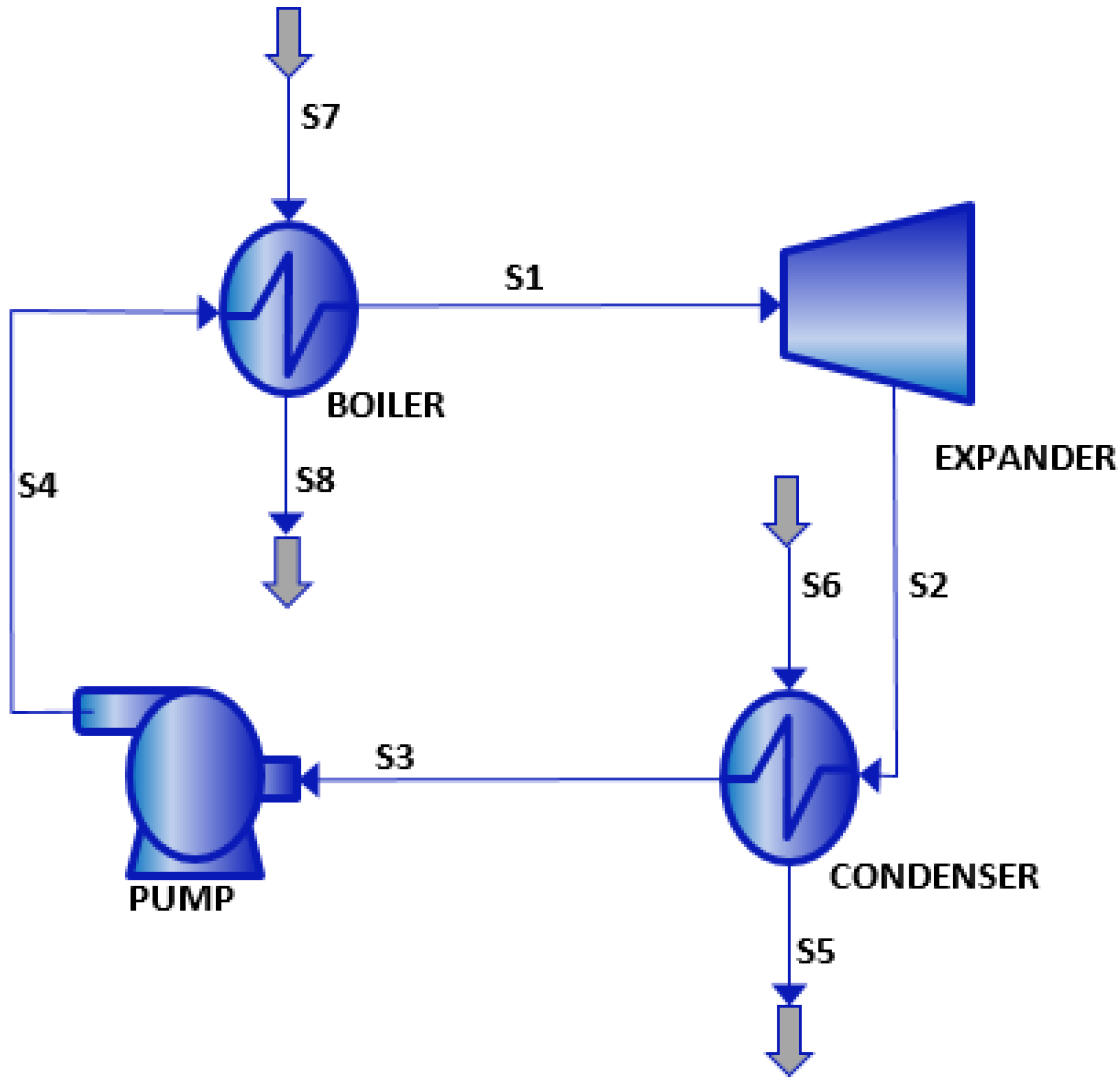
Figure 1. General system layout.

Figure 1. General system layout.

It is a closed cycle plant composed by four (4) elementary processes:

• S3–S4 Compression in a Pump: a feed pump pressurizes liquid working fluid.
• S4–S1 Vaporization in a Boiler: the liquid working fluid absorbs thermal energy and vaporizes into the vapor state. The heat exchange from the heat carrier fluid to the working fluid is completed via evaporators.
• S1–S2 Expansion in an Expander: power producing process. The heat energy of the working fluid is converted into mechanical energy by an expander; then, an alternator (not represented) converts this mechanical energy into electricity.
• S2–S3 Condensation in a Condenser: heat-rejecting process. The vapor fluid condenses into the liquid state.

3. Thermodynamic Analysis of the ORC

3.1. Simulations

This simulation objective [1] is the detailed study of the cycle sensitivity to the different process parameters variations: a sensitivity analysis provides a very useful information and suggestions, before performing an optimization procedure. We will describe the following simulations:

• Operating fluid:

  -

  Water;

  -

  R134a (organic fluid);

  -

  R245fa (organic fluid).

• Cases:

ORC plant, with at least P_net = 2 kW, thermal source: Diesel ICE, operating with the different chosen fluids.

Data and Design Constraints

As it has been repeatedly pointed out, the main objective of this paper is to study the feasibility of an ORC, operating with a IFR turbine, which recovers energy from the heat contained in the exhaust gas of a diesel engine [1,4,14], usually adopted by commercial passenger sedans (a typical 1400 cc Ford engine, Table 1), to produce electricity. The engine specifications are known and all exhaust gas data are available [1]:

• mass flow rate (kg/s);
• temperature (K);
• pressure (Pa);
• composition.

For the cooling process, water at 288 K and 200 kPa is chosen for this initial approach (the water is the most common and available fluid in almost every system). At the moment, the water side process and configuration and devices do not concern this study. As a general rule, low-pressure levels are maintained to avoid possible explosions or breaking material failures. On the other hand, this allows the use of less resistant and more economical materials in the manufacture of the system. Temperature levels are maintained below 353 K for organic fluids and 473 K for water, for the same reason previously explained. The mass flow rate of process fluid must not exceed 0.5 kg/s (design constraint); thus avoiding the use of big fluid tanks, which increases the size of the entire plant. During the design procedure, we tried to respect the rotational speed limit (30,000 rpm or about 3500 rad/s).

Table 1. Thermal source main data [1].

Parameter	Diesel engine
Mass flow rate (kg/s)	0.15
Exhausts temperature (K)	845
Pressure (Pa)	200
Average composition (per cent by volume)	CO = 0.041; CO2 = 2.74; O2 = 17.14, CxHy ≤ 0.03

Table 1. Thermal source main data [1].

Parameter	Diesel engine
Mass flow rate (kg/s)	0.15
Exhausts temperature (K)	845
Pressure (Pa)	200
Average composition (per cent by volume)	CO = 0.041; CO2 = 2.74; O2 = 17.14, CxHy ≤ 0.03

3.2. Process Simulation with PRO/II^®

To analyze the ORC plant performance a steady state simulation of the plant has been performed, with the PRO/II^® Process Simulator [15]. The software has been developed by Invensys^TM (London, UK) and runs in an interactive Windows-based GUI environment. This steady-state simulator performs rigorous mass and energy balances for a wide range of processes.

4. The Plant Layout and Simulations Results

The studied elements were the boiler, the turbine and the condenser. For the boiler, at a fixed temperature (maximum temperature) and pressure, the mass flow rate was increased until the program gives an error in the process simulation. Then, the pressure is increased maintaining the same temperature and the loop until the mass flow rate starts again. The iteration process continues until the maximum fixed pressure is reached; at this point the temperature is decreased by 10 °C and the whole process is carried out once more.

Regarding the turbine, it was studied individually. The main objective was to understand the required pressures and temperature to produce a desired rated power, varying the mass flow rate.

Finally, for the condenser a similar process has been performed. In this case, at a fixed pressure and turbine outlet temperature, the condensation temperature at the outlet (hot side) has been fixed, and the mass flow rate is increased until an error occurs in the simulation. Then, the condenser inlet temperature (hot side) has been varied and the checking of the mass flow rate starts again. Once a certain temperature was reached at the inlet, the pressure is modified and the process was repeated. The “quasi-optimal” operating conditions have been reached as a compromise between the different requirements; once all values have been set, the system has been assembled and then simulated.

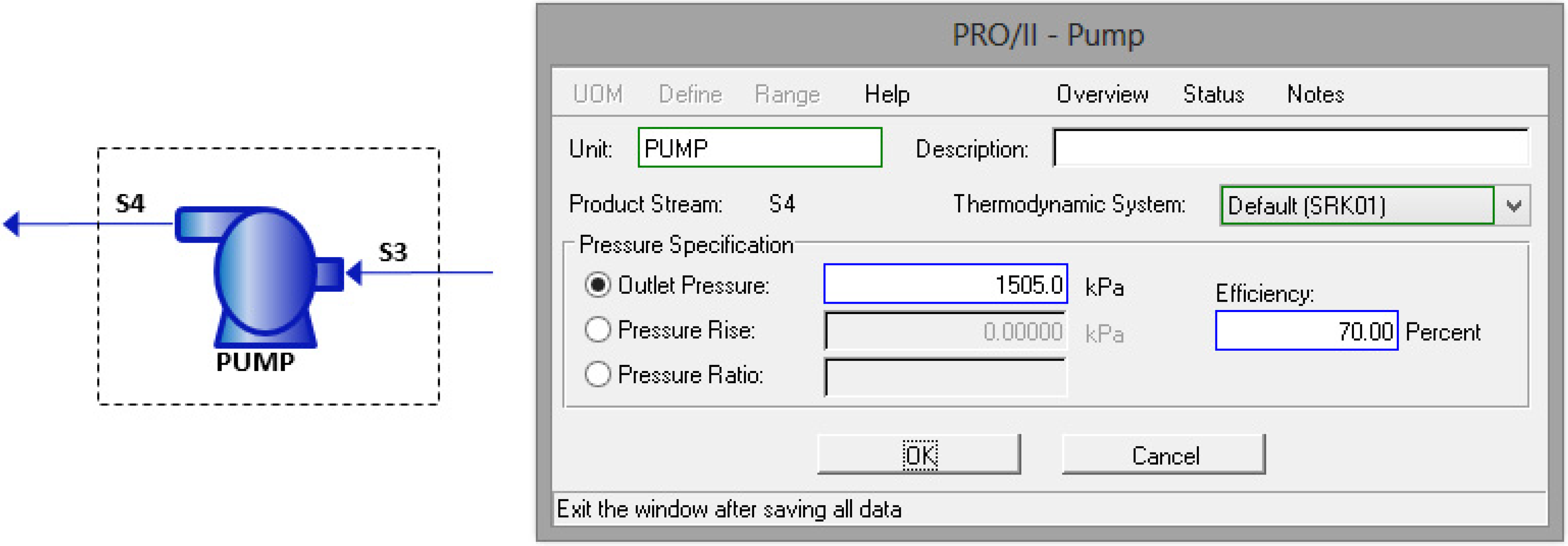
This first part was very important, because it allowed us to set and fix some operating parameters for each component, which are fundamental requirements for the subsequent sensitivity analysis. The components’ parameters set are:

Expander (Figure 2):

• Outlet pressure;
• Adiabatic efficiency;
• Estimated outlet temperature.

Condenser (Figure 3):

• Hot products temperature (outlet temperature of the working fluid).

Pump (Figure 4):

• Outlet pressure;
• Efficiency.

Boiler (Figure 5):

• Cold products temperature (outlet temperature of the working fluid).

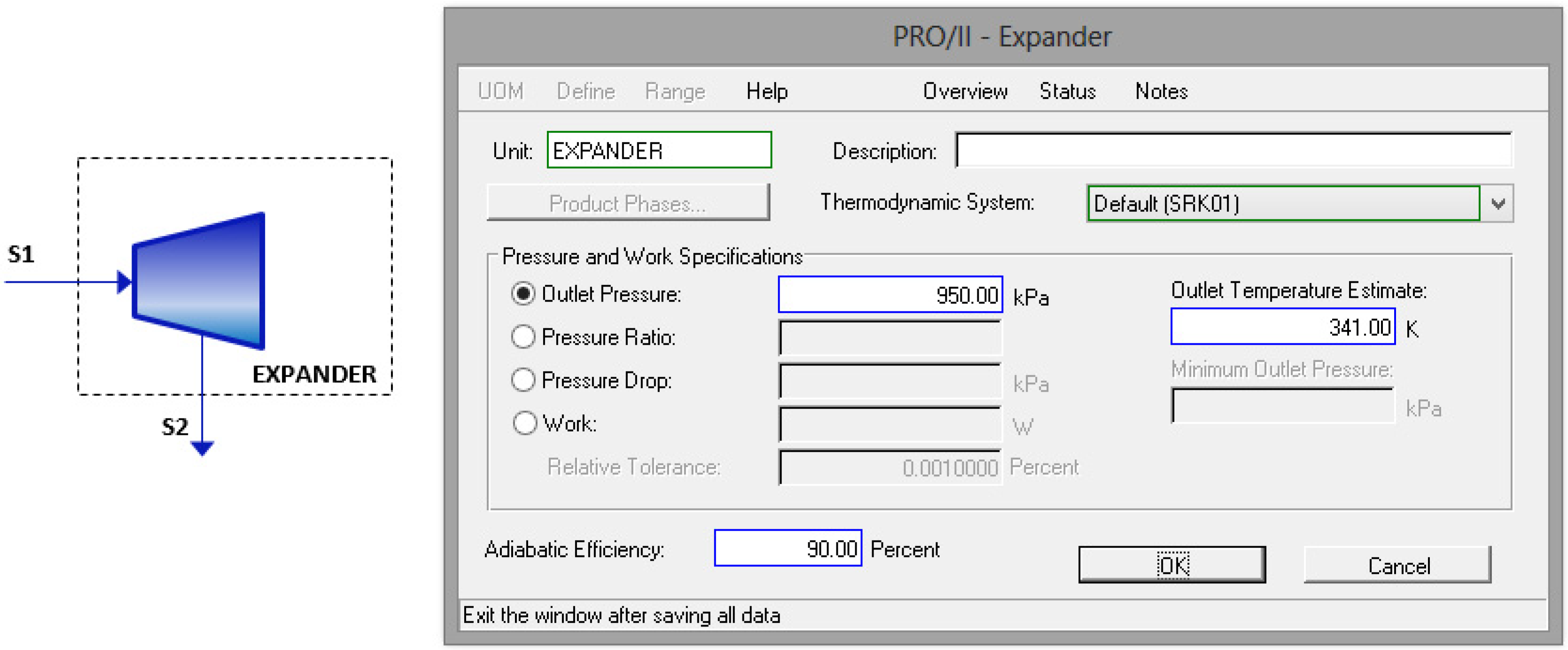
Figure 2. Expander properties selection.

Figure 2. Expander properties selection.

Figure 3. Condenser properties selection.

Figure 3. Condenser properties selection.

Figure 4. Pump properties selection.

Figure 4. Pump properties selection.

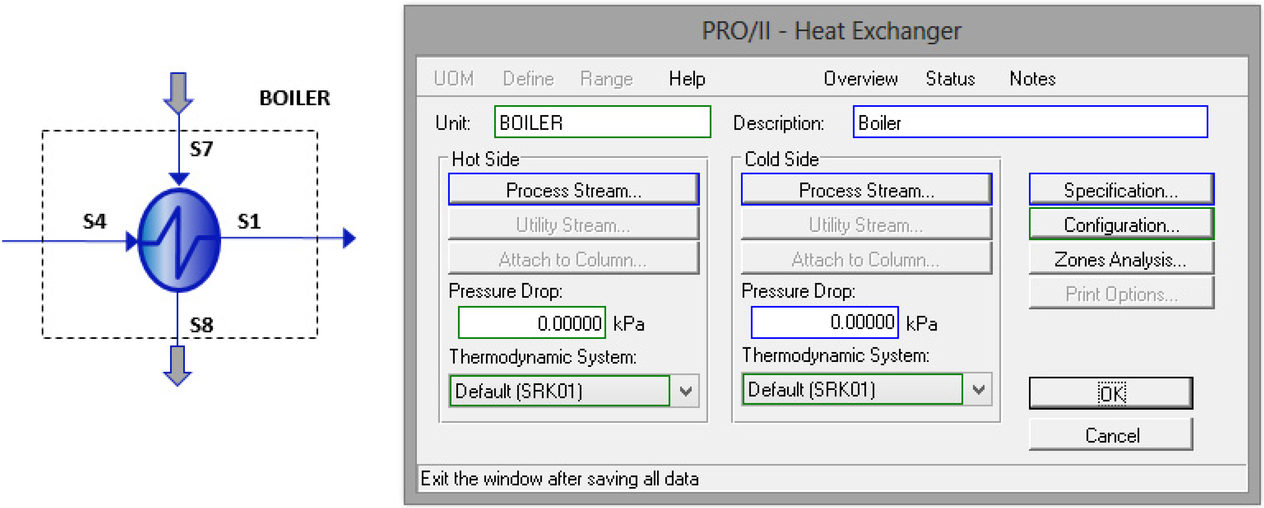
Figure 5. Boiler properties selection.

Figure 5. Boiler properties selection.

On the other hand, by analyzing the various inlet and outlet flows and the stream connections, from adopted components, the following parameters have been set:

Turbine Inlet (S1):

• temperature;
• pressure;
• mass flow rate;
• fluid composition.

Exhaust gas (S7):

• temperature;
• pressure;
• mass flow rate;
• composition.

Cooling water (S6):

• temperature;
• pressure;
• mass flow rate.

Hereafter, the results of one of the several simulations carried out for each working fluid, are reported. The ORC simulations results are presented in Table 2. The table provides all the operating parameters of the system. At the moment reviews or comparisons with experimental or actual operating data cannot be performed: in fact, at this range, there are no operating systems, but only prototypes or test benches. A sort of evaluation by simulating the same system with other codes was carried out. This comparison is not shown, because the authors believe that the attention can be shifted on the simulation and not to the project of turbo-expander.

Table 2. ORC with different working fluids.

Operating parameters	Units	R134a	R245fa	Water
ṁ gas	(kg/s)	0.15	0.15	0.15
P Inlet gas	(kPa)	200	200	200
T Inlet gas	(K)	845	845	845
P Outlet gas	(kPa)	200	200	200
ṁ	(kg/s)	0.38	0.35	0.032
Boiler inlet temperature	(K)	307	313	386
Expander inlet temperature	(K)	333	345	433
Expander outlet temperature	(K)	315	326	399
Condenser outlet temperature	(K)	307	313	386
Boiler inlet pressure	(kPa)	1500	612	310
Expander inlet pressure	(kPa)	1500	612	310
Expander outlet pressure	(kPa)	950	300	210
Condenser outlet pressure	(kPa)	950	300	210
Power output	(kW)	3.3	4.46	2.08
Power adsorbed by pump	(kW)	0.3	0.18	0.004

Table 2. ORC with different working fluids.

Operating parameters	Units	R134a	R245fa	Water
ṁ gas	(kg/s)	0.15	0.15	0.15
P Inlet gas	(kPa)	200	200	200
T Inlet gas	(K)	845	845	845
P Outlet gas	(kPa)	200	200	200
ṁ	(kg/s)	0.38	0.35	0.032
Boiler inlet temperature	(K)	307	313	386
Expander inlet temperature	(K)	333	345	433
Expander outlet temperature	(K)	315	326	399
Condenser outlet temperature	(K)	307	313	386
Boiler inlet pressure	(kPa)	1500	612	310
Expander inlet pressure	(kPa)	1500	612	310
Expander outlet pressure	(kPa)	950	300	210
Condenser outlet pressure	(kPa)	950	300	210
Power output	(kW)	3.3	4.46	2.08
Power adsorbed by pump	(kW)	0.3	0.18	0.004

5. Preliminary Design of the Expander

Once the energy recovery system thermodynamic feasibility had been checked, the next step was to start to design the expander. Radial centripetal turbines are suitable for multiple uses in the field of aeronautics, aerospace, and other areas where compact power sources are needed. This type of turbines are characterized by high efficiency, ease of production and operative reliability. In this work the general procedure to design a 90° Inward-Flow Radial (IFR) turbine is shown. The whole design is based on the Rohlik procedure for radial turbine design [16]. The reasons of this choice are the fact that the procedure defined by Rohlik is one of the most detailed and described.

By interviewing various manufacturers (GE, Siemens, Green Turbine, Infinity Turbine, etc.), we have confirmed, inasmuch as possible, the use of this procedure. In addition, we should always remember, that in this field, the screw and scroll expander have been used. Few papers describe the possible use or how to design a radial stage for a steam expander. Our target is to study the feasibility of this design procedure.

5.1. Rohlik’s Work

Adopting Rohlik’s [16] analytical studies on radial centripetal turbines performance, optimal geometry for different applications has been calculated, each one identified by characteristic parameter called “specific speed” (Ωs):

$$\text{Ωs}={\left(2\right)}^{\frac{7}{2}}\text{*}{\left(\text{π}\right)}^{\frac{1}{2}}\text{*}{\left(\frac{4\text{*}{({\text{tan α}}_1^c)}^2}{{\left(\frac{{\text{D}}_{2\text{mid}}}{{\text{D}}_1}\right)}^2}-1\right)}^{\frac{1}{4}}\text{*}{\left(\frac{{\text{b}}_2}{{\text{D}}_{2\text{mid}}}\right)}^{\frac{1}{2}}\text{*}{\left(\frac{{\text{D}}_{2\text{mid}}}{{\text{D}}_1}\right)}^{\frac{3}{2}}\text{*}{\left(\frac{{\text{U}}_1}{{\text{C}}_{\text{sp}}}\right)}^{\frac{3}{2}}$$

(1)

In this study, Rohlik considered five different types of losses:

• stator losses,
• impeller losses,
• tip clearance losses (gap between impeller and the machine stationary walls in order to avoid friction losses),
• gas leakage on seals and
• Kinetic energy losses at outlet.

Then he calculates the efficiency of a different variety of operating turbines, characterized by a “Specific Speed (Ωs)” between 0.12 and 1.34.

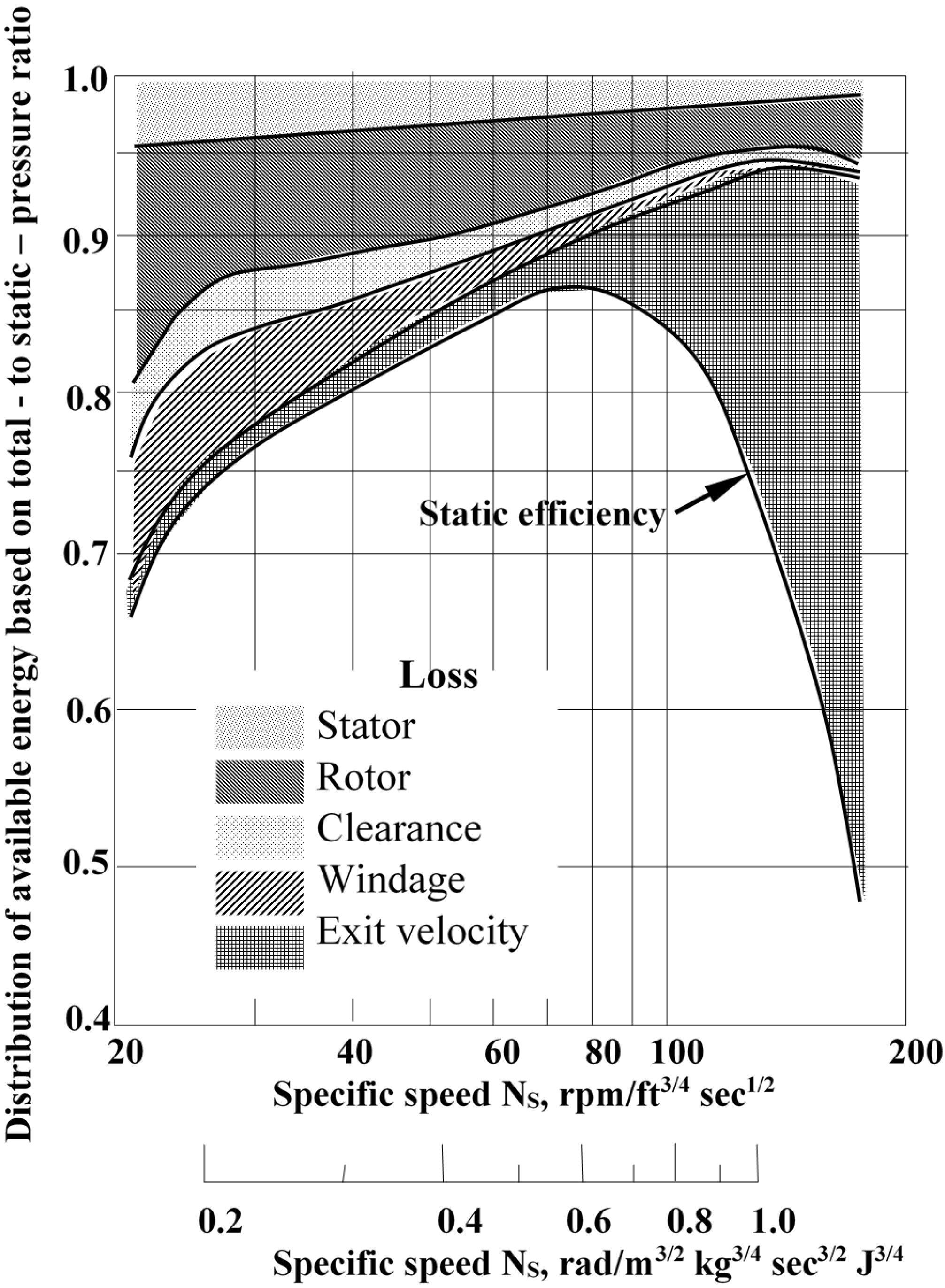
As an additional result, Rohlik developed a series of figures (Figure 6 and Figure 7) that relate this characteristic parameter (Ωs) with the different necessary geometric ratios and other parameter values to obtain the maximum turbine efficiency.

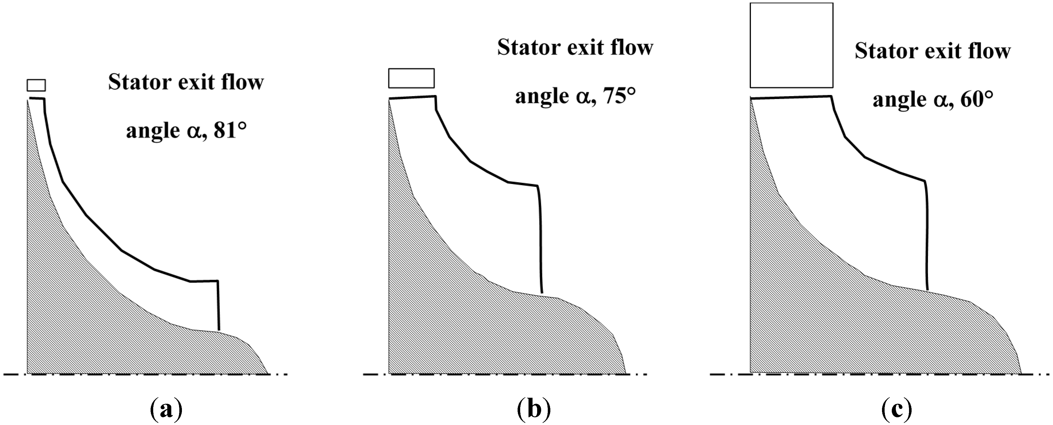
The specific speed value provides a general indication about the geometry of the turbine: low values of this parameter are associated to a relatively small areas of transition, while higher values are associated to larger areas of transition (Figure 8). In addition, this characteristic parameter can supply a first indication of the maximum efficiency that is possible to reach.

The goal of this procedure is to obtain maximum efficiency from each family of turbines analyzed and tested. Consequently the “quasi-optimal” configuration of the impeller.

Figure 6. Distribution of losses along envelope of maximum total-to-static efficiency [14,15,16].

Figure 6. Distribution of losses along envelope of maximum total-to-static efficiency [14,15,16].

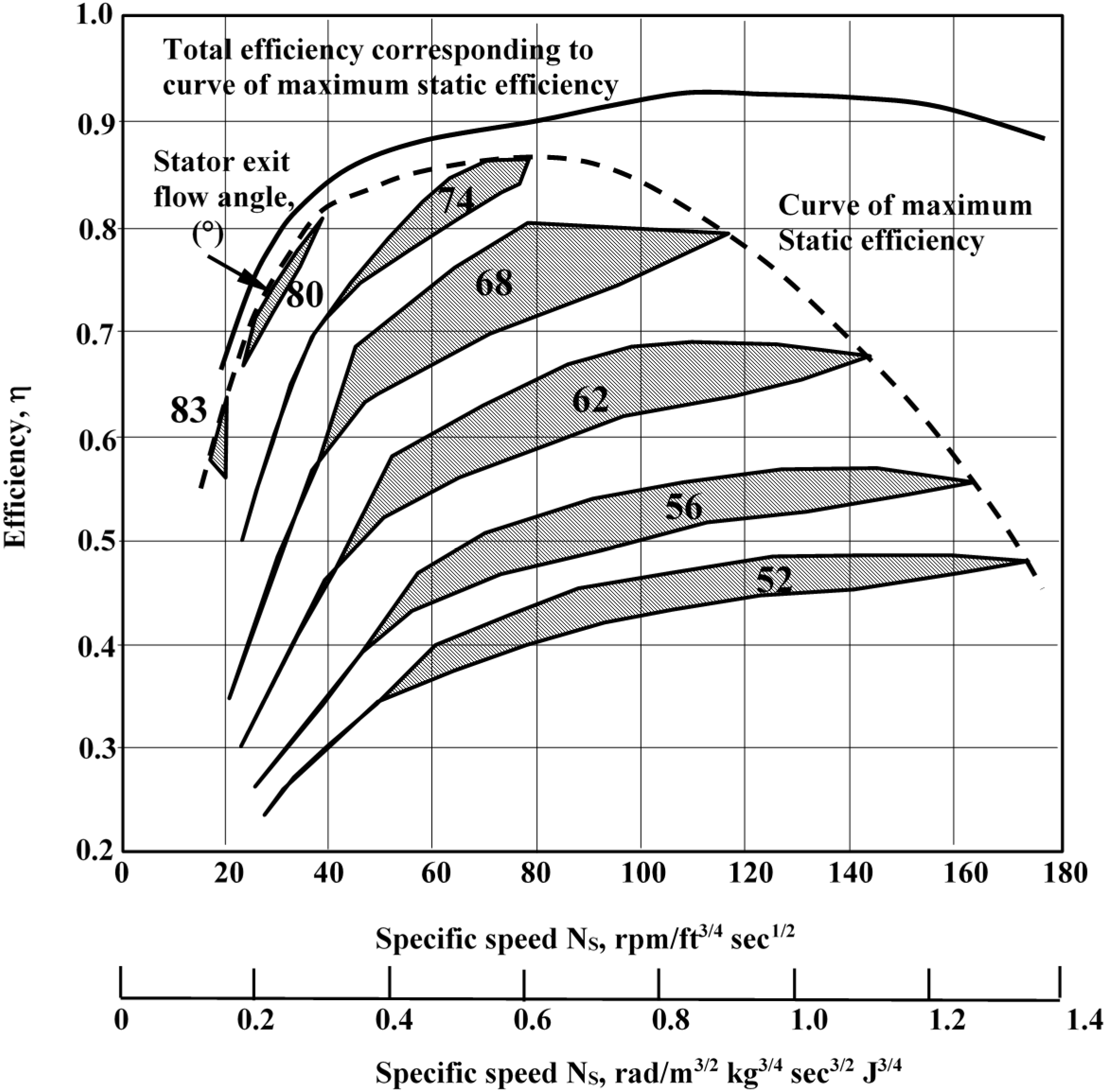
Figure 7. Efficiency vs. Absolute flow angle at rotor’s inlet, depending on Ωs [14,15,16].

Figure 7. Efficiency vs. Absolute flow angle at rotor’s inlet, depending on Ωs [14,15,16].

Figure 8. Relationship between Ωs and the general geometry of the rotor [9,16,17]. (a) Specific speed, 30 rpm per foot^3/4 per s^1/2 (0.23 rad/(m^3/2·kg^3/4·s^3/2·J^3/4)); blade-jet speed ratio, 0.68; (b) Specific speed, 70 rpm per foot^3/4 per s^1/2 (0.54 rad/(m^3/2·kg^3/4·s^3/2·J^3/4)); blade-jet speed ratio, 0.70; (c) Specific speed, 150 rpm per foot^3/4 per s^1/2 (1.16 rad/(m^3/2·kg^3/4·s^3/2·J^3/4)); blade-jet speed ratio, 0.62.

Figure 8. Relationship between Ωs and the general geometry of the rotor [9,16,17]. (a) Specific speed, 30 rpm per foot^3/4 per s^1/2 (0.23 rad/(m^3/2·kg^3/4·s^3/2·J^3/4)); blade-jet speed ratio, 0.68; (b) Specific speed, 70 rpm per foot^3/4 per s^1/2 (0.54 rad/(m^3/2·kg^3/4·s^3/2·J^3/4)); blade-jet speed ratio, 0.70; (c) Specific speed, 150 rpm per foot^3/4 per s^1/2 (1.16 rad/(m^3/2·kg^3/4·s^3/2·J^3/4)); blade-jet speed ratio, 0.62.

5.2. General Procedure

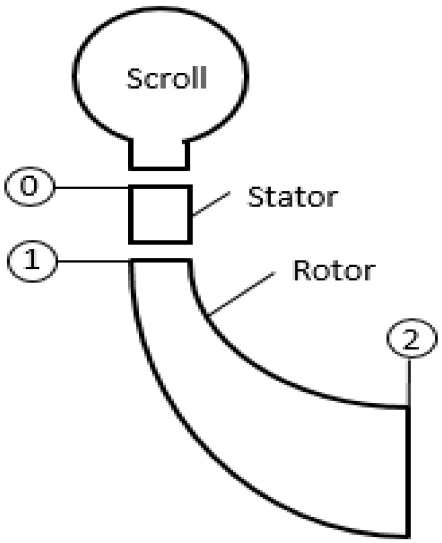
First, we have to define the fluid’s states in it pass through the turbine (Figure 9) and then, to establish the initial assumptions needed to start the design process.

Figure 9. Turbine general scheme.

Figure 9. Turbine general scheme.

• The outlet nozzle angle is taken as the optimal value determined by ROHLIK: α₁ = 16°;
• The meridian diameter of the rotor outlet section to rotor inlet diameter ratio is:

  $$\frac{{\text{D}}_{2\text{mid}}}{{\text{D}}_1}=0.49$$

  (2)
• The rotor inlet beta angle is fixed at 90°, imposed by the material characteristics and gas temperature:

  $${\text{β}}_1=90° \to {\text{ψ}}_1=1;$$
• Rotor outlet α₂ is assumed zero (axial flow at outlet):

  $${\text{α}}_2=90° \to {\text{ψ}}_2=0$$
• Rotor outlet relative velocity at midspan (W_2mid) is two times the rotor inlet relative velocity (W₁):

  $${\text{W}}_{2\text{mid}}=2 {\text{W}}_1$$

  (3)

With these initial inputs, the “Spouting Velocity (C_SP)” was calculated. Assuming an initial R_ρ equal to 0.5, is possible to calculate T₁ and P₁ that represent the inlet fluid conditions. Now, it is possible to find fluid density on state “1” (ρ₁) and then Q₁. Remembering the Euler work equation and neglecting the dynamic enthalpy (as an initial approach), the value of peripheral velocity U₁ can be obtained:

$${\text{h}}_0-{\text{h}}_2={\text{U}}_1^2·{\text{ψ}}_1\to {\text{ U}}_1=\sqrt{\frac{{\text{h}}_0-{\text{h}}_2}{{\text{ψ}}_1}}$$

(4)

With U₁, the rotor inlet diameter has so calculated:

$${\text{U}}_1=\frac{{\text{D}}_1}{2}·\text{ ω }\to {\text{ D}}_1=\frac{2·{\text{U}}_1}{\text{ω}}$$

(5)

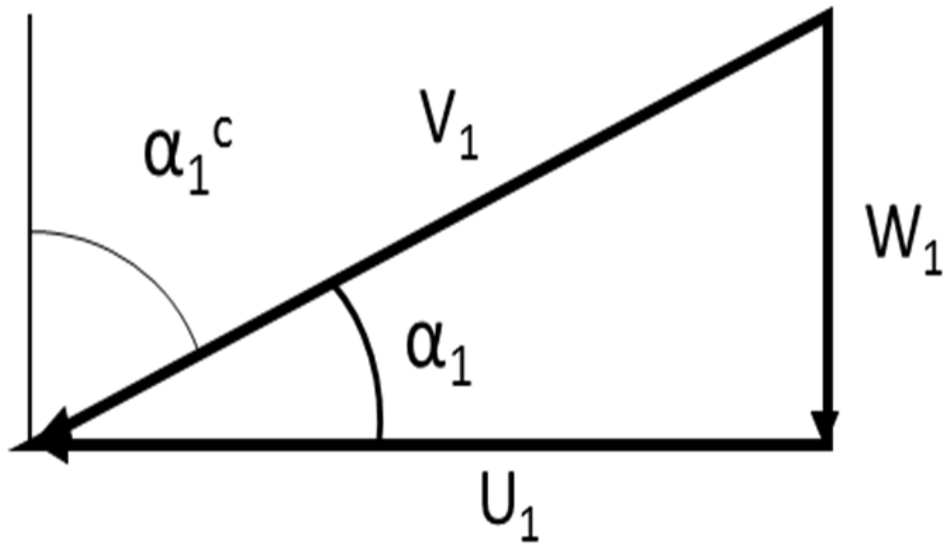
With α₁ and from geometry of the velocity triangle (Figure 10) we obtain the rest of the kinematic parameters.

Then the blade height, at inlet, is computed as:

$${\text{b}}_1=\frac{{\text{Q}}_1}{\text{π}·{\text{V}}_{\text{m}1}·{\text{D}}_1·{\text{δ}}_{1-2}}$$

(6)

where ${\delta }_{1-2}$ is a blockage coefficient that considers the part of the area occupied by the blade.

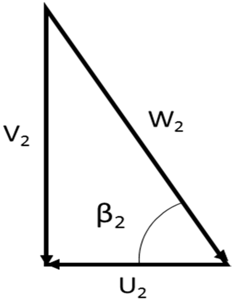
Once D₁ is known, we compute D_2mid from initial assumption, and then with ω and D_2mid, U_2mid. From geometry is possible to determine the rest of the kinematic parameters at mid-span (Figure 11) section.

Figure 10. General inlet velocity triangle.

Figure 10. General inlet velocity triangle.

Figure 11. General outlet velocity triangle.

Figure 11. General outlet velocity triangle.

The blade height, at outlet, is computed as:

$${\text{b}}_2=\frac{{\text{Q}}_2}{\text{π}·{\text{V}}_{\text{m}2\text{mid}}·{\text{D}}_{2\text{mid}}·{\text{δ}}_{1-2}}$$

(7)

The outlet hub and shroud diameter:

D_2shroud = D_2mid + b₂; D_2hub = D_2mid – b₂

(8)

Then U_2hub and U_2shroud:

$${\text{U}}_{2\text{shroud}}=\frac{{\text{D}}_{2\text{shroud}}}{2}\text{ω};{\text{U}}_{2\text{hub}}=\frac{{\text{D}}_{2\text{hub}}}{2}\text{ω}$$

(9)

Flow coefficients (φ) at outlet section can be computed. From geometrical considerations, it is possible to obtain the rest of the operative data for hub and shroud. After that, it is necessary to verify the principal limits that Rohlik indicates on his work, that are:

$$\frac{{\text{D}}_{2\text{hub}}}{{\text{D}}_{2\text{shroud}}}\ge 0,4;\frac{{\text{D}}_{2\text{shroud}}}{{\text{D}}_1}\le 0,7$$

The Rohlik specific velocity (an equation proposed on Dixon’s book [18]) is:

$${\text{Ω}}_{\text{s}}=2.11·{\left(\frac{{\text{c}}_2}{{\text{c}}_0}\right)}^{1/2}·{\left(\frac{{\text{A}}_2}{{\text{A}}_{\text{d}}}\right)}^{1/2}$$

(10)

where c₀ is the spouting velocity and:

$${\text{A}}_2=\frac{{\text{Q}}_2}{{\text{c}}_2};{\text{ A}}_{\text{d}}=\frac{\text{π}·{\text{D}}_1^2}{4}$$

(11)

This specific velocity is considered only as a “reference value”, to determine how effective our procedure is; in any case, it is a key parameter on this study. The new reaction degree at mid-span is calculated and a second iteration have been made, to adjust the parameter values. The number of blades for the rotor and stator can be computed as follows:

$${\text{Z}}_{\text{rot}}\ge \frac{\text{π}}{30}·\left({\text{α}}_1^{°}+20\right)·\cot {\text{α}}_1$$

(12)

$${\text{Z}}_{\text{sta}}\approx {\text{ Z}}_{\text{rot}}-2$$

(13)

For nozzle calculation, we have assumed:

$$(\text{a}){\text{ b}}_0={\text{b}}_1;(\text{b}){\text{ α}}_{1\text{sta}}={\text{α}}_1$$

(14)

$$(\text{c})\frac{{\text{D}}_0}{{\text{D}}_{1\text{sta}}}=1.3;(\text{d}){\text{ δ}}_{0-1}=0.85$$

(15)

where:

$${\text{D}}_{1\text{sta}}={\text{D}}_1+0.004(\text{m})$$

(16)

Finally, the value of α₀ and velocity components of the fluid at nozzle inlet have been computed:

$${\text{V}}_{0\text{m}}=\frac{{\text{ρ}}_1·{\text{ V}}_{1\text{m}}·{\text{r}}_{1\text{sta}}·{\text{b}}_{1\text{sta}}·{\text{δ}}_{0-1}}{{\text{ρ}}_0·{\text{r}}_0·{\text{b}}_0·{\text{δ}}_{0-1}}$$

(17)

$${\text{V}}_{0\text{t}}=\frac{{\text{V}}_{0\text{m}}}{\tan {\text{α}}_0}$$

(18)

6. Expander Design Results

Using the procedure, briefly described, the main geometric parameters for the design of the expander impeller have been derived. The following results (Table 3), are obtained after an accurate “optimization” (maybe it would be better to define it as iterative optimization process) of the results, by varying the initial parameters.

Table 3. Number of triangular elements for FEM studies.

Fluid	Water	R134a	R245fa
N° elements	647070	663509	591739

Table 3. Number of triangular elements for FEM studies.

Fluid	Water	R134a	R245fa
N° elements	647070	663509	591739

7. Termo-Structural (FEM) Analysis

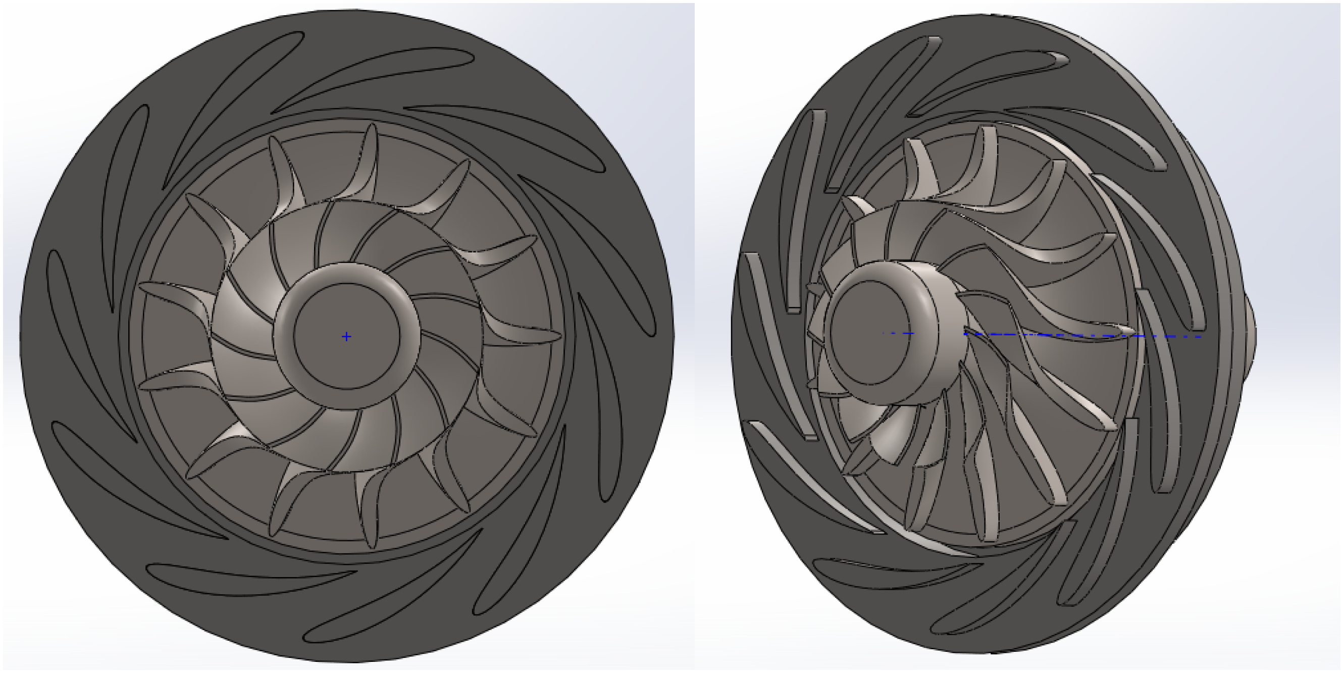
Once the impeller design procedure has been completed, a drawing, both in 2D and 3D, was made. The 3-D geometry of the turbine (Figure 12 and Figure 13) was created using a dedicated commercial software (ANSYS Blademodeler^®, ANSYS, Inc., Cecil Township, PA, USA) in which all the geometrical data is inserted [19]. The variation of the beta angle (β) along the rotor was establish by a spline curve for every layer (mid, hub and shroud) that can be configured and modified in the program. The blade profile chosen for both, the rotor and stator, was a general NACA (National Advisory Committee for Aeronautics) profile. Once the drawing has been completed, the mesh has been created. The mesh is composed by triangular elements; the number of elements is shown in Table 4.

Table 4. Expander design results.

Basic Thermodynamic Data
Fluid	R134a	R245fa	Water
T0 (K)	333	345	433
P0 (kPa)	1,500	612	310
T1 (K)	327	338	421
P1 (kPa)	1,363	501.7	272.7
T2 (K)	315	326	399
P2 (kPa)	950	300	210
Rotor Geometry
D1 (m)	0.041	0.073	0.058
b1 (m)	0.002	0.002	0.002
D2mid (m)	0.020	0.036	0.028
b2 (m)	0.006	0.007	0.005
D2hub (m)	0.014	0.029	0.023
D2shroud (m)	0.026	0.042	0.033
Zrotor	13	13	13
Velocity Triangles
ω (rpm)	42,500	30,000	84,000
V1 (m/s)	94.5	118.7	262.9
W1 (m/s)	26.0	32.7	72.5
U1 (m/s)	90.8	114.1	252.7
β1 (°)	90	90	90
φ1	0.286	0.29	0.29
V2mid (m/s)	27.0	34	75.3
W2mid(m/s)	52.0	65.4	144.9
U2mid (m/s)	44.5	55.9	123.8
α2mid (°)	90	90	90
β2mid (°)	31	31	31
φ2mid	0.61	0.61	0.61
V2shroud (ms)	27.0	34	75.3
W2shroud (m/s)	63.6	74.7	163.6
U2shroud (m/s)	57.6	66.5	145.3
α2shroud (°)	90	90	90
β2shroud (°)	25	27	27
ψ2shroud	0	0	0
φ2shroud	0.47	0.51	0.52
V2hub (m/s)	27	34	75.3
W2hub (m/s)	41.5	56.7	127.1
U2hub (m/s)	31.4	45.3	102.4
α2hub (°)	90	90	90
β2hub (°)	41	37	36
ψ2hub	0	0	0
φ2hub	0.86	0.75	0.74
Nozzle Geometry
D1sta (m)	0.045	0.077	0.061
D0 (m)	0.058	0.1	0.08
b0 (m)	0.002	0.002	0.002
α0 (°)	21	19	28
V0 (m/s)	45.9	60.1	100.5
Zstator	11	11	11

Table 4. Expander design results.

Basic Thermodynamic Data
Fluid	R134a	R245fa	Water
T0 (K)	333	345	433
P0 (kPa)	1,500	612	310
T1 (K)	327	338	421
P1 (kPa)	1,363	501.7	272.7
T2 (K)	315	326	399
P2 (kPa)	950	300	210
Rotor Geometry
D1 (m)	0.041	0.073	0.058
b1 (m)	0.002	0.002	0.002
D2mid (m)	0.020	0.036	0.028
b2 (m)	0.006	0.007	0.005
D2hub (m)	0.014	0.029	0.023
D2shroud (m)	0.026	0.042	0.033
Zrotor	13	13	13
Velocity Triangles
ω (rpm)	42,500	30,000	84,000
V1 (m/s)	94.5	118.7	262.9
W1 (m/s)	26.0	32.7	72.5
U1 (m/s)	90.8	114.1	252.7
β1 (°)	90	90	90
φ1	0.286	0.29	0.29
V2mid (m/s)	27.0	34	75.3
W2mid(m/s)	52.0	65.4	144.9
U2mid (m/s)	44.5	55.9	123.8
α2mid (°)	90	90	90
β2mid (°)	31	31	31
φ2mid	0.61	0.61	0.61
V2shroud (ms)	27.0	34	75.3
W2shroud (m/s)	63.6	74.7	163.6
U2shroud (m/s)	57.6	66.5	145.3
α2shroud (°)	90	90	90
β2shroud (°)	25	27	27
ψ2shroud	0	0	0
φ2shroud	0.47	0.51	0.52
V2hub (m/s)	27	34	75.3
W2hub (m/s)	41.5	56.7	127.1
U2hub (m/s)	31.4	45.3	102.4
α2hub (°)	90	90	90
β2hub (°)	41	37	36
ψ2hub	0	0	0
φ2hub	0.86	0.75	0.74
Nozzle Geometry
D1sta (m)	0.045	0.077	0.061
D0 (m)	0.058	0.1	0.08
b0 (m)	0.002	0.002	0.002
α0 (°)	21	19	28
V0 (m/s)	45.9	60.1	100.5
Zstator	11	11	11

Figure 12. 3D sketch for the expander stator and impeller.

Figure 12. 3D sketch for the expander stator and impeller.

Figure 13. Example of impeller mesh.

Figure 13. Example of impeller mesh.

Then, a first and preliminary thermo-structural simulation has been performed. In our case, it was divided into three successive steps: simple structural stress, thermal stress and, finally, a global stress, sum of the previous ones.

In details, the centrifugal stress has been obtained applying the respective rotational speed, with the rotational axis coinciding with the cylindrical surface that represents the axis. The constraint applied is a cylindrical support that allows movement only in the radial direction (the direction of the rotation movement of the turbine).

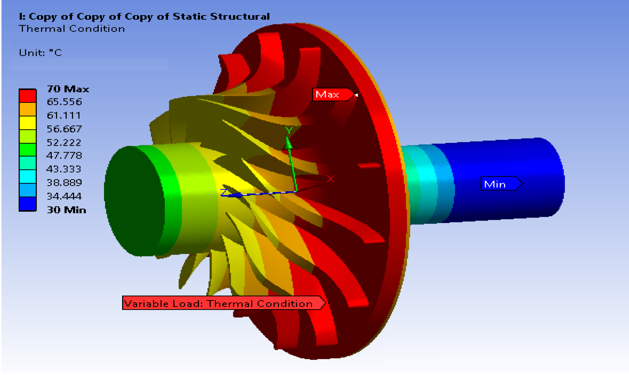
A thermal stress that varies depending Z coordinates (axial direction) has been applied. For the temperature trend, a value table, to achieve the maximum temperature at the inlet fluid section, and the minimum one at the outlet, has been used. As an example the data used for the R134a case is shown in Table 5.

Table 5. Temperature distribution table.

Z (mm)	Temperature (°C)
−15	30
0	70
20	45

Table 5. Temperature distribution table.

Z (mm)	Temperature (°C)
−15	30
0	70
20	45

An example of the distribution of the thermal load is reported in Figure 14. The last consideration is the material used. In this case, a structural steel has been used. This material is directly available in the software library and has a tensile yield strength of about 200 MPa. We know this material may not be fully compatible with the application (because it is not even stainless) but, the main objective of this preliminary study is to verify if problems with the resistance of the turbine occur, produced by the different loads. The confirmed absence of problems indicates that almost any material can be used to build the rotor.

Figure 14. Thermal load distribution on the impeller.

Figure 14. Thermal load distribution on the impeller.

8. Fluid Dynamic (CFD) Analysis

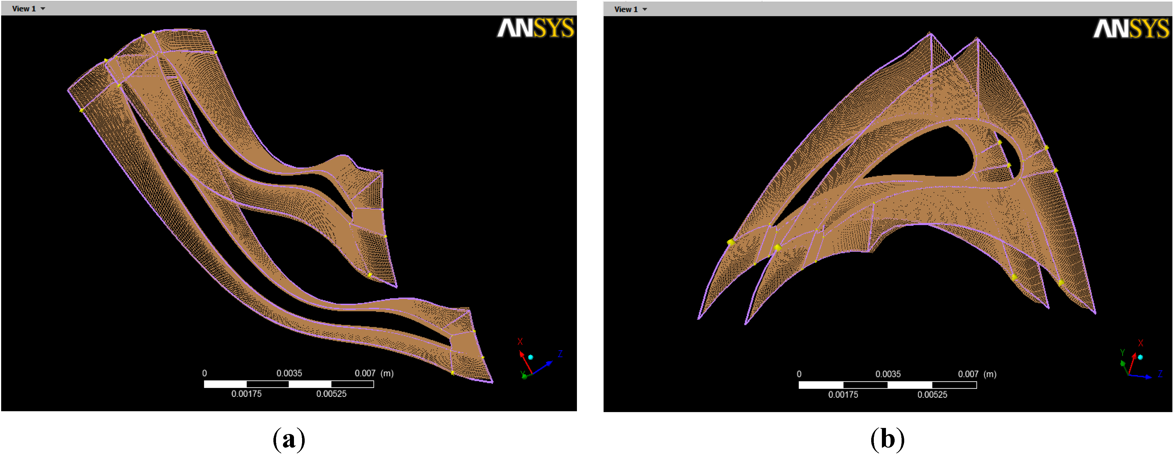
The configuration for an initial CFD analysis of the turbine has been determined. By setting the most important parameters and assigning the required boundary conditions, the mesh and the physic model were fully created. From the same 3D geometry, the first step was to create the mesh, in this case non-attached to the solid but in the region of the geometry in which the fluid will flow (considering the boundary layers in the near wall zones of the geometry like blades, shroud and hub).

Using a dedicated software (ANSYS TurboGrid) the type, amount of layers and elements our mesh will contain have to be fixed [20]. This data is shown in Table 6. The mesh is composed by quadrilateral elements and following the recommendation of the program, for the stator’s blades a J-Grid has been chosen and for the rotor’s blades an H-Grid. Once the mesh quality was verified, the resultant geometry (Figure 15) is ready for the next step, which is the configuration of the model.

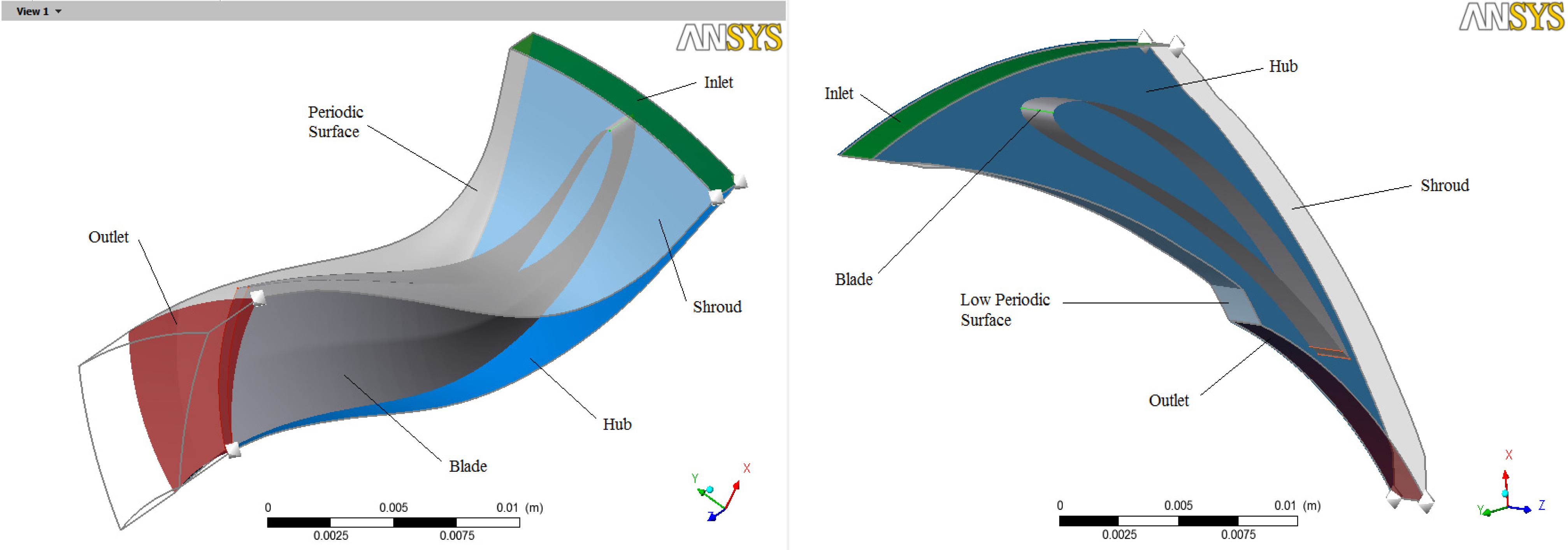
To configure the model means to set the respective boundary conditions (Table 7) for the different surfaces involved (Figure 16) and to fix some other parameters that will allow us to perform an accurate representation of the situation [21,22].

Remembering the preliminary aspect of this project the CFD study was performed as a static simulation in which the k-epsilon (k-ε) turbulent model have been selected and all the basic transport equation have been solved (momentum, continuity, total energy, etc.) for a single blade vane, to save some computational time in the simulation.

Table 6. CFD mesh data.

Water
	# of Layers	# of Nodes	# of Elements
Stator	2	381,030	345,048
Rotor	3	542,351	500,368
Total	-	923,381	845,416
R134a
	# of Layers	# of Nodes	# of Elements
Stator	2	512,730	470,008
Rotor	5	669,303	627,484
Total	-	1,181,433	1,097,492
R245fa
	# of Layers	# of Nodes	# of Elements
Stator	2	429,011	383,280
Rotor	5	538,377	498,720
Total	-	967,388	882,000

Table 6. CFD mesh data.

Water
	# of Layers	# of Nodes	# of Elements
Stator	2	381,030	345,048
Rotor	3	542,351	500,368
Total	-	923,381	845,416
R134a
	# of Layers	# of Nodes	# of Elements
Stator	2	512,730	470,008
Rotor	5	669,303	627,484
Total	-	1,181,433	1,097,492
R245fa
	# of Layers	# of Nodes	# of Elements
Stator	2	429,011	383,280
Rotor	5	538,377	498,720
Total	-	967,388	882,000

Figure 15. Example of the resultant mesh of the rotor (a) and stator (b) passage.

Figure 15. Example of the resultant mesh of the rotor (a) and stator (b) passage.

Figure 16. Rotor’s and stator’s vane surfaces.

Figure 16. Rotor’s and stator’s vane surfaces.

Table 7. Assigned boundary conditions.

Boundary Condition	Surface	Specified data
Inlet	Stator’s Inlet	ṁ, T and flow direction
Opening	Rotor’s Outlet	P and T
Wall	Hub, Shroud Blade	Static or rotating
Periodic	Limits of the blade vane	Rotational periodicity
General Connection	Stator’s Outlet-Rotor’s Inlet	-

Table 7. Assigned boundary conditions.

Boundary Condition	Surface	Specified data
Inlet	Stator’s Inlet	ṁ, T and flow direction
Opening	Rotor’s Outlet	P and T
Wall	Hub, Shroud Blade	Static or rotating
Periodic	Limits of the blade vane	Rotational periodicity
General Connection	Stator’s Outlet-Rotor’s Inlet	-

9. Results and Discussion

9.1. FEM Simulation

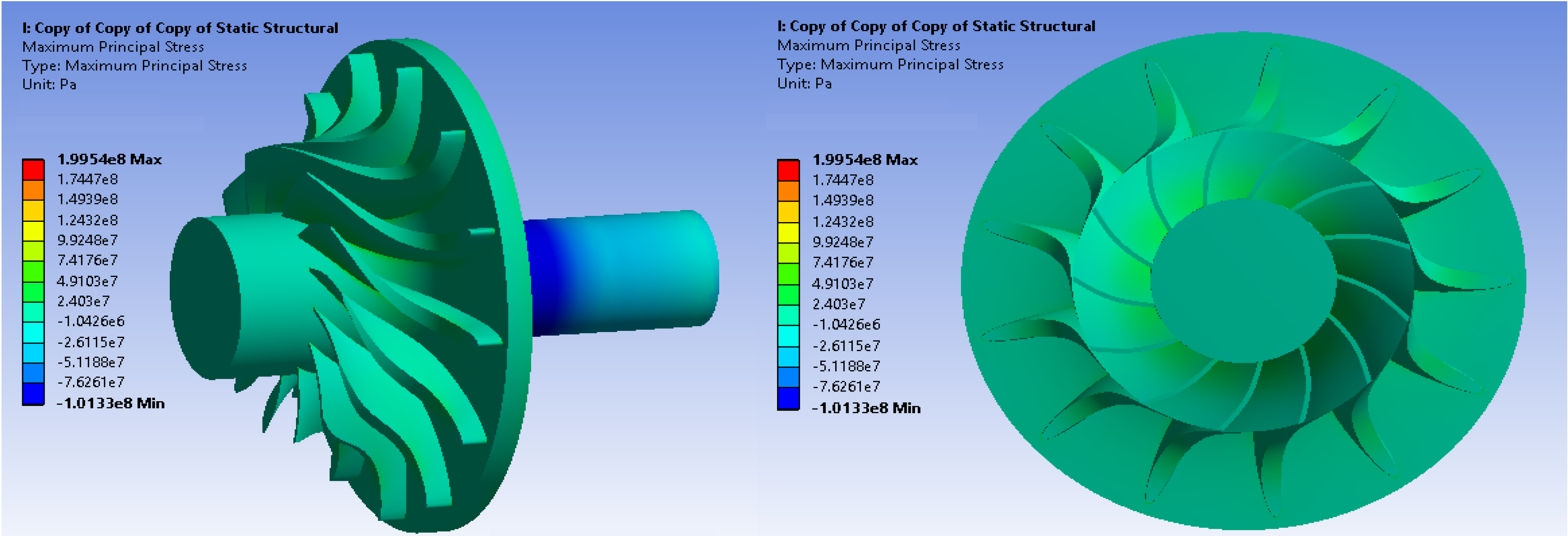
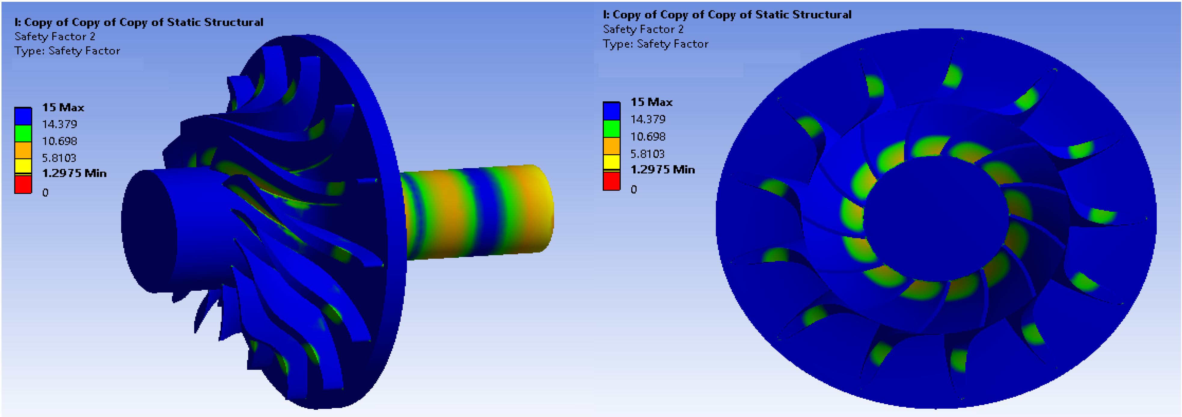
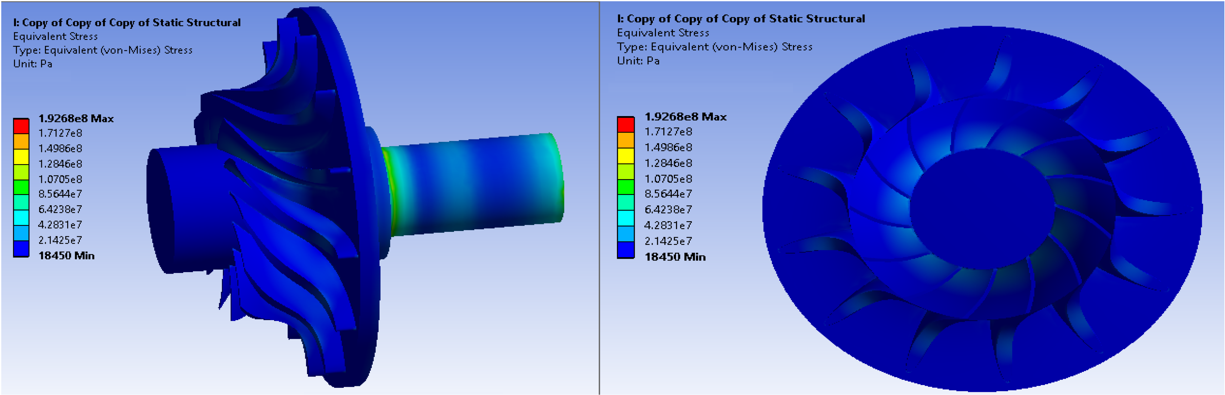
As expected, the central part of the rotor is the most stressed part, due to the centrifugal forces combined with the thermal load. Finally, to determine safely conditions, the safety factor (as the yield stress of the material divided by maximum equivalent stress) has been computed. Operating in this way, satisfactory results were achieved. The value so obtained is close to the limit conditions, but still under the limit imposed by the material strength. Figure 17, Figure 18 and Figure 19 illustrate the global stress and the displacement of the rotor.

Figure 17. Maximum global stress (R134a).

Figure 17. Maximum global stress (R134a).

Figure 18. Equivalent Von Misses stress (R134a).

Figure 18. Equivalent Von Misses stress (R134a).

Figure 19. Safety factor for final global stress (R-134a).

Figure 19. Safety factor for final global stress (R-134a).

9.2. CFD Simulation

The most important parameter in a CFD simulation is probably the mass imbalance: the smaller it is the more accurate the simulation (Table 8).

Table 8. Mass imbalance.

Fluid Case	Part	ṁ inlet (kg/s)	ṁ outlet (kg/s)	Mass imbalance (%)
Water	Stator	0.002909	−0.002908	0.034
	Rotor	0.002461	−0.0024607	0.012
R-134a	Stator	0.0345454	−0.0345426	0.008
	Rotor	0.0292283	−0.0292275	0.0027
R-245fa	Stator	0.031818	−0.031802	0.05
	Rotor	0.026909	−0.026901	0.029

Table 8. Mass imbalance.

Fluid Case	Part	ṁ inlet (kg/s)	ṁ outlet (kg/s)	Mass imbalance (%)
Water	Stator	0.002909	−0.002908	0.034
	Rotor	0.002461	−0.0024607	0.012
R-134a	Stator	0.0345454	−0.0345426	0.008
	Rotor	0.0292283	−0.0292275	0.0027
R-245fa	Stator	0.031818	−0.031802	0.05
	Rotor	0.026909	−0.026901	0.029

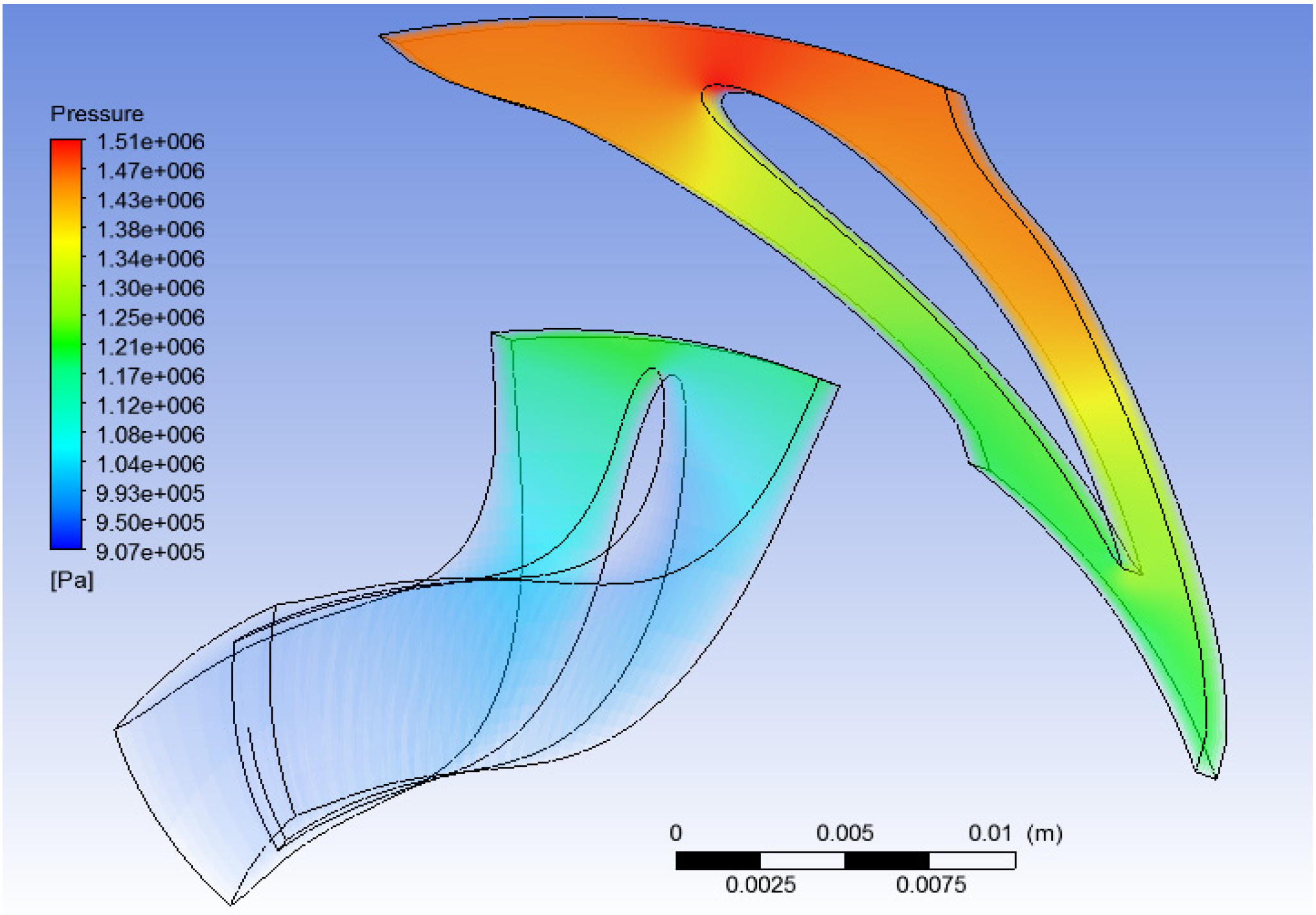
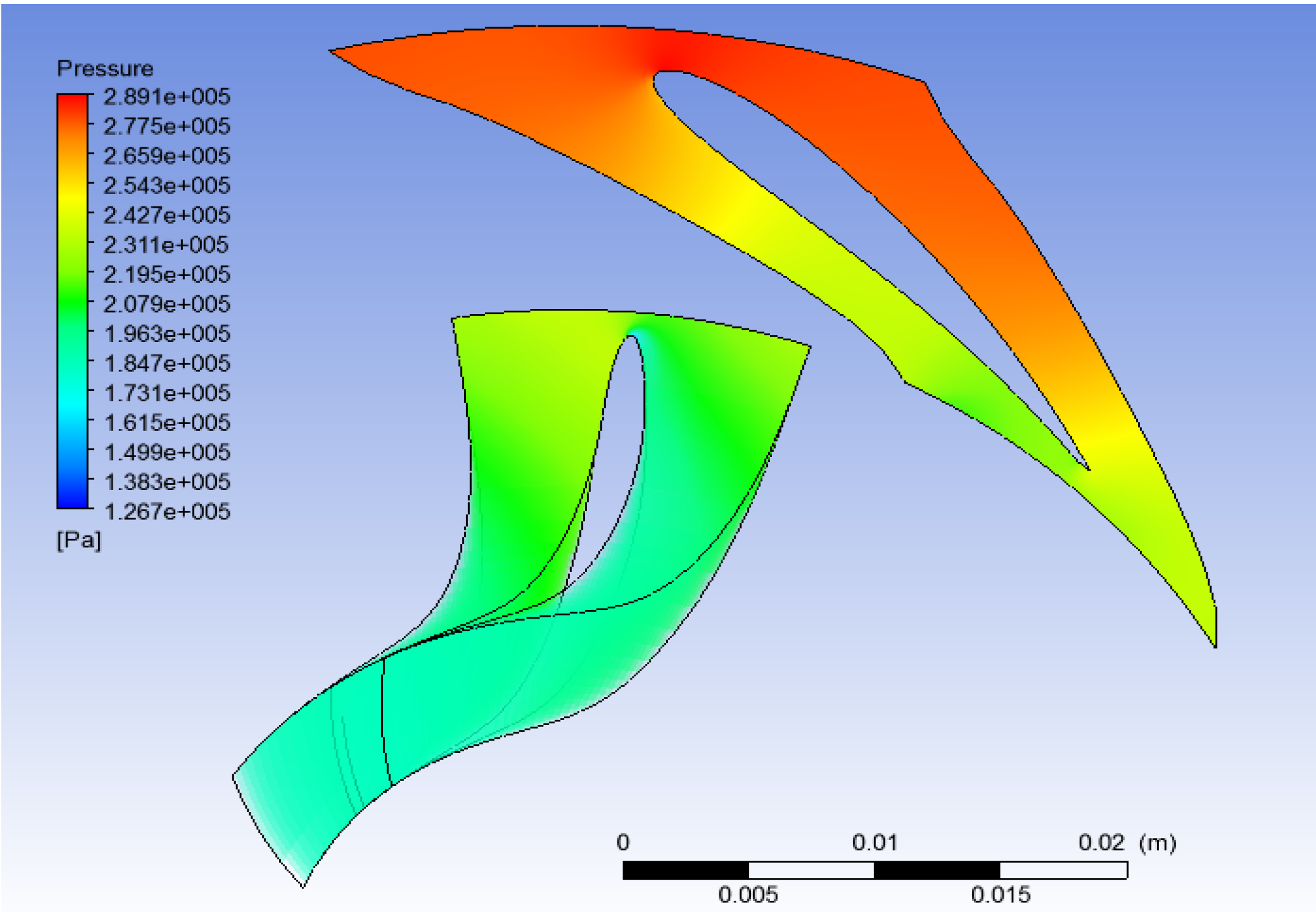
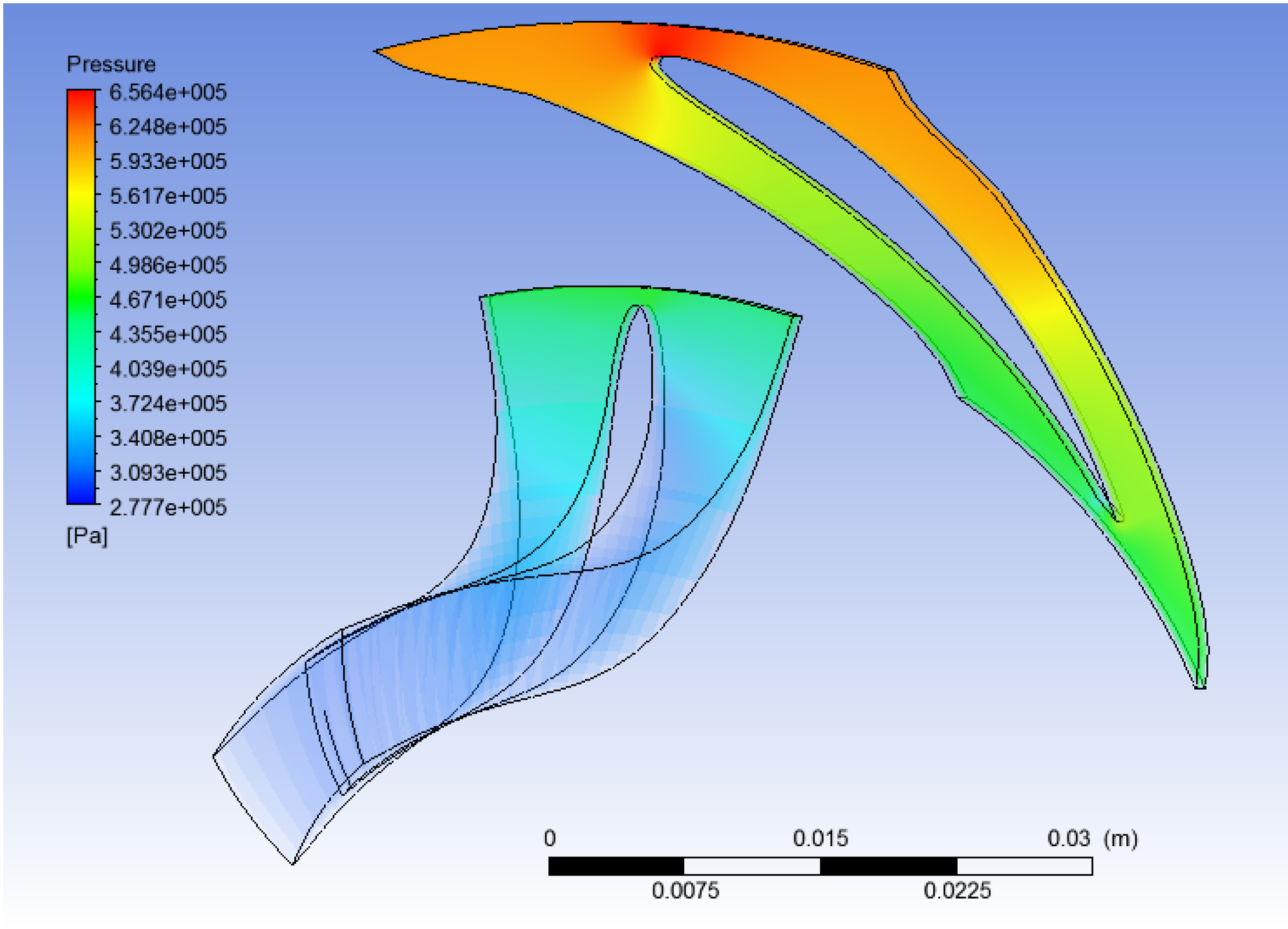
The above value of the mass imbalance indicates the numerical results are sufficiently accurate; the suggested limit in the CFX manual is (≤0.1%). The values for the pressure in each case are very similar to those assumed and calculated in the theoretical and thermodynamic part of this work—in general pressure levels are lower but with acceptable variation (Figure 20, Figure 21 and Figure 22).

Figure 20. CFD study results: Pressure (water).

Figure 20. CFD study results: Pressure (water).

Figure 21. CFD study results: Pressure (R134a).

Figure 21. CFD study results: Pressure (R134a).

Figure 22. CFD study results: Pressure (R245fa).

Figure 22. CFD study results: Pressure (R245fa).

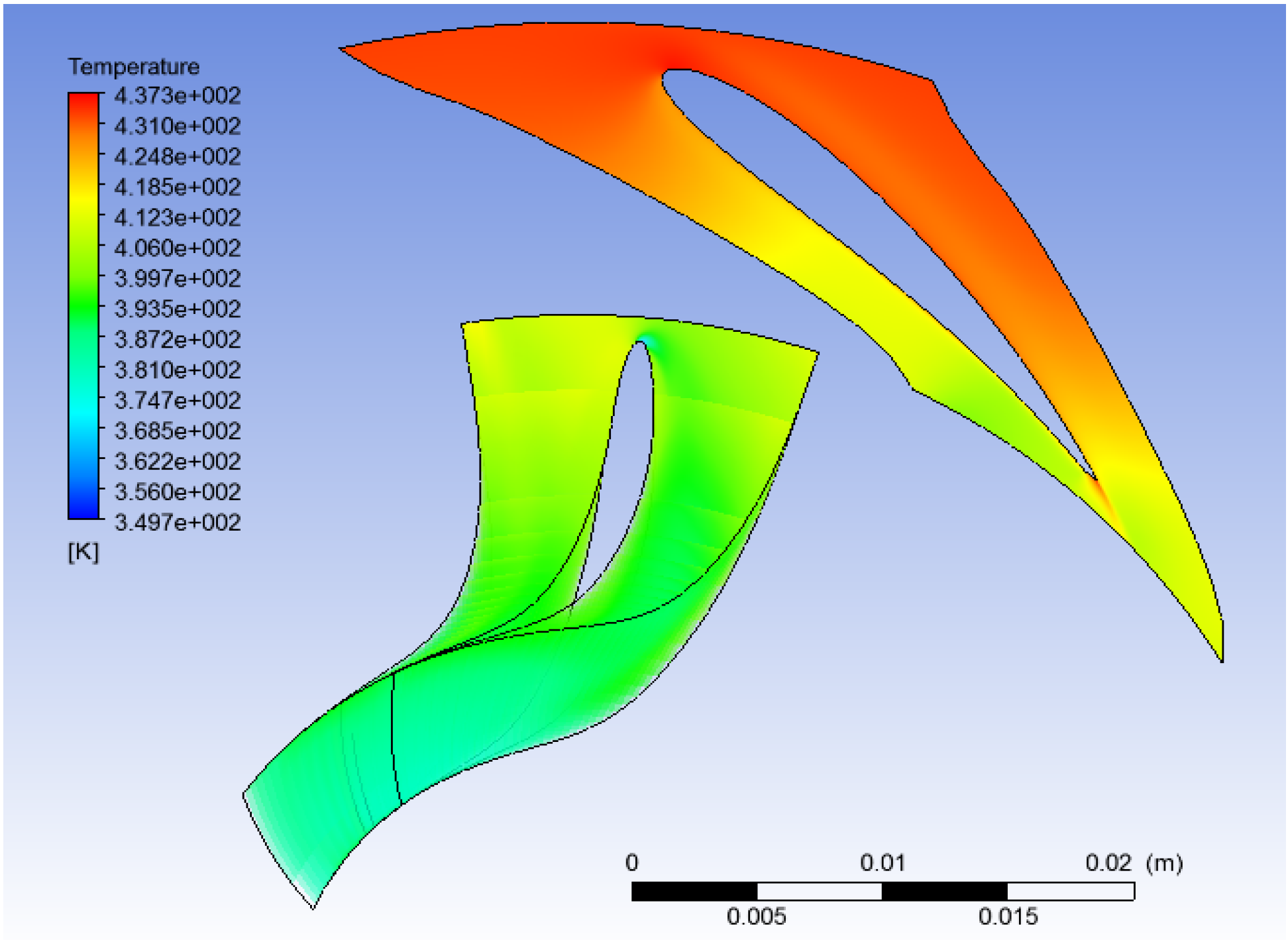
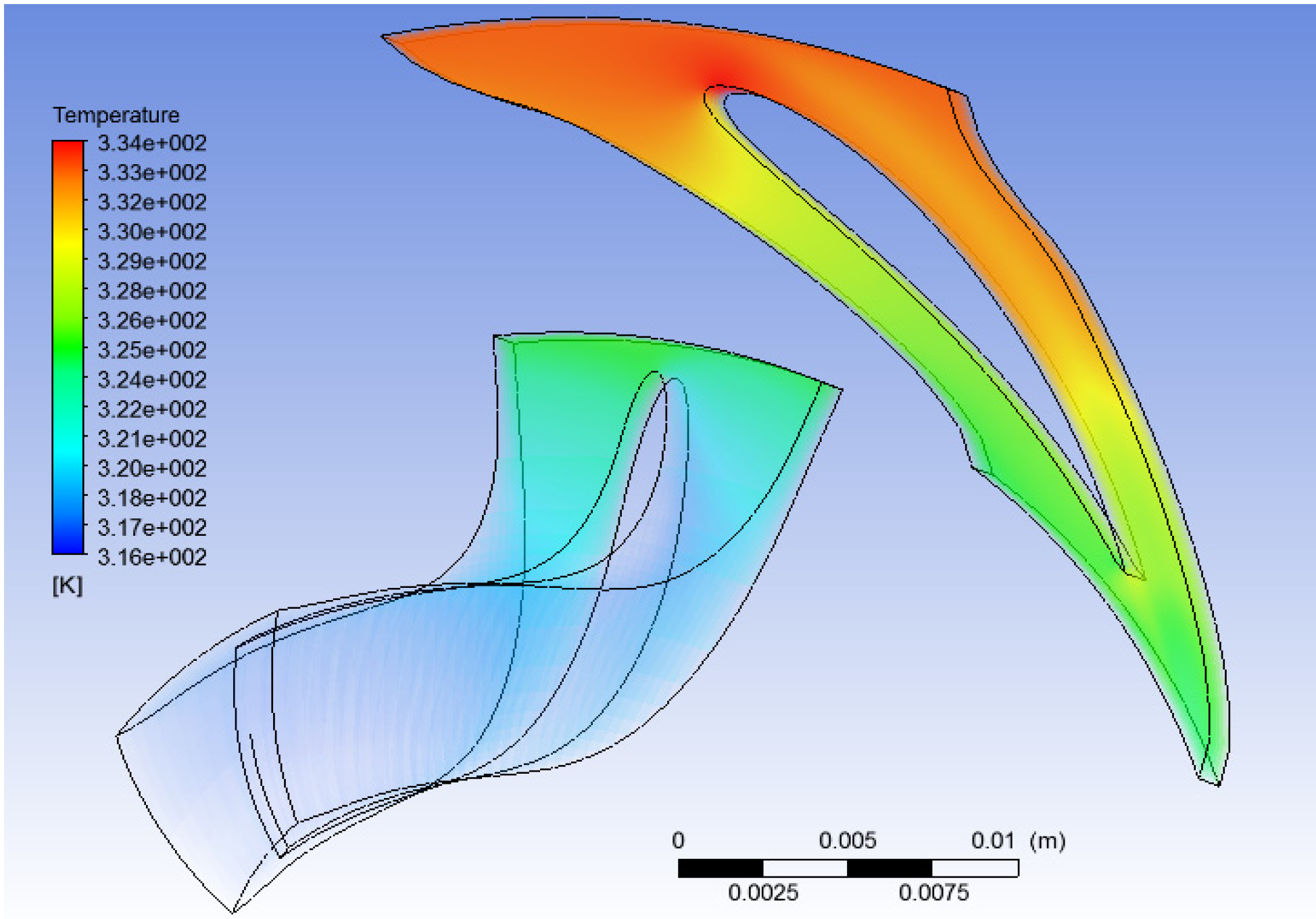
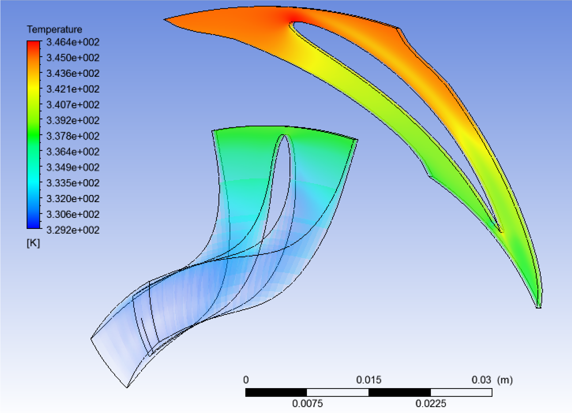
High-pressure bubbles can be noted on the stator leading edge due to the flow impact with the blade (normal behavior) that may (on further studies) cause over-pressure situations on previous components. As well as for the pressure, the temperature behavior in every simulation is smooth with values close to those predicted in theoretical and thermodynamic calculations (Figure 23, Figure 24 and Figure 25).

Figure 23. CFD study results: Temperature (water).

Figure 23. CFD study results: Temperature (water).

Figure 24. CFD study results: Temperature (R134a).

Figure 24. CFD study results: Temperature (R134a).

Figure 25. CFD study results: Temperature (R245fa).

Figure 25. CFD study results: Temperature (R245fa).

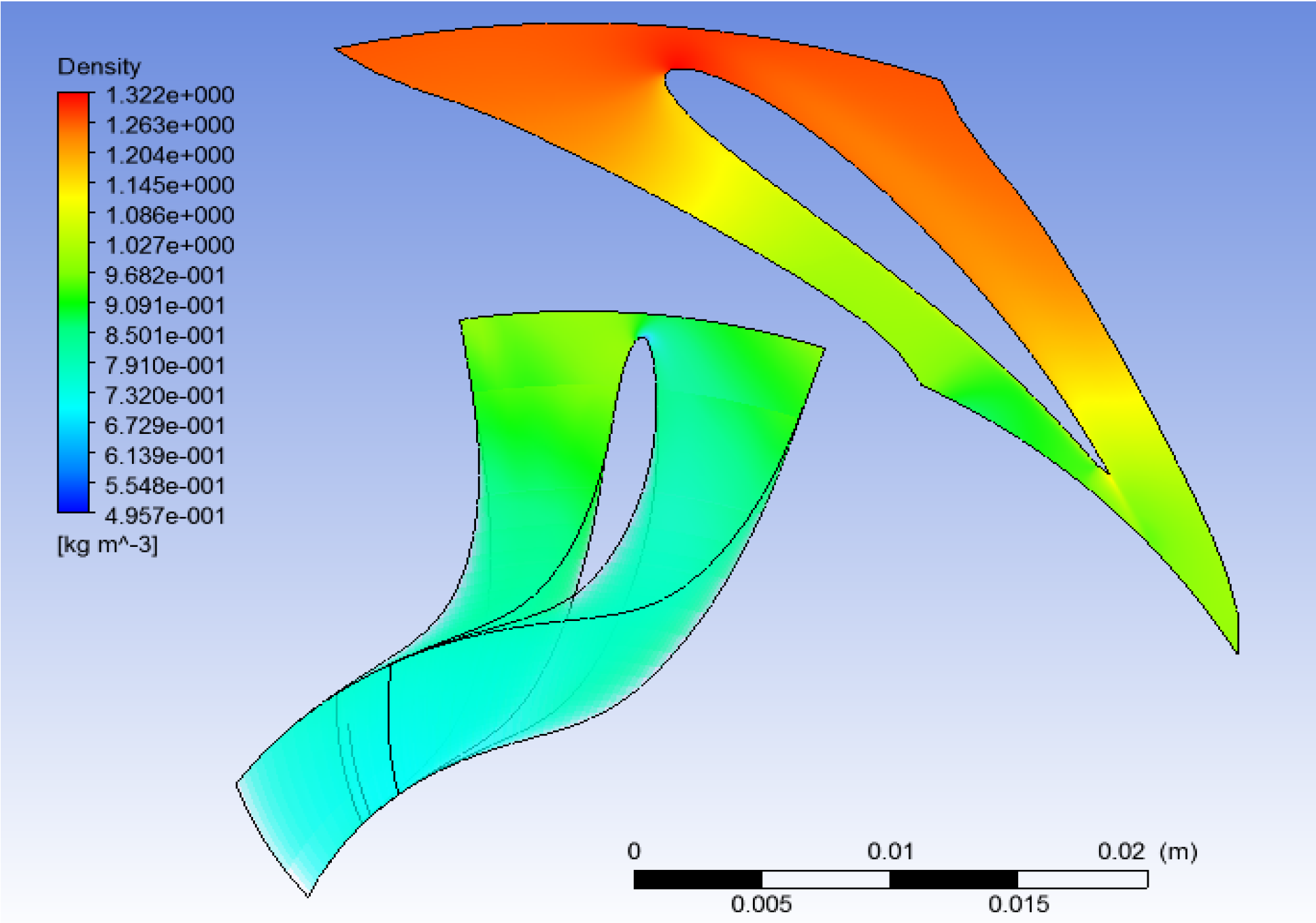
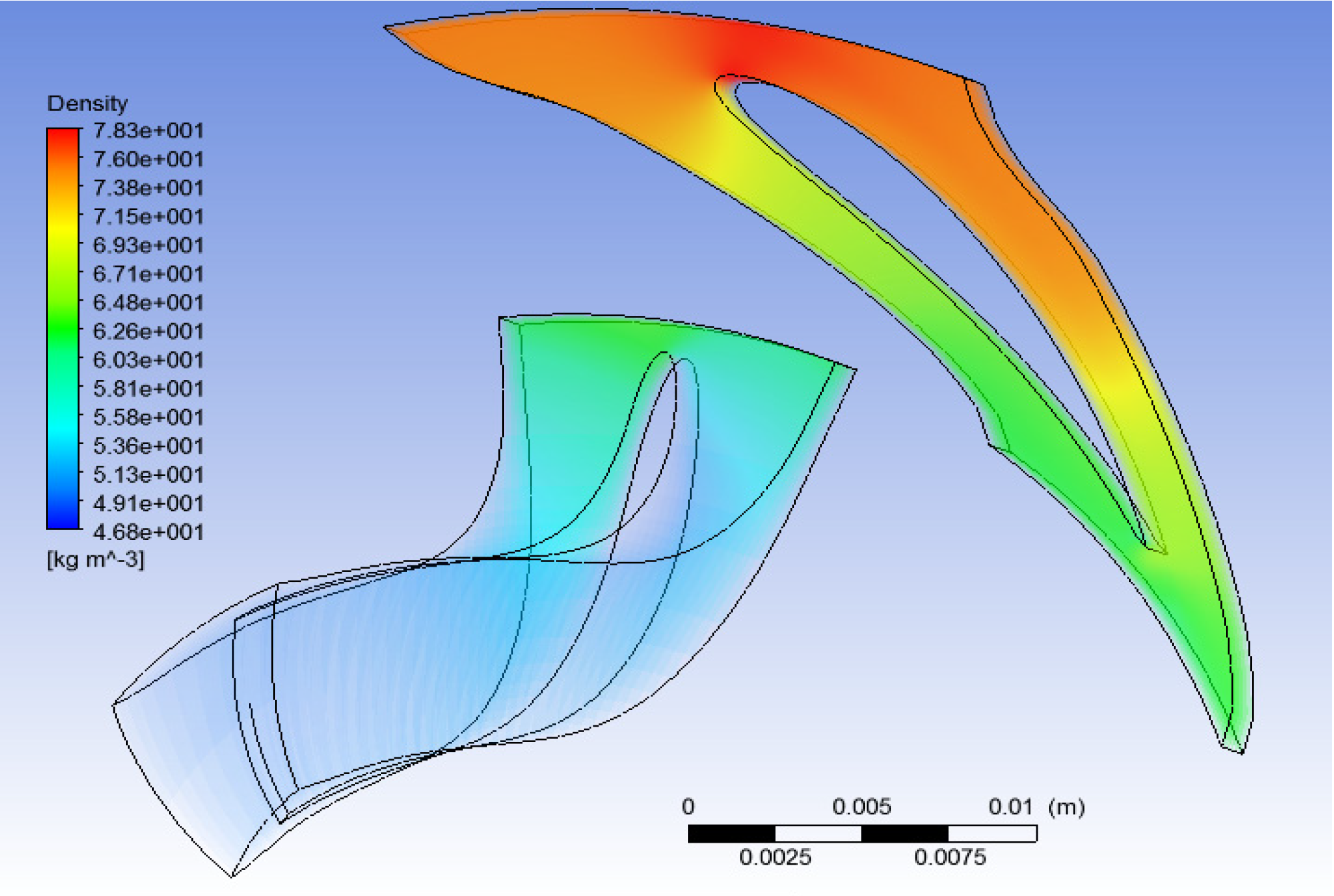
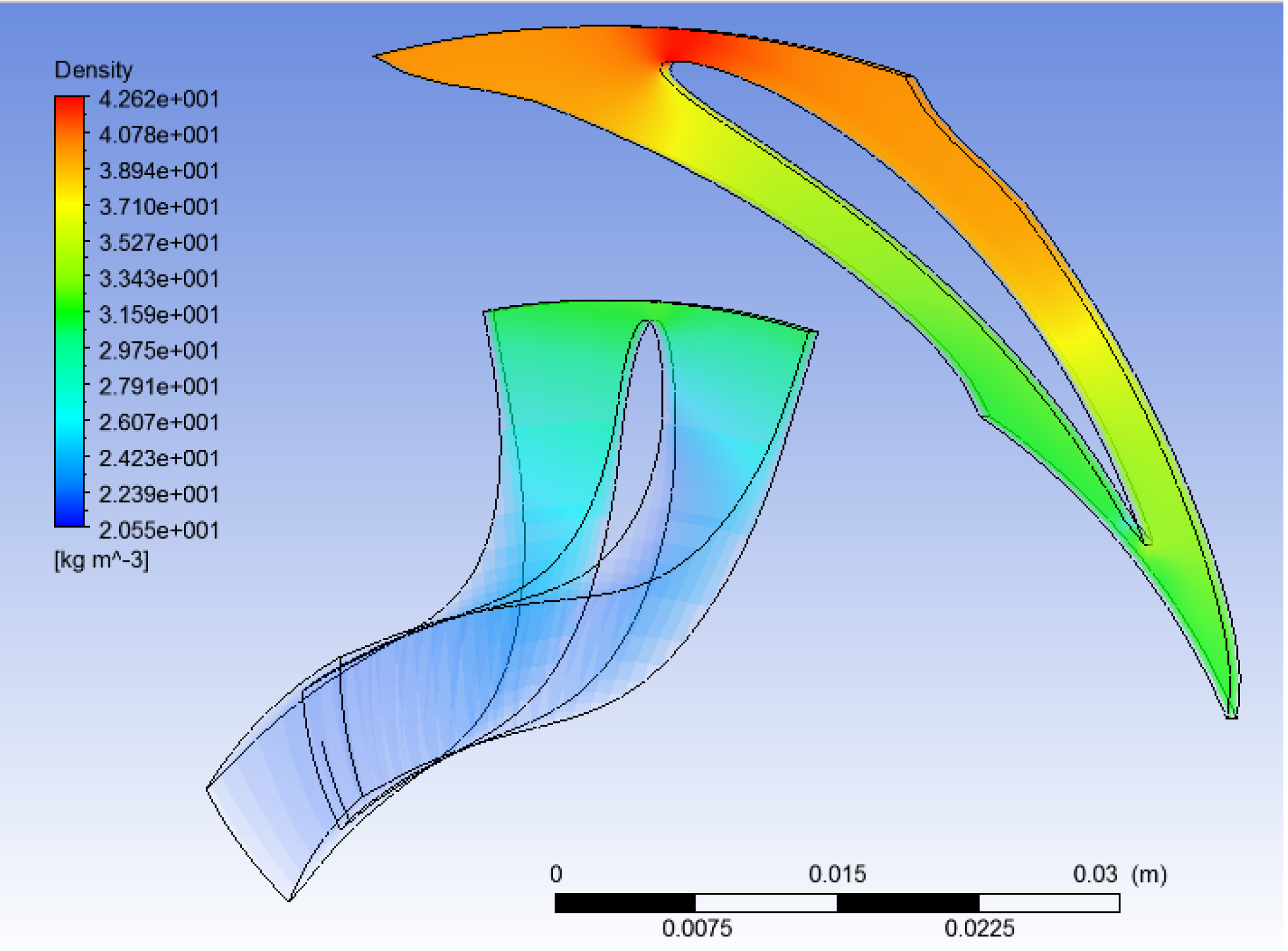
The density values attained through the CFD simulations are slightly different from those computed in the theoretical and thermodynamic calculations, but this variation is probably caused by small differences in the fluid definition between the CFD software and the software used for thermodynamic simulation, or maybe the combination of different pressures and temperatures (commented above) caused the variation in density. However, the values obtained are close enough to consider the simulation valid (Figure 26, Figure 27 and Figure 28).

Figure 26. CFD study results: Density (water).

Figure 26. CFD study results: Density (water).

Figure 27. CFD study results: Density (R134a).

Figure 27. CFD study results: Density (R134a).

Figure 28. CFD study results: Density (R245fa).

Figure 28. CFD study results: Density (R245fa).

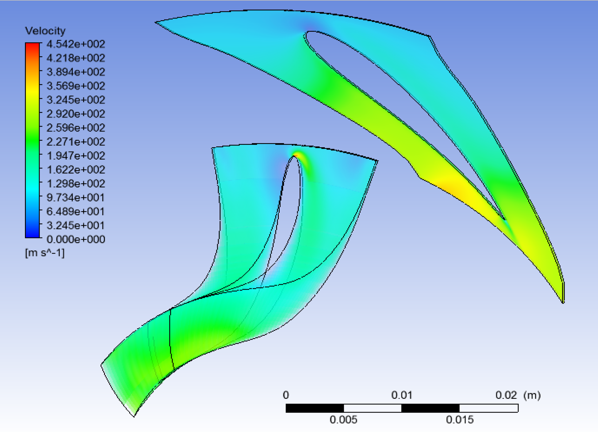
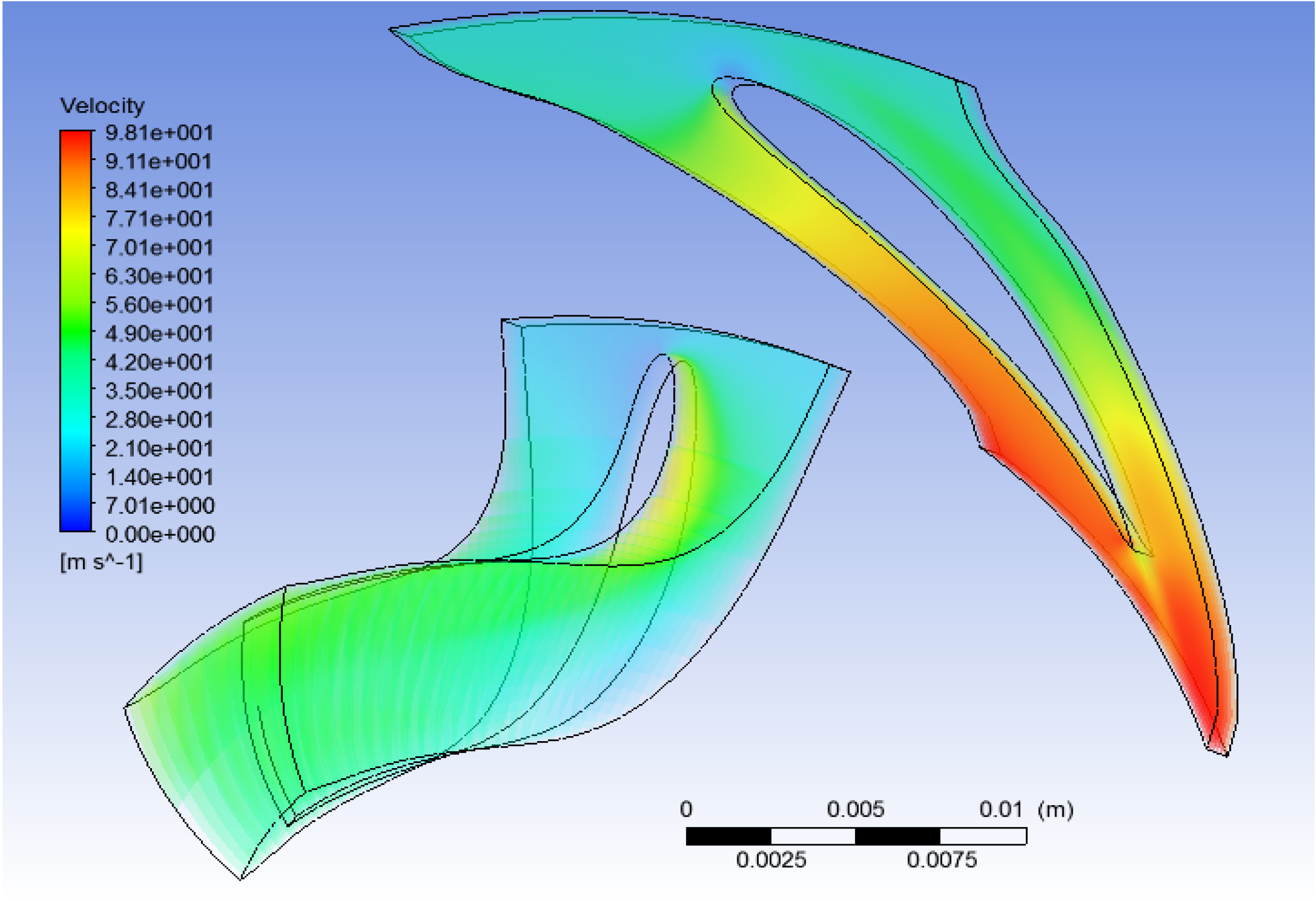
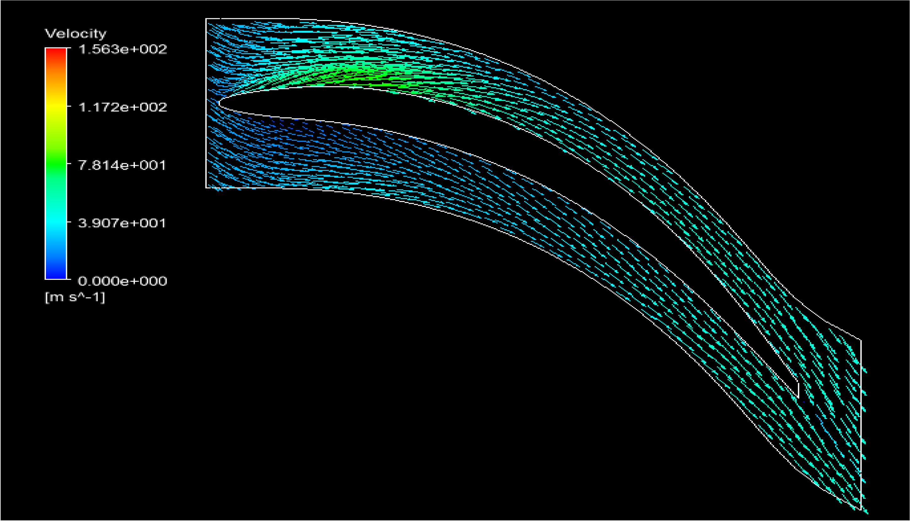
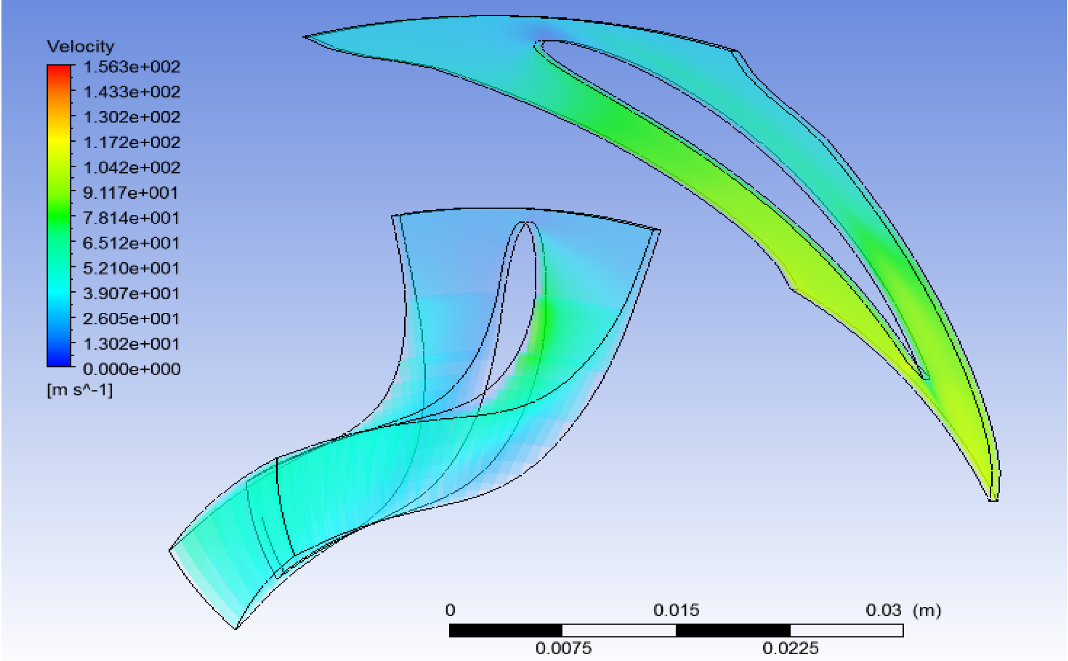
In the velocities field of this study some aspects have to be underlined:

In the stator’s domain we can appreciate the acceleration of the fluid corresponding to the absolute velocity, on the other hand, we can also appreciate the acceleration of the flow in the impeller’s domain, but this time corresponding to the relative velocity (Figure 29, Figure 30 and Figure 31).

Figure 29. CFD study results: Velocity volume (Water).

Figure 29. CFD study results: Velocity volume (Water).

Figure 30. CFD study results: Velocity rendering volume rendering (R134).

Figure 30. CFD study results: Velocity rendering volume rendering (R134).

Figure 31. CFD study results: Velocity volume rendering (R245fa).

Figure 31. CFD study results: Velocity volume rendering (R245fa).

In all cases, it can notice the normal behavior of the fluid passing through an impeller, which is a low velocity flow in the pressure section of the blade and a high velocity flow on the suction section of the blade.

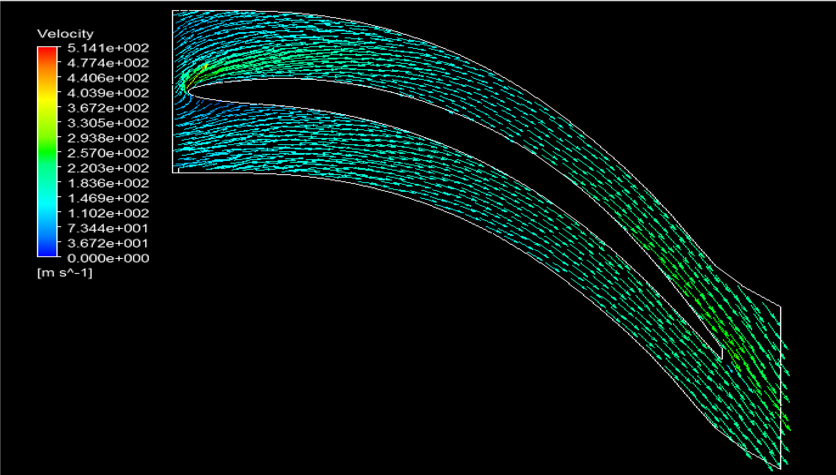
In the case of simulations with R-245fa (Figure 32) the flow at the inlet of impeller is not “purely” radial, as assumed in the theoretical calculations, but this fact does not influence the performance of the rest of the impeller.

At the outlet of the impeller, the relative velocity direction is respected in every case, but, for water and R-245fa there is a difference in the magnitude of the respective velocities between the theoretical and simulations results (Figure 33).

In the simulation with R-245fa, the velocity at the outlet of the nozzle is slightly lower than the one obtained from theoretical calculations; this could be causing the deviation from the radial direction at the impeller’s inlet. There is a region in the blade leading edge, where the pressure decreases and the velocity increases causing the formation of a vortex that can influence negatively the performance of the turbine. This situation indicates that further study to improve the profile of the blade is necessary.

Figure 32. CFD study results: Velocity mid-spam detail (R-245fa).

Figure 32. CFD study results: Velocity mid-spam detail (R-245fa).

Figure 33. CFD study results: Velocity mid-spam detail (Water).

Figure 33. CFD study results: Velocity mid-spam detail (Water).

10. Conclusions

The objective of this work, as mentioned before, was to verify the feasibility of the system and to study the opportunity to make a turbo-expander for these low power rating (2–15 kW). The authors would like to emphasize this, precisely, is the “peculiaritys” of their work: study and submit a design for a small turbo expander for ORC systems. This analysis was divided into several stages:

A preliminary simulation of the ORC system performance by the PRO/II^® software, varying the main operative parameters and considering the R-134a, R245fa and water as working fluids, has been carried out.

The design procedure of the radial expander has been completed under a set of specifications, derived from the previous simulations. In this procedure many other constraints have been added, always keeping in mind the main goal of the project: realize a compact waste energy recovery system, using an “ad hoc” studied and design turbo expander. Finally, the main preliminary geometrical characteristics have been calculated, and a preliminary 3D geometry has been created.

Next, a thermo-structural analysis has been performed, using FEM methods. The analysis suggests adopting a material and verifying, for this specific step of the design procedure, the structural resistance of the impeller.

Then, a CFD study has been performed for each designed turbine. The main objective of these studies was to verify the general performance of the adopted geometries, and to determine if the pressures, temperatures, densities and velocities assumed and obtained by the procedure, match the “real” ones. The result of these CFD studies were shown and discussed.

Once all simulations and expander design are completed, the final step will be to build a prototype and test it. As a final comment, a comparison between the different studied cases has been performed. First, the smallest turbine is obtained when the working fluid is R134a with a net power that is in the middle of the three options; on the other hand, the case that gives the greatest amount of power is when the R245fa is used as working fluid, but this is also the option with the largest turbine.