Article

A Model Predictive Control Approach for Fuel Economy Improvement of a Series Hydraulic Hybrid Vehicle

Department of Mechanical and Automation Engineering, Da-yeh University, 168 University Road, Dacun, Changhua 51591, Taiwan
*
Author to whom correspondence should be addressed.
These authors contributed equally to this work.
Energies 2014, 7(11), 7017-7040; https://doi.org/10.3390/en7117017
Submission received: 1 September 2014 / Revised: 24 October 2014 / Accepted: 28 October 2014 / Published: 31 October 2014

Abstract

:
This study applied a model predictive control (MPC) framework to solve the cruising control problem of a series hydraulic hybrid vehicle (SHHV). The controller not only regulates vehicle velocity, but also engine torque, engine speed, and accumulator pressure to their corresponding reference values. At each time step, a quadratic programming problem is solved within a predictive horizon to obtain the optimal control inputs. The objective is to minimize the output error. This approach ensures that the components operate at high efficiency thereby improving the total efficiency of the system. The proposed SHHV control system was evaluated under urban and highway driving conditions. By handling constraints and input-output interactions, the MPC-based control system ensures that the system operates safely and efficiently. The fuel economy of the proposed control scheme shows a noticeable improvement in comparison with the PID-based system, in which three Proportional-Integral-Derivative (PID) controllers are used for cruising control.

1. Introduction

Forecasted fossil fuel depletion and growing environmental concern have stimulated the development of vehicles with ever-higher efficiency. By combining a renewable energy storage mechanism within the conventional powertrain, hybrid vehicles achieve a significant improvement in fuel economy. The gains are expected from the increasing efficiency of component operations, the utilizing of regenerative braking energy, and the optimizing of engine operation.
In the context of longitudinal dynamics of vehicles, accelerating rate, grade-ability, and maximum vehicle velocity are typical performance criteria. With the purpose of evaluating fuel economy improvement, velocity tracking is the main performance criterion of hybrid vehicles. In conventional vehicles, velocity relates directly to engine speed through a rigid mechanical transmission system. Driving power relates to engine power in the same fashion. A typical cruising control system uses a standard Proportional-Integral/Proportional-Integral-Derivative (PI/PID) controller to estimate the desired throttle opening of the engine. Thus, cruising control of a conventional vehicle is a single-input-single-output control problem.
As a short- and mid-term solution, hybrid vehicles have aroused the attention of researchers and manufacturers all over the world. In the recent past, most commercialization efforts have focused on hybrid electric vehicles (HEVs). Several commercially available HEVs are passenger cars and light truck applications [1]. Recent studies have indicated that hydraulic hybrid vehicles (HHVs) produce further advantages associated with the higher efficiencies of component operations and regenerative braking. Modern hydraulic pumps and motors have higher power density than their electric counterparts. Thus, a compact configuration of HHV can be achieved. In addition, hydraulic accumulators have the ability to operate at high frequencies and high rate of charging and discharging but a relatively low energy density in comparison with electro-chemical batteries. The relative low energy density of the hydraulic accumulator should be considered and required a carefully designed control strategy if the fuel economy potential is to be realized.
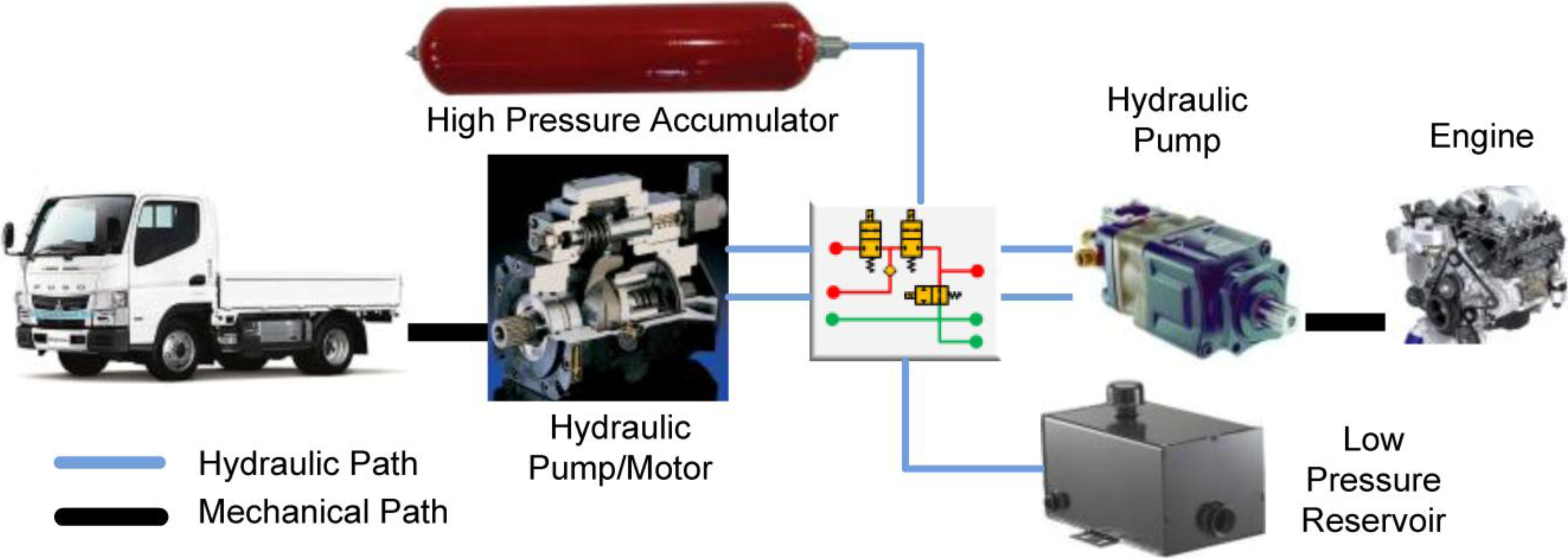
In a series hydraulic hybrid vehicle (SHHV), a hydrostatic transmission is used instead of a conventional mechanical transmission. Integrated hydraulic accumulator works as an on-board energy storage device in addition to the conventional engine. Therefore, a power demand can be satisfied by combining the two power sources in different manner. The power can be supplied by only the engine, only the accumulator, or both simultaneously. In addition, by decoupling the engine from the wheels, the series hydraulic hybrid architecture adds more degree-of-freedom to engine control. In this scenario, engine torque, engine speed, and accumulator pressure are control variables in addition to vehicle velocity. Due to physical constraints and input-output interactions, cruising control in an SHHV remains a challenge for standard PI/PID controllers.
Several approaches have been developed for cruising control in HHVs. A fuzzy logic controller (FLC) was developed by Matheson and Stecki [2] for use in the parallel HHV. For a given power demand from drivers, the FLC determined the most suitable operating points of the engine corresponding to current states system. However, the resulting control law cannot be implemented in real-time system because ADVISOR is a backward-facing simulation.
In [3], Wu et al. divided the engine operating range into three zones by two constant-power lines: a low- and a high-power limit. This rule-based power management strategy improves fuel economy by forcing the engine to operate at higher efficiency. The optimal gearshift logic was achieved by applying dynamic programming (DP) technique. The DP results were extracted for use in improving the initial rule-based control strategy to achieve further improvement in fuel economy. However, how to regulate the engine to its reference power was not presented in this study. Similar problems were found in [4,5,6].
In [7], engine speed is controlled using a PI controller, which uses vehicle velocity error as the input. Engine torque is controlled by adjusting the control signal of the fuel rack. Control of vehicle velocity is not discussed explicitly in this study. In [1], engine speed and vehicle velocity are controlled by individual PID controllers. Similarly, in [8], three individual PID controllers are used to control engine torque, engine speed, and vehicle velocity to track to the corresponding references. Controller parameter tuning, input-output interaction and physical constraint are obstacles to this control approach.
With the capability of applying constraints on both state and control inputs, model predictive control (MPC) is a widely recognized control methodology for complex systems. The controller estimates a future control trajectory that minimizes the quadratic cost function, which reflects the optimization goals, and is subject to the dynamic constraints of the system over a finite prediction horizon. Recently, MPC has been applied to solve the optimal control problem in power-split HEVs [9,10,11], and in HHVs [12,13].
Deppen et al. developed MPC-based energy management for a parallel HHV [12] and a lightweight passenger SHHV [13]. Engine throttle, pump displacement, and valve opening are the input variables. The optimal input is obtained by solving the optimal control, in which the objective function is to minimize the velocity tracking error and ensure that the actuators operate efficiently. Ignoring braking energy regeneration, limiting the engine to operate with constant torque and speed are restraints associated with these work.
This study presents a systematic illustration of a controller for the tracking problem in a hydraulic hybrid powertrain system using a linear MPC methodology. The remainder of this paper is divided into four sections. 
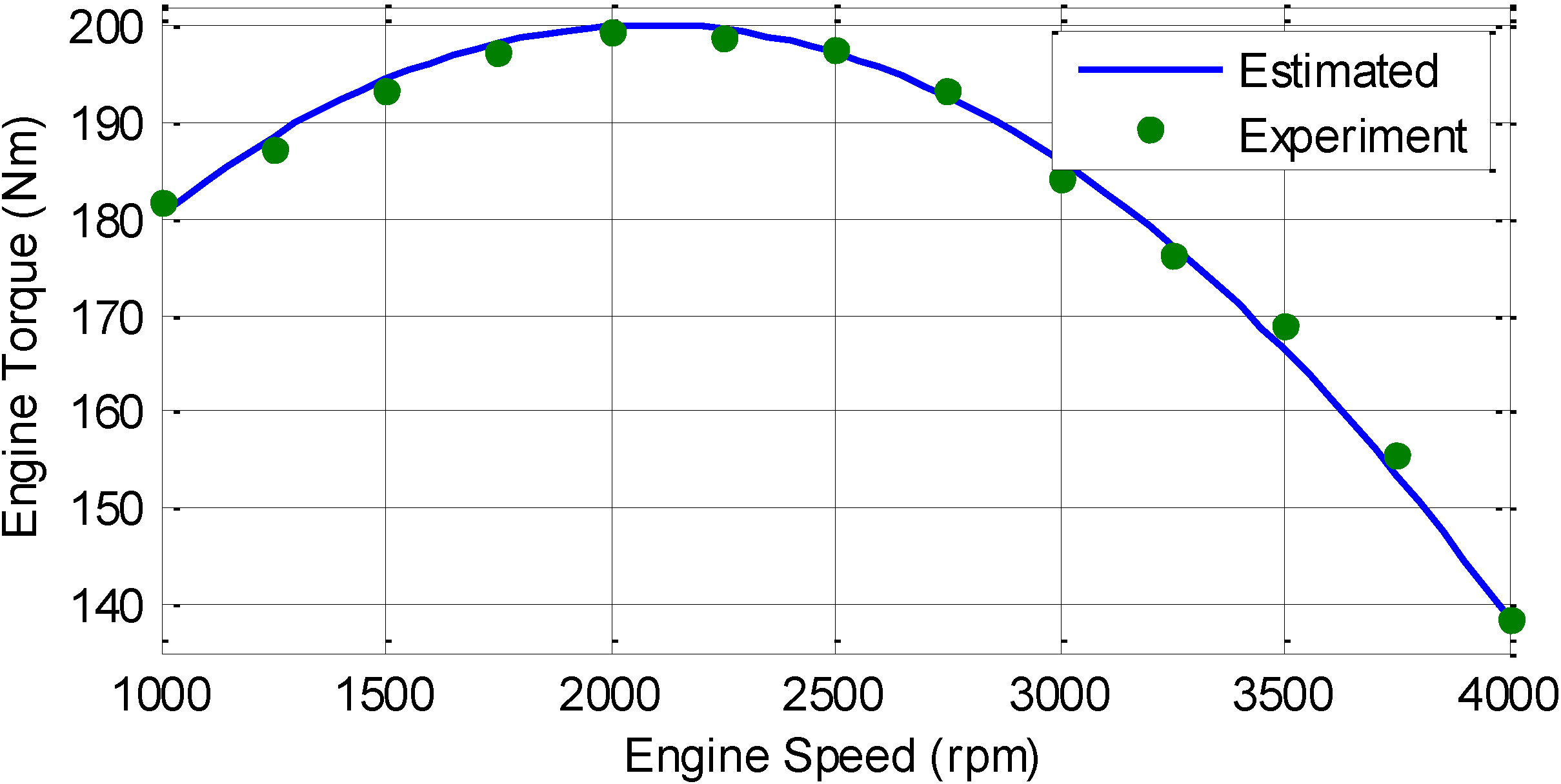
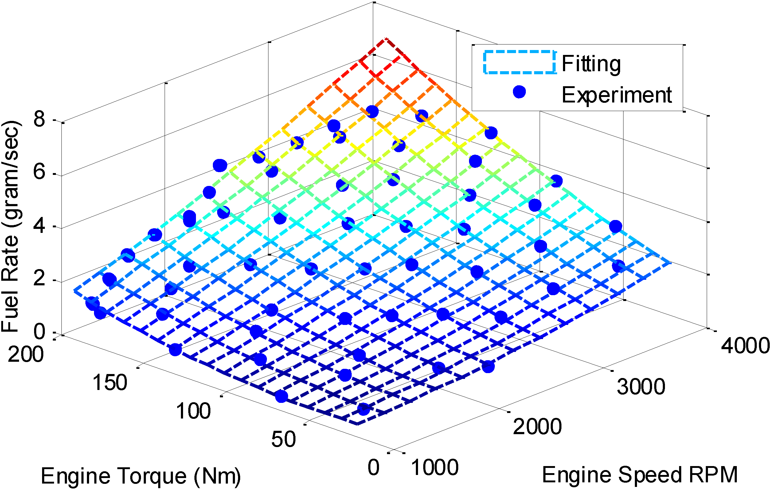
Section 2 describes the modeling configuration of the series hydraulic hybrid powertrain system. A high-fidelity nonlinear model of the SHHV was established in MATLAB/Simulink. This model is used as the plant in the simulation. In addition, a control-oriented model for the design of MPC was also derived in this section.
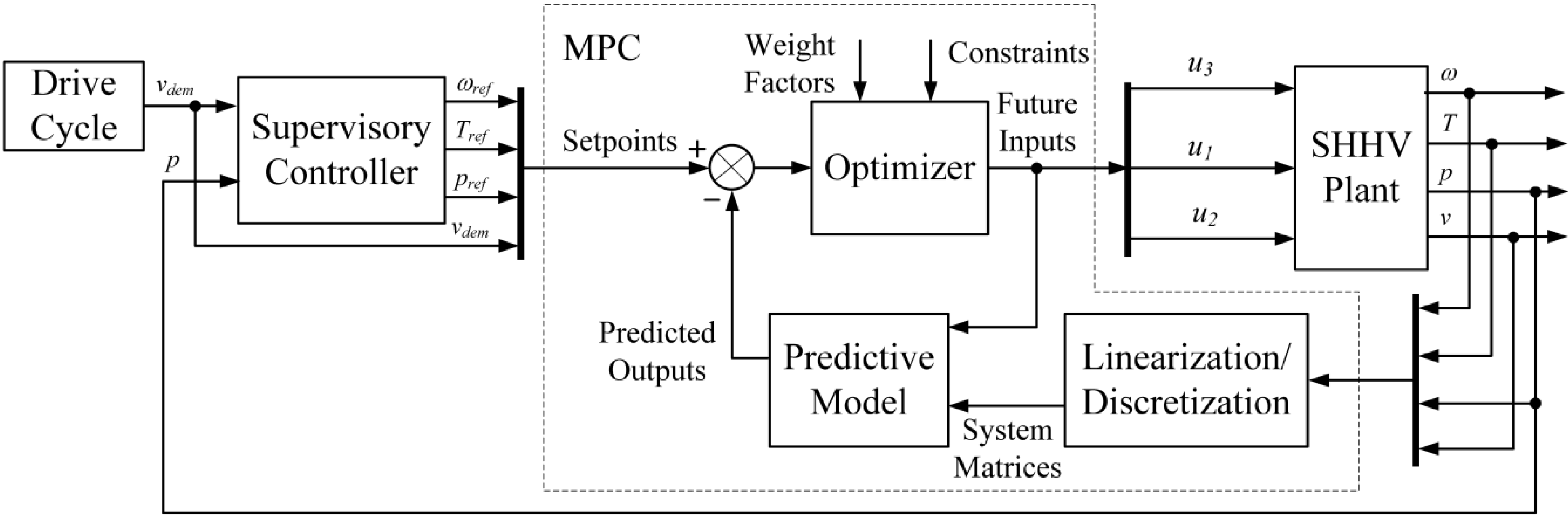
In Section 3, the MPC-based control system is presented. The supervisory controller determines optimal reference values for engine speed, engine torque, and accumulator pressure to satisfy the demand for a given vehicle velocity. The MPC regulates the engine, the variable displacement pump, and the pump/motor to ensure that vehicle velocity, engine speed, engine torque, and accumulator pressure adhere to their corresponding reference values. At each time step, the MPC algorithm uses a linearized model to predict future output. A quadratic programming problem is then solved resulting optimal input vector, which minimizes the objective function with respect to physical and dynamic constraints. The objective function includes the penalty on the output tracking error and the rate of change of the control input. The effect of various output-weighting factors on system outputs is also investigated in this section.
Simulation and results are presented in Section 4. The proposed MPC-based control scheme was evaluated under urban and highway driving conditions using Japan 1015 and Highway fuel economy test (HWFET) drive cycles. The proposed control scheme shows noticeable improvements over the PID-based control scheme. In Section 5, important conclusions and further directions of study are discussed.

2. System Configuration and Modeling

2.1. System Description

A schematic of the SHHV is presented in Figure 1. In this configuration, conventional mechanical transmission is eliminated. A variable displacement hydraulic pump is connected to an engine to convert mechanical power into hydraulic power. The power is stored in the accumulator or converted back to mechanical power by a variable displacement pump/motor. The pump/motor is a reversible energy conversion component. When working as a motor, it converts the hydraulic power into mechanical power to propel the wheels. When the brakes are applied, the pump/motor works as a pump. In this manner, mechanical brake power is converted into hydraulic power. The braking energy is captured and stored in the accumulator in the form of hydraulic pressure. The low-pressure reservoir provides fluid for the hydraulic system.
Figure 1. Schematic of a series hydraulic hybrid vehicle.
Energies 07 07017 g001

2.2. Detailed Model of SHHV

To deal with closed-loop simulations, this study established a detailed model of an SHHV using the SimscapeTM toolbox in MATLAB/Simulink. The toolbox provides environment for modeling and simulating multi-domain physical systems, including mechanical, hydraulic, and automotive drivelines [14]. The model composed of one diesel engine block, one variable displacement pump block, one pump/motor block, one vehicle body block, four tire blocks, one differential block, two gas-charged accumulator blocks, and a number of pipeline blocks. Most of these blocks are datasheet-based models, which allow for customization of the component parameters according to experiment and manufacturer data. More details of the modeling procedure can be found in [15]. This high-fidelity dynamics model of the SHHV was selected as the plant of the SHHV for simulation in this study.

2.3. Simplified Model of SHHV

The complexity of the SHHV Simulink model made it difficult to apply in control design. In this section, we outline a simplified control-oriented model that captures the key features essential to the development of the control system. The engine simulation model is based on the experimental data, which was obtained at the Automotive Research and Testing Center, Taiwan. The corresponding brake specific fuel consumption map (BSFC) of the engine is shown in Figure 2.
Figure 2. Experimental brake specific fuel consumption map of the engine.
Energies 07 07017 g002
The attainable torque of an internal combustion engine is a function of the engine angular speed and the fuel mass in the cylinders as below:
T e ( ω e ) = u 3 T e , max ( ω e )
where u3 is the normalized fuel mass, in the cylinders, u3 equals to zero indicated that there is no fuel in cylinders and u3 equals to one means that maximum allowable fuel mass was injected into cylinders. In this case, the engine delivers its maximum available torque, which is considered as a function of the angular speed only.
The maximum available torque of the engine at a steady state angular speed ωe, was derived from the engine map approximately by the second-order polynomial as:
T e , max ( ω e ) = k 1 + k 2 ω e + k 3 ω e 2
where k1 = 127.3, k2 = 0.6677, k3 = −0.0015 are fitting coefficients.
In the SHHV configuration, the engine is connected directly to the hydraulic pump. The dynamics of the engine is:
ω ˙ = 1 J e + J P1 ( T e T 1 )
where T1 is the load torque of the pump which is connected to the engine, and Je and JP1 are the engine and pump inertia, respectively.
Based on the empirical engine map, the fuel flow rate is related to the engine speed and engine torque by following expression:
m ˙ f = k 00 + k 10 ω e + k 20 ω e 2 + k 11 ω e T e + k 01 T e + k 02 T e 2
where the fitting coefficients are listed in Table 1. The fitted and the experiment data are closed together as represented in Figure 3 and Figure 4.
Table 1. Fitting coefficients.
CoefficientValue
k000.7213
k10−0.002796
k201.157 × 10−5
k116.52 × 10−5
k01−0.01162
k025.931 × 10−5
Figure 3. Maximum available torque of the engine.
Energies 07 07017 g003
Figure 4. Fuel consumption rate of the engine.
Energies 07 07017 g004
In this work, the same model has been used for both the pump and the pump/motor. The only difference is the range of their displacements. The displacement of the pump is always positive while the displacement of the pump/motor is positive when it works as a motor and negative when it works as a pump. The actual torque and flow rate of hydraulic pump/motor are determined by below expression, using the updated Wilson’s theory [16]:
T 1 , 2 = u 1 , 2 D 1 , 2 Δ p 1 , 2 η t 1 , 2
q 1 , 2 = u 1 , 2 D 1 , 2 ω 1 , 2 η v 1 , 2
where u1,2 are the normalized displacements, D1,2 are the maximum volumetric displacement, ∆p1,2 are the pressure different, and ω1,2 are the angular speed of the pump and pump/motor, respectively. The mechanical torque efficiency ηt1,2 and volumetric efficiency ηv1,2 of the pump and pump/motor depend on leakage, shaft friction, current displacement, pressure across, and angular speed as represented below:
η v = { η v,P = f ( k L1 , x , ω , Δ p )    for pump mode 1 2 η v,P                          for motor mode
η t = { η t,P = f ( k F1 , x , ω , Δ p )      for pump mode 2 1 η t,P                              for motor mode
where kL1 and kF1 are the leakage and friction proportionality coefficients of the pump, respectively.
For the hydraulic accumulator, energy conservation is applied to the nitrogen gas being compressed by the hydraulic fluid. Disregarding the compression of fluid, and assuming nitrogen is an ideal gas the relationship between the flow rate and the pressure of the fluid in the accumulator can be expressed as follows:
q a = { V a p pr 1 / 1.4 1.4 p 2.4 / 1.4 p ˙   when    p p pr 0                   when   p < p pr
where Va is the capacitor, ppr is the gas pre-charged pressure and p is the fluid pressure at the inlet port of the accumulator, respectively.
The hydraulic transmission hose carries fluid throughout the system. The direction of flows within the high-pressure hose of the SHHV system is presented in Figure 5. The one-way arrow indicates that the pump delivers fluid for the system. The two-way arrow indicates that the accumulator can absorb or deliver fluid. The direction of fluid flowing through the pump/motor depends on the working mode of this component. The dynamic of the fluid pressure at the junction can be expressed using following equation:
p ˙ = β V h ( q 1 q a q 2 )
where β is the fluid bulk modulus, Vh is the volume of the hose, and q1, qa, and q2 are the flow rates of the pump, the accumulator, and the pump/motor , respectively.
Figure 5. Flow directions within the high-pressure hose of the SHHV.
Energies 07 07017 g005
Substituting Equations (6) and (9) into Equation (10) and rearranging the terms gives the following results:
p ˙ = 1.4 β ( 1.4 V h + β V a p pr 1 / 1.4 p h 2.4 / 1.4 ) ( u 1 D 1 ω e u 2 D 2 v i df r w )
Disregarding inertial loss of the differential gearbox, the kinetic equality constraints between the pump/motor and the vehicle wheel are as follows:
T 2 = T w i df ω 2 = v r w i df
where idf is the differential gear ratio, rw is the wheel radius, T2 and ω2 are the torque and the speed at the output shaft of the pump/motor, respectively, Tw and v are the driving torque and the vehicle velocity, respectively. The vehicle is assumed a dump mass model, and its velocity dynamic is as follows:
v ˙ = 1 m ( T w T brk r w 1 2 ρ C d A v 2 m g f r cos ( θ ) m g sin ( θ ) )
where Cd and ρ drag coefficient and air density, m and Af are the mass and frontal area of the vehicle, θ is the road grade, and g is the gravity acceleration.
In Equation (13), Tbrk is the mechanical braking torque delivered from the mechanical brake system, which is used in addition to the regenerative braking system. With the purpose of recovering the brake energy as much as possible, the conventional brake system is involved only for emergencies. Assuming that the regenerative braking system can afford any desired braking torque within a given driving test schedule, Tbrk is eliminated from the vehicle dynamics in the oriented-control model. In practical systems, fluid pressure in the hydraulic hose is normally higher or at least equal to atmospheric pressure. However, preventing the depletion of pressure in the accumulator when the vehicle is on the road requires that the fluid pressure in the high-pressure hose is considerably higher than the pre-charged pressure of the accumulator. For system safety, the pressure in the accumulator is limited by minimum and maximum thresholds. Engine speed, engine torque, and vehicle velocity are also limited by physical constraints:
p min p p max ω min ω e ω max 0 T e ( ω e ) T e, max ( ω e ) 0 v v max
In short, the dynamics of the SHHV can be represented using the following equations:
ω ˙ = 1 J e + J P1 ( u 3 ( k 1 + k 2 ω e + k 3 ω e 2 ) u 1 D 1 p ) p ˙ = 1.4 β ( 1.4 V h + β V A1 p pr,A1 1 / 1.4 p h 2.4 / 1.4 ) ( u 1 D 1 ω e u 2 D 2 v i df r w ) v ˙ = 1 m ( u 2 D 2 p i df r w 1 2 ρ C d A v 2 m g f r cos ( θ ) m g sin ( θ ) )
They can also be represented in vector form:
x ˙ = f ( x , u , t ) y = g ( x , u , t )
where the state vector x = [ ω e   p   v ] T , the measured output vector y m = [ ω e p v T e m ˙ f ] , the controlled output vector y r = [ ω e T e p v ] , and the input vector u = [ u 1 u 2 u 3 ] T . The components of the input vector are the normalized factors of the injected fuel mass of the engine, and the displacement of the pump and pump/motor, respectively. The input is constrained as follow:
[ 0 0 1 ] T u [ 1 1 1 ] T
Using a general Matlab S-function template, we created a model of the SHHV with four control inputs, three states, and five outputs. The compiled code in the function is then inserted into a special “S-function” block, which can be used as standard block in Simulink. The parameters of the system are listed in Table 2.
Table 2. System parameters.
SymbolParameterValue
mMass (Gross Weight)3490 kg
AfFront Area2.5 m2
CdDrag Coefficient0.3
ρAir Density1.2 kg·m−3
idfDifferential Ratio4.875
frRolling Resistance0.008
rwTire radius0.312 m
θRoad grade0%
Pe,maxMaximum Output Power of the engine61 kW
ωe,maxMaximum Engine Speed4700 rpm
ωe,minMinimum Engine Speed200 rpm
JeEngine inertia0.12 kg·m2
JP1Pump inertia0.02 kg·m2
D1Maximum displacement of the pump55 cm3·rev−1
D2Maximum displacement of the pump/motor75 cm3·rev−1
VaAccumulator Capacitor68 L
VhHigh-pressure hose volume1.85 L
pa,maxMaximum working pressure of the accumulator350 bar
pprPre-charge Pressure of the accumulator120 bar

2.4. Model Validation

In this simulation, the two models of the SHHV are simulated using the control inputs shown in Figure 6a. System behavior is represented in Figure 6b. This test illustrates a common driving pattern: a start-stop-and-go. During the first 20 s, the engine propels the wheel and charges the accumulator. After that, the engine is deactivated and only the accumulator propels the vehicle. At 30 s, the pump/motor switches from motor to pump mode, whereupon the vehicle decelerates to a full stop by 56.5 s. During this period, the accumulator pressure is increased due to regenerative braking. Between 56.5 and 72 s, captured energy is used to accelerate the vehicle again. To prevent depletion of pressure in the accumulator, the engine is engaged once again, whereupon the vehicle runs in cruising mode.
Figure 6. SHHV models validation. (a) Control inputs; and (b) System outputs.
Energies 07 07017 g006aEnergies 07 07017 g006b
The result indicates that the simplified model captures the time scales and approximate magnitudes of each system output throughout the test. Larger differences were observed in the engine speed when the engine was deactivated. However, for all outputs, the relative differences were within 10% throughout the test. Thus, the simplified model was deemed sufficient for control analysis and design.

3. Control System Design

In the standard cruising control systems available on conventional vehicles, the throttle and brakes are the actuators to regulate the velocity. In the SHHV system, the cruising control not only regulates the vehicle velocity but also engine torque, engine speed, and accumulator pressure. In this work, a discrete MPC was applied to estimate the control signals for the engine, the pump, and the pump/motor. A schematic diagram showing an MPC-based control system is presented in Figure 7. To achieve a desired velocity, the supervisor uses the current pressure of the accumulator as a feedback variable to calculate the desired values for engine speed, engine torque, and accumulator pressure. At each time step, the SHHV plant is linearized around its current inputs and outputs and is discretized to obtain a linear and discrete model. The model is used to estimate the outputs within a receding horizon. The optimizer solves a quadratic programming problem to estimate the optimal input sequence, of which the first element is applied to the plant. The following sections provide details related to the important components in the MPC-based control system.
Figure 7. Schematic of the MPC-based control system.
Energies 07 07017 g007

3.1. Supervisor

This control scheme was initially developed by Kim in [7], in which it was termed a modulated State-Of-Charge (SOC) control scheme. It was further developed by Tavares et al. in [17], in which it was referred to as a hydrostatic control strategy. The purpose of this control strategy is to maintain the pressure in accumulator at a constant level in order to prevent the engine from charging the accumulator unnecessarily. A well-chosen value for the reference pressure can help to improve the efficiency regenerative braking. However, when pressure in the accumulator is maintained at a constant level, the engine power is related directly to wheel load, which reduces the flexibility in controlling the engine. If the constant pressure is set too low, excessive vehicle power demand will necessitate a larger displacement hydraulic pump/motor. If pressure is set too high, the available volume for storing brake energy will be reduced.
A schematic diagram showing the supervisory controller is presented in Figure 8. In this case, the reference value for accumulator pressure is considered a function of the current vehicle velocity. The idea of this approach originates from the fact that when the vehicle velocity is low, the engine can charge the pressure to a high-pressure level in preparation for higher demand power. A higher vehicle velocity would require that the pressure in the accumulator be low in order to reserve sufficient accumulator volume to enable the storage of braking energy. The PI controller uses the difference between pressure in the accumulator and its corresponding reference value to determine the power demand of the engine. Details related to the estimation of the optimal reference values for a given demand of vehicle velocity are presented in the following.
Figure 8. Schematic of the Supervisory Controller.
Energies 07 07017 g008
The amount of energy that an accumulator can store when charging from a reference pressure to its maximum pressure can be approximated as follows:
E acc = V a p pr 5/7 0.4 [ p max 2 / 7 p ref 2 / 7 ]
where pmax is the maximum working pressure and pref is the reference pressure of the accumulator, respectively.
Assuming the vehicle is demanded to reach the velocity of vdem, and disregarding the effect of rolling resistance and air drag, the maximum kinetic energy that the system can recover from a full-stop brake is:
E brk = 1 2 m v dem 2
To capture the whole braking energy, we set Eacc = Ebrk. The reference value of pressure in the accumulator is obtained as follows:
p ref = ( p max 2 / 7 1 5 m v dem 2 V a p pr 5/7 ) 7 / 2
For a given power demand, Pdem, the reference speed of the engine is approximated using a third order polynomial as follows:
ω ref = l 2 ( P dem l 1 ) 3 + l 3 ( P dem l 1 ) 2 + l 4 P dem + l 5
where l1 = 37.75, l2 = 0.0311, l3 = 0.044, l4 = 52.83, and l5 = 387.5 are the fitting coefficients.
The optimal reference torque of the engine is then determined by:
T ref = π 30 1000 P dem ω ref

3.2. Predictive Model

In order to estimate the optimal control input by applying the linear MPC at each time step, the nonlinear model is linearized around the current state x0 and input u0. Using the first derivative term in the Taylor series expansion of Equations (16) for a small variation δx and δu we obtained:
x ˙ = A x + B u y r = C x + D u
where:
A = ( f x ) ( x 0 , u 0 ) = [ a 1 a 2 0 a 3 a 4 a 5 0 a 6 a 7 ] ;               B = ( f u ) ( x 0 , u 0 ) = [ b 1 0 b 2 b 3 b 4 0 0 b 5 0 ] C = [ 1 0 0 c 1 0 0 0 1 0 0 0 1 ] ;                                        D = [ 0 0 0 0 0 d 1 0 0 0 0 0 0 ] ;
in which:
a 1 = u 3 , 0 ( k 2 + 2 k 3 ω e , 0 ) J e + J P1 ;     a 2 = D 1 u 1 , 0 J e + J P1 ;    a 3 = 1.4 β ( 1.4 V h + β V A1 p pr,A1 1 / 1.4 p h , 0 2.4 / 1.4 ) u 1 , 0 D 1 ;   a 4 = 2.4 1.96 β V h V A1 p pr,A1 1 / 1.4 p 0 3.8 / 1.4 ( x 1 , 0 D 1 ω e , 0 x 2 , 0 D 2 v 0 i df r w ) ;   a 5 = u 2 , 0 D 2 i df r w 1.4 β ( 1.4 V h + β V A1 p pr,A1 1 / 1.4 p h , 0 2.4 / 1.4 ) ;       a 6 = 1 m u 2 , 0 D 2 i df r w ;          a 7 = 1 m ρ C d A v 0 ; b 1 = D 1 p 0 J e + J P1 ;        b 2 = k 1 + k 2 ω e , 0 + k 3 ω e , 0 2 J e + J P1 ;           b 3 = 1.4 β ( 1.4 V h + β V A1 p pr,A1 1 / 1.4 p h , 0 2.4 / 1.4 ) D 1 ω e , 0 ; b 4 = D 2 v 0 i d f r w 1.4 β ( 1.4 V h + β V A1 p pr,A1 1 / 1.4 p h , 0 2.4 / 1.4 ) ;           b 5 = 1 m p 0 D 2 i df r w ; c 1 = u 3 , 0 ( k 2 + 2 k 3 ω e , 0 ) ;                                    d 1 = ( k 1 + k 2 ω e , 0 + k 3 ω e , 0 2 )
The linearized continuous model is then discretized using the zero-order-hold method with sampling time τs = 0.1 s to derive a linearized-discrete model. It can be seen from Equation (24) that there is an input-output direct feed-through between the injected fuel mass and the torque of the engine. In order to apply standard MPC algorithm, this relationship is eliminated by introducing a new vector of the controlled output [18]. Then the predictive model of the MPC can be presented in the following standard form:
x ( k + 1 ) = A d x ( k ) + B d u ( k ) y r ( k ) = C d x ( k )

3.3. Optimizer

The objective function is composed of two parts. The first term enforces regulation of the controlled output and the second term penalizes the rate of change of the control input:
J = i = 1 4 j = 0 H p λ i ( y i ( k + j + 1 | k ) r i ( k + j + 1 | k ) ) + p = 1 3 q = 0 H u 1 γ p Δ u p ( k + q | k ) 2
where Hu and Hp are the control and prediction horizon, respectively, y ( k + i | k ) R 4 is the predicted output vector, composing engine speed, engine torque, accumulator pressure, and vehicle velocity, y = [ ω e T e p v ] , and r ( k + i | k ) R 4 is the corresponded reference vector, λi is the weight factor on the output ith, and γp is the weighting factor on the rate of change of the input pth. Since the reference values for engine speed, engine torque, and accumulator pressure are the optimal ones corresponding to a demanded vehicle velocity, the smaller the output errors are, the higher the efficiency of the components will be. Increasing efficiency of the components translates directly into an increase in the efficiency of system as a whole, which subsequently enhances fuel economy. In other words, the objective function maximizes the efficiency of the system.
At each time step, the predictive model is used to estimate the state and the output variables of the system within the receding horizon. The objective of the MPC algorithm is to find a sequence of input increments, Δ U = [ Δ u ( k | k ) , ... , Δ u ( k + H u 1 | k ) ] T , which minimizes the cost function, represented by Equation (27), and subjected to the constraints provided by Equations (14) and (17).
The optimization problem of the MPC can be formulated as a quadratic program (QP) with linear inequality constraints:
Δ U * = min Δ U 1 2 Δ U T H Δ U + F T Δ U
subject to:
G Δ U W
where H, F, G, and W are constant matrices of approximated dimensions. Details of transformation from predictive control problem into QP problem can be found in chapter 3 of [18] and chapter 5 of [19]. After solving the QP problem and obtaining the optimal input sequence ∆U*, the first element of the input sequence will be used and the control input to the plant is obtained using the following equation:
u ( k ) = u ( k 1 ) + Δ u * ( k | k )

4. Simulation and Results

Design parameters of the standard MPC include penalty weights, prediction horizon, and control horizon. These parameters can be tuned using simulations and observations for the SHHV working under different driving conditions. In this simulation, the control interval of the MPC is set to 0.1 s, the prediction horizon is chosen twenty steps, and the control horizon is five steps. The weight factors for the control rate are γi=1,..,3 = 0.1.
To select suitable output weight factors, the system outputs are regulated to constant references. The vehicle was demanded to run at velocity of 90 kph. The engine is required to operate at 2500 rpm with 100 Nm torque output. The desired pressure in the accumulator is 250 bars. In the first case, the weigh factors are initially set at 0.1 for all outputs. In the second case, the weight factors are tuned to ensure vehicle velocity, engine torque, and engine speed are in accordance with the reference values. In the third case, the accumulator pressure is also regulated according to its reference value in addition to vehicle velocity, engine torque, and engine speed. Three sets of output weight factors and the corresponding output steady-state errors are summarized in Table 3.
Table 3. Weight factors and steady-state error.
Case StudyCase 1Case 2Case 3
Weight Factor λ1,...,40.1, 0.1, 0.1, 0.10.1, 0.1, 0, 1000.5, 1, 50, 1000
Steady-State Error [rpm, Nm, bar, kph]5.71, 4.02, 1.43, 15.758.74, 4.06, 129.85, 0.4614.30, 3.99, 0.90, 0.40
Relative Steady-State Error (%)0.23, 4.02, 0.57, 17.500.35, 4.06, 51.94, 0.510.57, 3.4, 0.36, 0.4
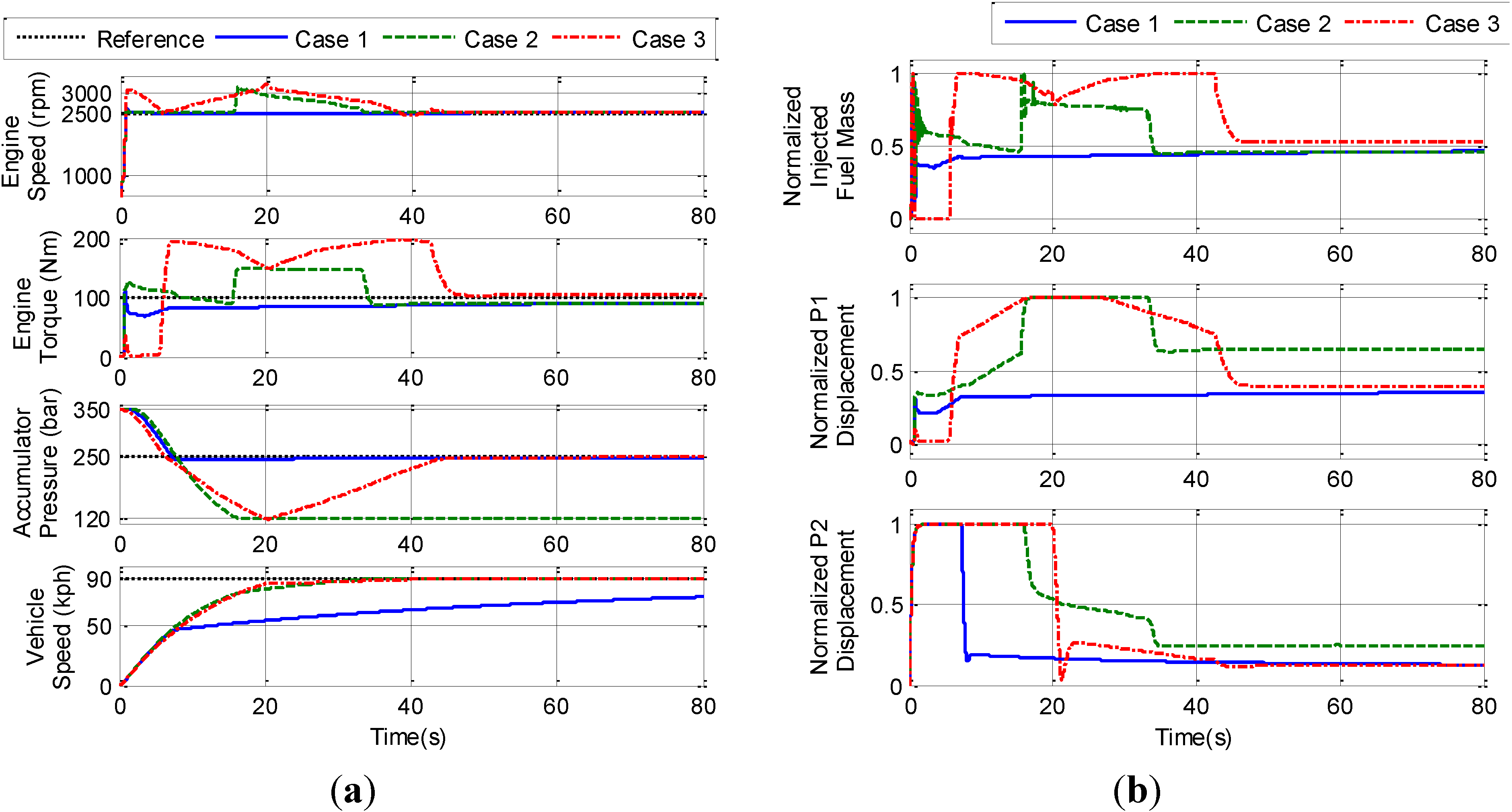
The behavior of the system under various weight factors is presented in Figure 9. In Case 1, engine speed reaches its reference value after just a short time. Engine torque approaches its reference value with some steady-state error. Accumulator pressure also reaches its reference value after 8 s. However, vehicle velocity cannot reach its reference value during the simulation time. In Case 2, the weight factor on the vehicle velocity is increased. The penalty on accumulator pressure is released. Vehicle velocity approaches to its reference value after 20 s. At 20 s, pressure in accumulator reaches its minimum threshold. Up to that point, the engine generated more power to fulfil the power demand. Hence, by handling this constraint, the MPC-based control system prevents the depletion of pressure in the accumulator. In Case 3, the four outputs are controlled to ensure that they approach their reference values. The results indicate that selecting suitable weight factors enables the MPC-based control system to designate various outputs in accordance with their reference values.
Focusing on regulating vehicle velocity and controlling engine, the output weight factors used in Case 2 were selected for simulations. With this approach, the controller regulates the vehicle velocity in accordance to desired driving cycles and controls the engine to operate at desired operating points.
Figure 9. Effect of weight factors on system performance: (a) Outputs; and (b) Inputs.
Energies 07 07017 g009
To evaluate the effectiveness of the proposed control system, two typical driving cycles, the Japan 1015 and the HWFET, were selected as reference trajectories. The Japan 1015 is used in Japan for emissions and fuel economy testing for light duty vehicles. This driving test presents typical stop-and-go patterns found in urban driving condition, which is an attractive application for HHVs. The HWFET, a chassis dynamometer-driving schedule developed by the US Environmental Protection Agency, is used to determine the fuel economy of light duty vehicles under highway condition.
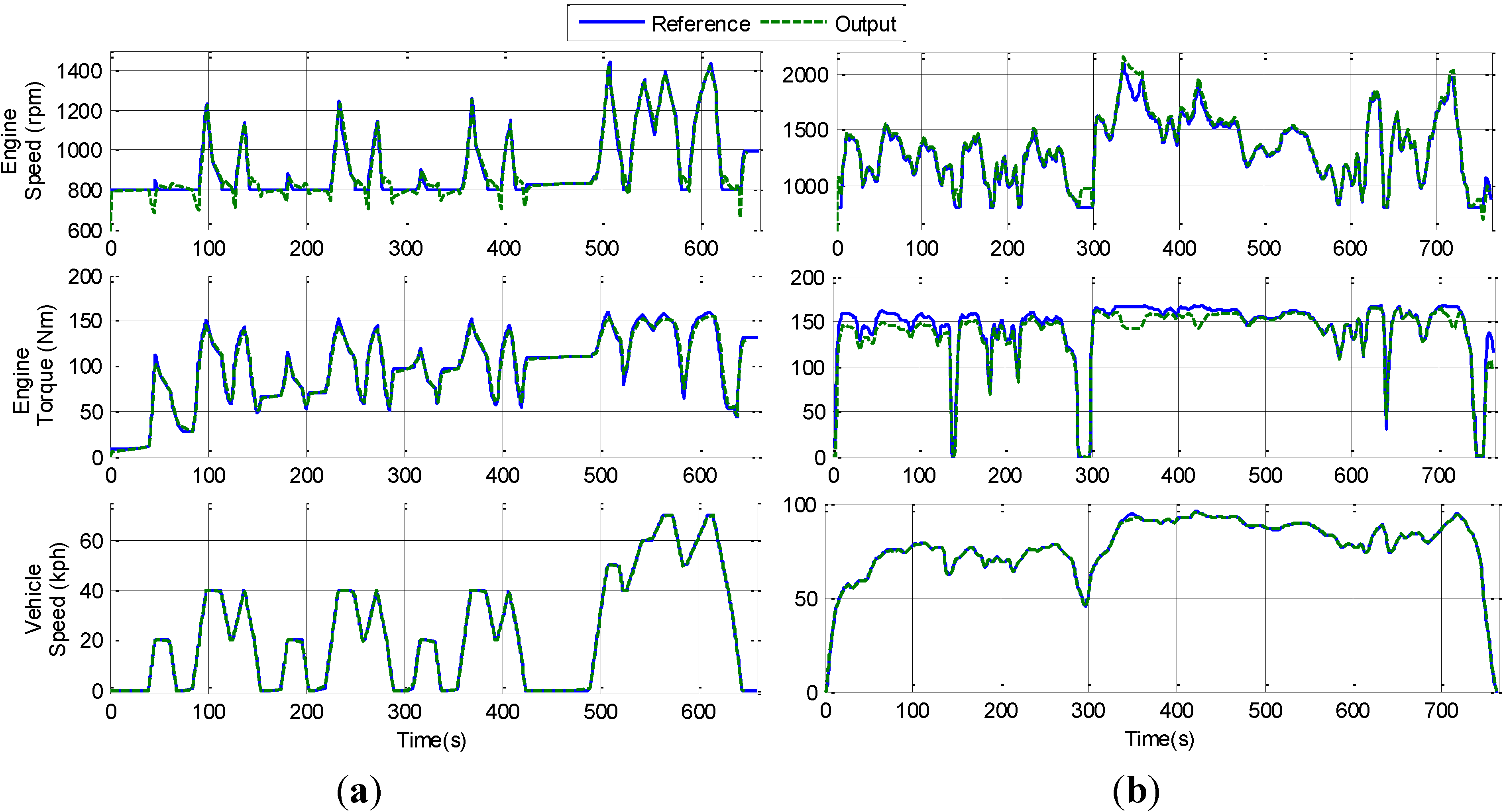
The behavior of the SHHV with the proposed control system are shown in Figure 10. The simulation results indicate that vehicle velicoty as wel as engine torque, engine speed, and accumulator pressure approach their reference values. As shown in the figures, the constraints on system inputs and outputs are internally handled by the controller without the need for any saturated component. Since the priority of tracking vehicle velocity is higher than tracking other outputs, a certain degree of tracking errors for engine speed, engine torque, and accumulator pressure is considered acceptable.
Figure 10. System behaviors: (a) Under Japan 1015; and (b) Under HWFET.
Energies 07 07017 g010
For comparison, a PID-based control system, developed in a previous work [
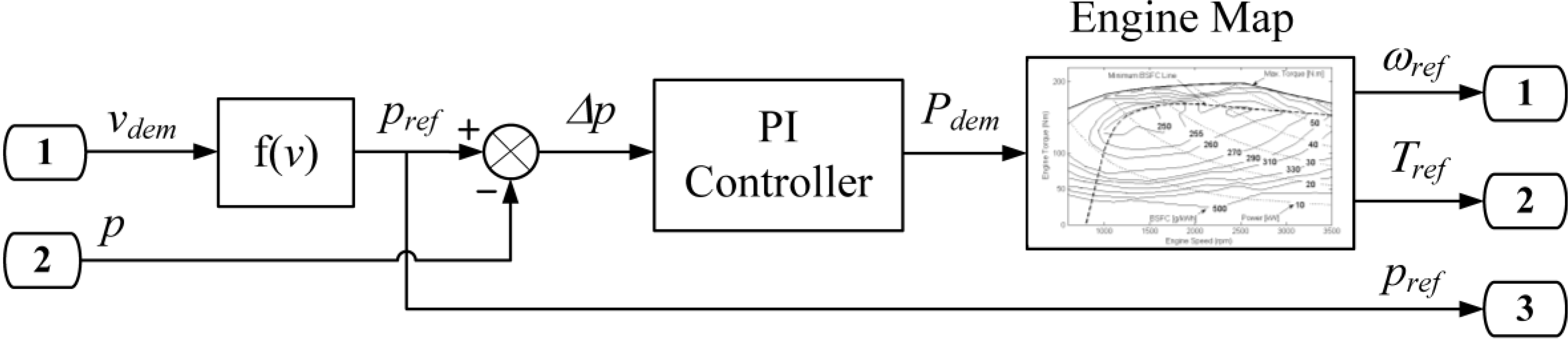
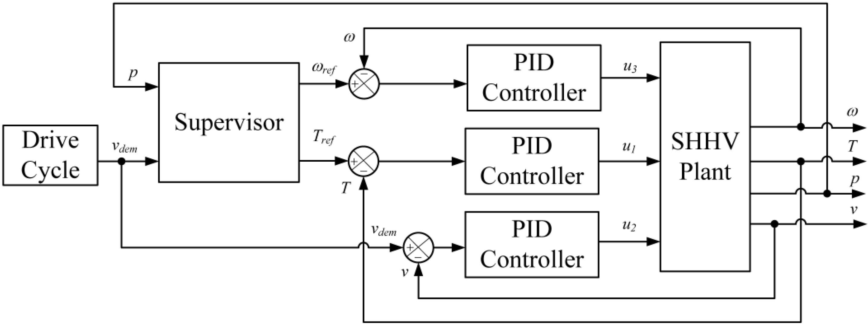
8], is used as a baseline. A diagram of this control scheme is shown in Figure 11. In this approach, three individual PID controllers are used to generate control signals. The first PID uses engine speed error as the input to calculate the control signal for the injected fuel mass of the engine, u3. The second PID adjusts the displacement of the pump, u1, to achieve the desired engine output torque. The desired vehicle velocity is obtained by adjusting the displacement of the pump/motor, u2. The supervisor determines the reference values for engine speed and engine torque according to the demand vehicle velocity and current pressure in the accumulator.
In an SHHV, the pressure of the accumulator must be maintained within a working range. The minimum working pressure must exceed the pre-charged pressure in order to avoid depletion. In this work, the pre-charge pressure was 100 bar, the minimum working pressure was 120 bar, and the maximum working pressure was 350 bar.
Figure 11. Schematic of the PID-based control system.
Energies 07 07017 g011
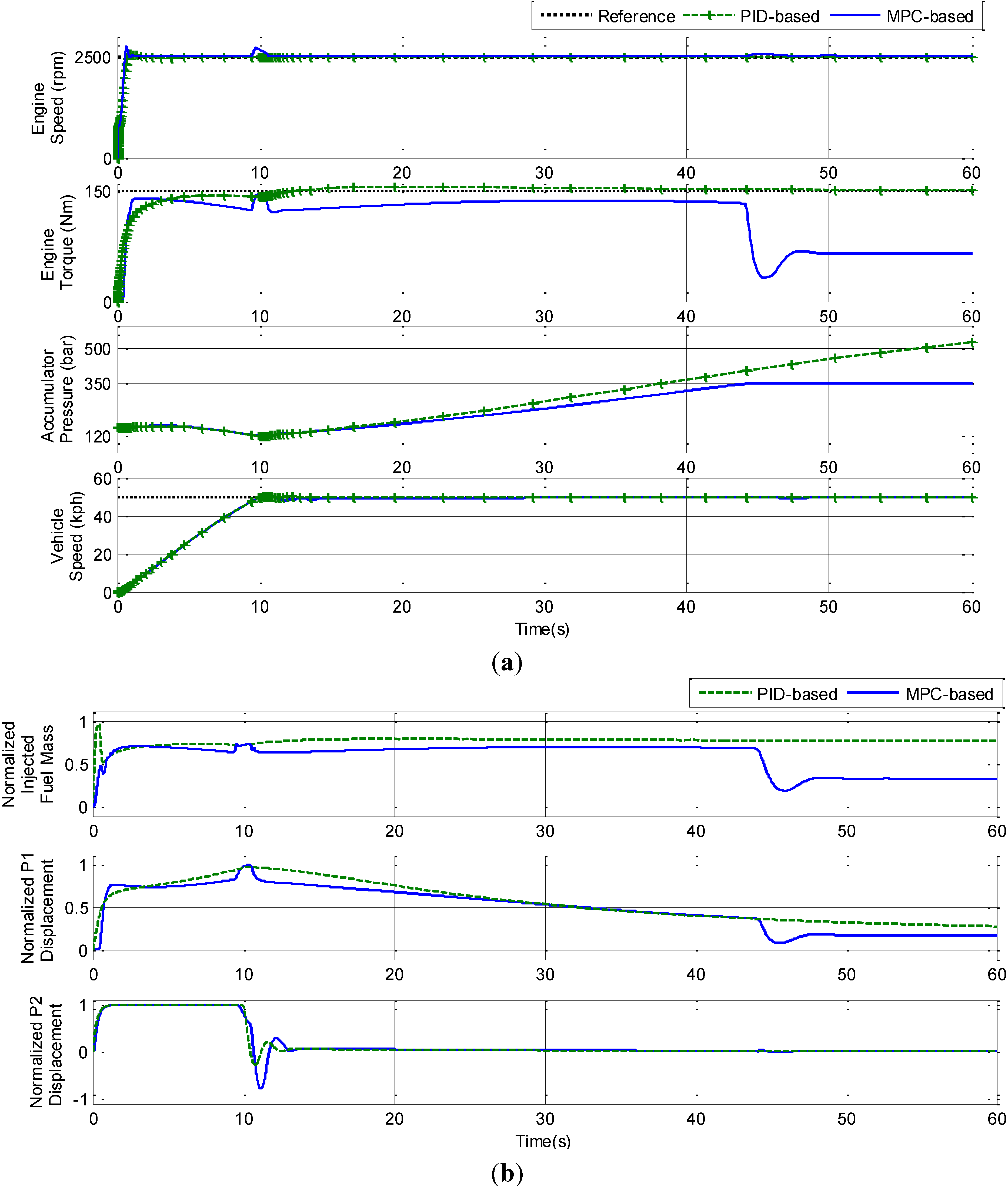
To evaluate the capability of constraint handling of the control systems, the SHHV was tested under two different sets of conditions, low and high target velocities. In both cases, the engine was demanded to operate at h the angular speed of 2500 rpm and the torque of 150 Nm. The target velocities were 50 and 90 kph, respectively. The behavior of the proposed and the baseline systems for these two cases are presented in Figure 12 and Figure 13, respectively.
Figure 12. The behaviors of the SHHV with a low speed demand: (a) Outputs; and (b) Inputs.
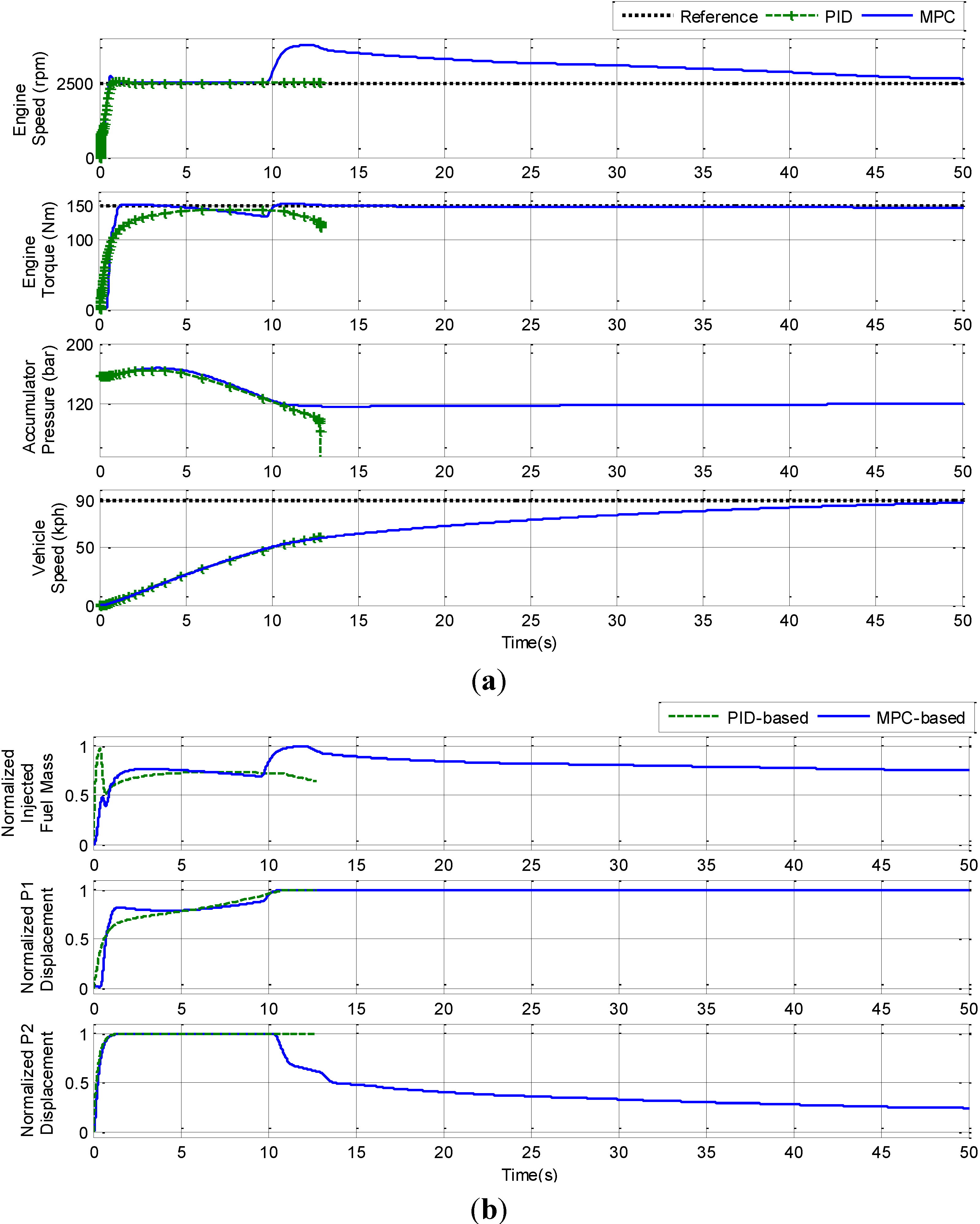
Energies 07 07017 g012
Figure 13. The behaviors of the SHHV with a high speed demand: (a) Outputs; and (b) Inputs.
Energies 07 07017 g013
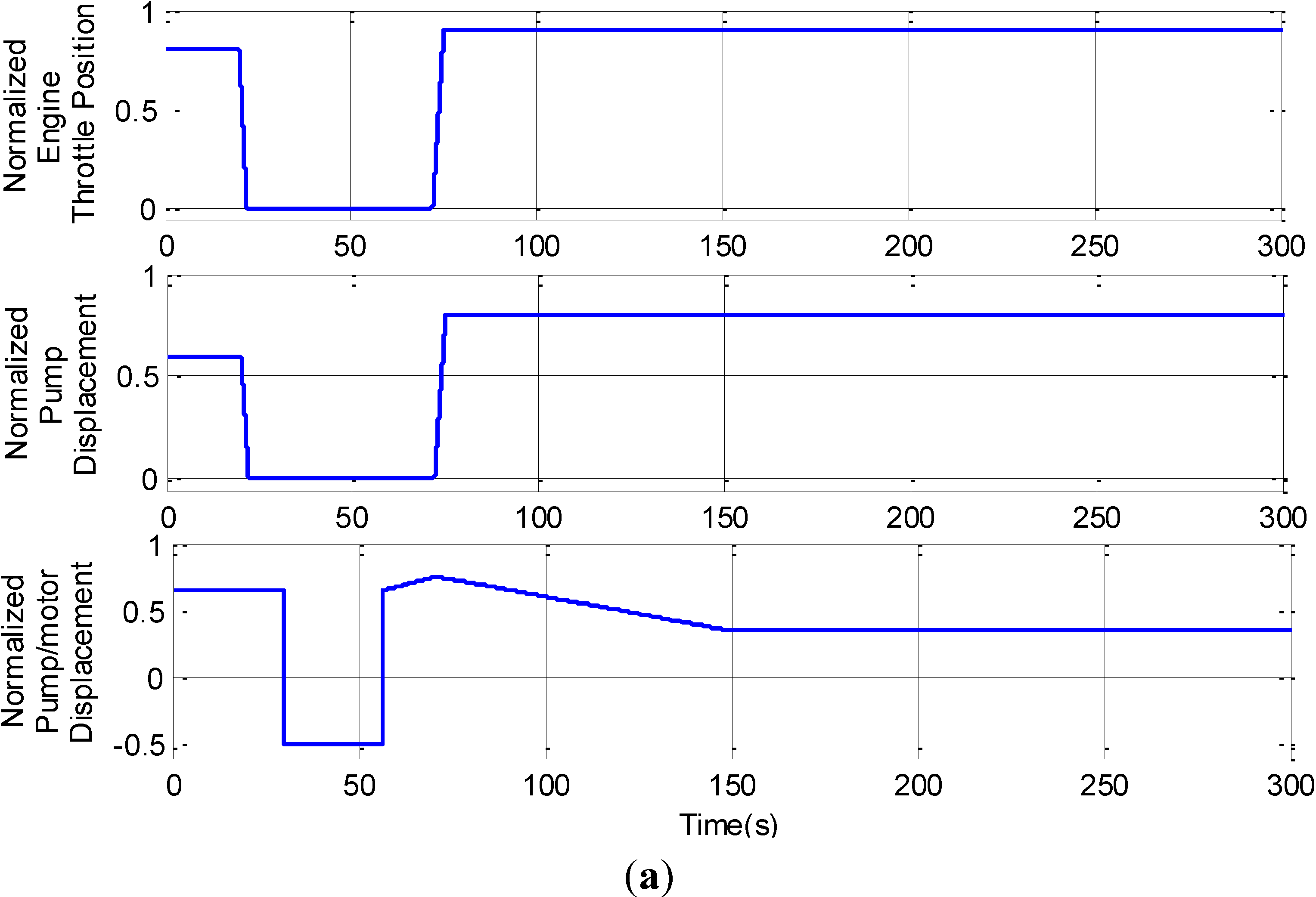
It can be seen that the inputs and outputs of the SHHV with PID-based and MPC-based control systems are initially quite similar. Difference only becomes apparent when pressure in the accumulator reaches its threshold. As can be seen in Figure 12, after the vehicle reaches the target velocity, the demand power becomes less than the engine power demand. The extra power is absorbed by the accumulator, which causes a gradual increase in pressure. In the PID-based control system, pressure in the accumulator continues increasing even after the maximum threshold has been reached (at 38.24 s). In contrast, the MPC-based control system reduces the engine injected fuel mass and pump displacement, such that the engine output power is reduced until it is equal to the demand. Thus, no additional power is converted for storage in the accumulator.
From Figure 13, it can be seen that after engine speed and engine torque have reached their reference values, engine power reaches a steady state. When the power demand of the vehicle exceeds the engine output power, the accumulator must make up the deficit. With the PID-based control system, accumulator pressure continues decreasing until the system failure at 12.76 s. Meanwhile, with the MPC-based control system, after 9.75 s, the injected fuel mass of the engine and the displacement of the pump were increased, such that the engine generated additional output power to satisfy the power demand. This strategy can help to avoid the system failure caused by the depletion of pressure in the accumulator.
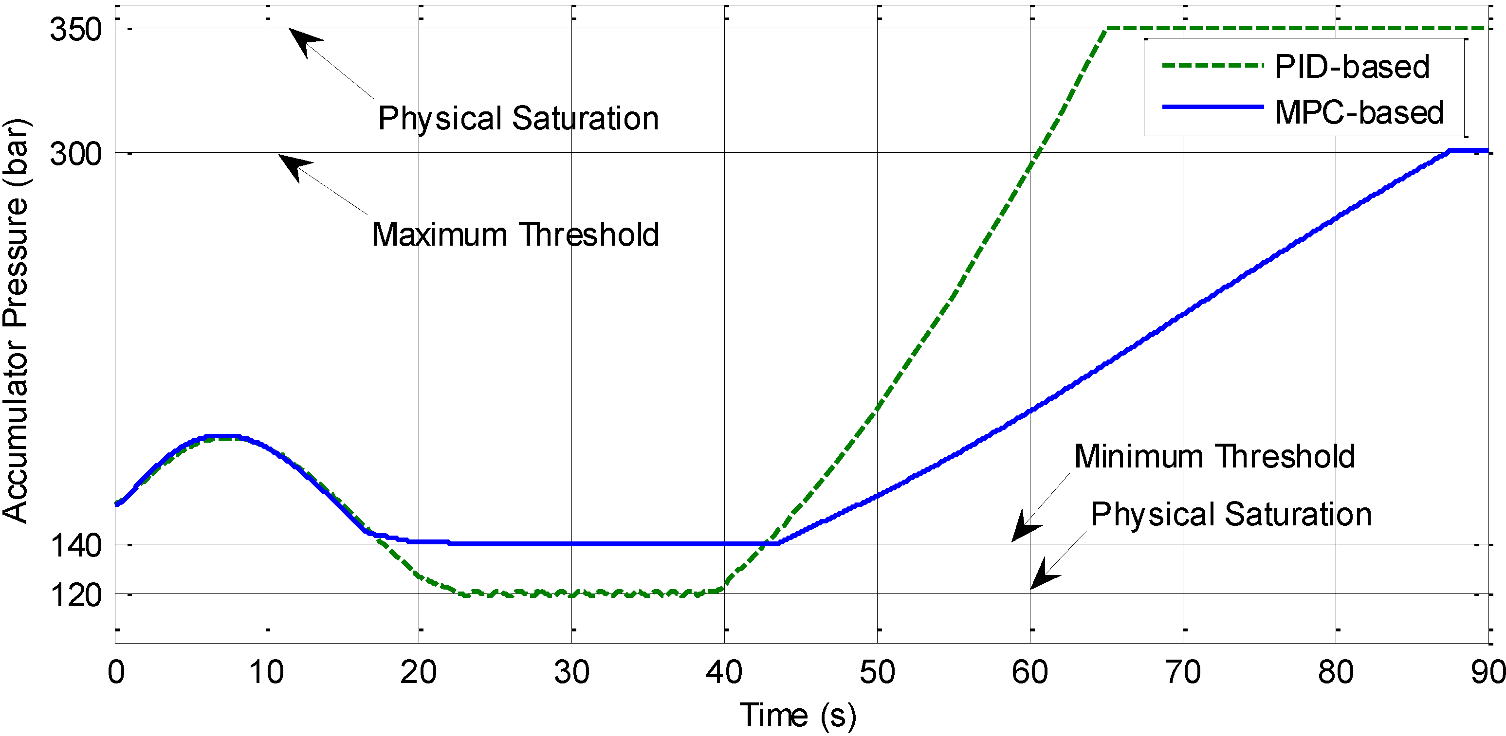
The behavior of the PID-based and MPC-based systems with physical saturation and state constraints is presented in Figure 14. In this case, the physical limitation of the accumulator pressure are 120 and 350 bar respectively. The minimum working pressure, 120 bar, is used to avoid the depletion of the accumulator while the high-threshold, 350 bar, is the maximum working condition of the accumulator. In addition, the pressure of the accumulator was maintained greater than 140 bar to ensure that the system can support the driving torque in any condition. The maximum threshold, 300 bar, is added to make sure that the accumulator reserves enough volume for recovering braking energy. The figure shown that in the PID-based system, pressure in the accumulator is maintained within the working range. However, using additional compensated valves will reduce efficiency of hydraulic system. In addition, the engine produced unnecessary power. When using the MPC-based control system, constraints on accumulator pressure are handled by the controller itself, thereby increasing the efficiency of the components.
Figure 14. Systems behaviors with physical saturations and state constraints.
Energies 07 07017 g014
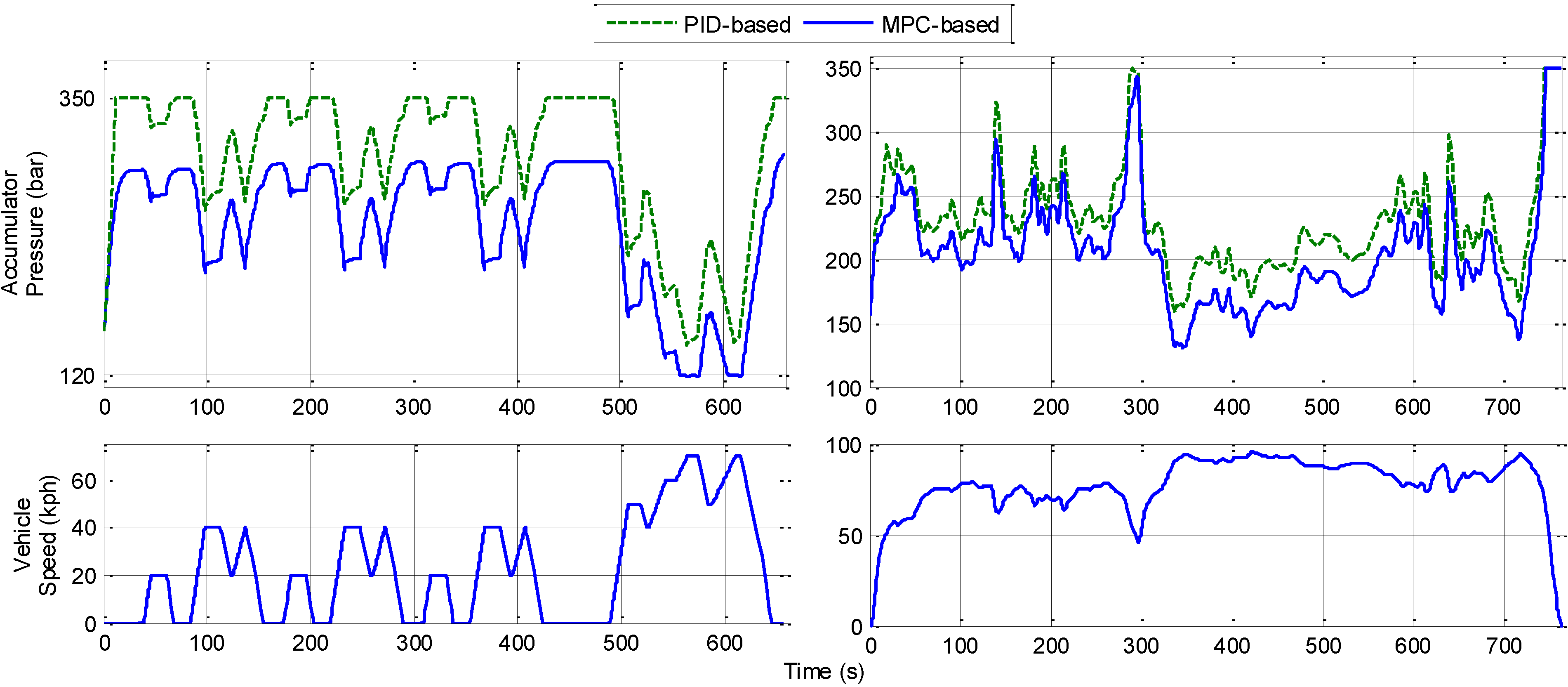
The performance of the SHHV with PID-based and MPC-based is presented in Figure 15. The results indicate that the accumulator pressure of the SHHV with the MPC-based control system is maintained at a lower value than that of the SHHV with the PID-based control system. In this way, unnecessary energy conversion from the engine to the accumulator is avoided, Thereby increasing the volume available for the storage of energy from regenerative braking.
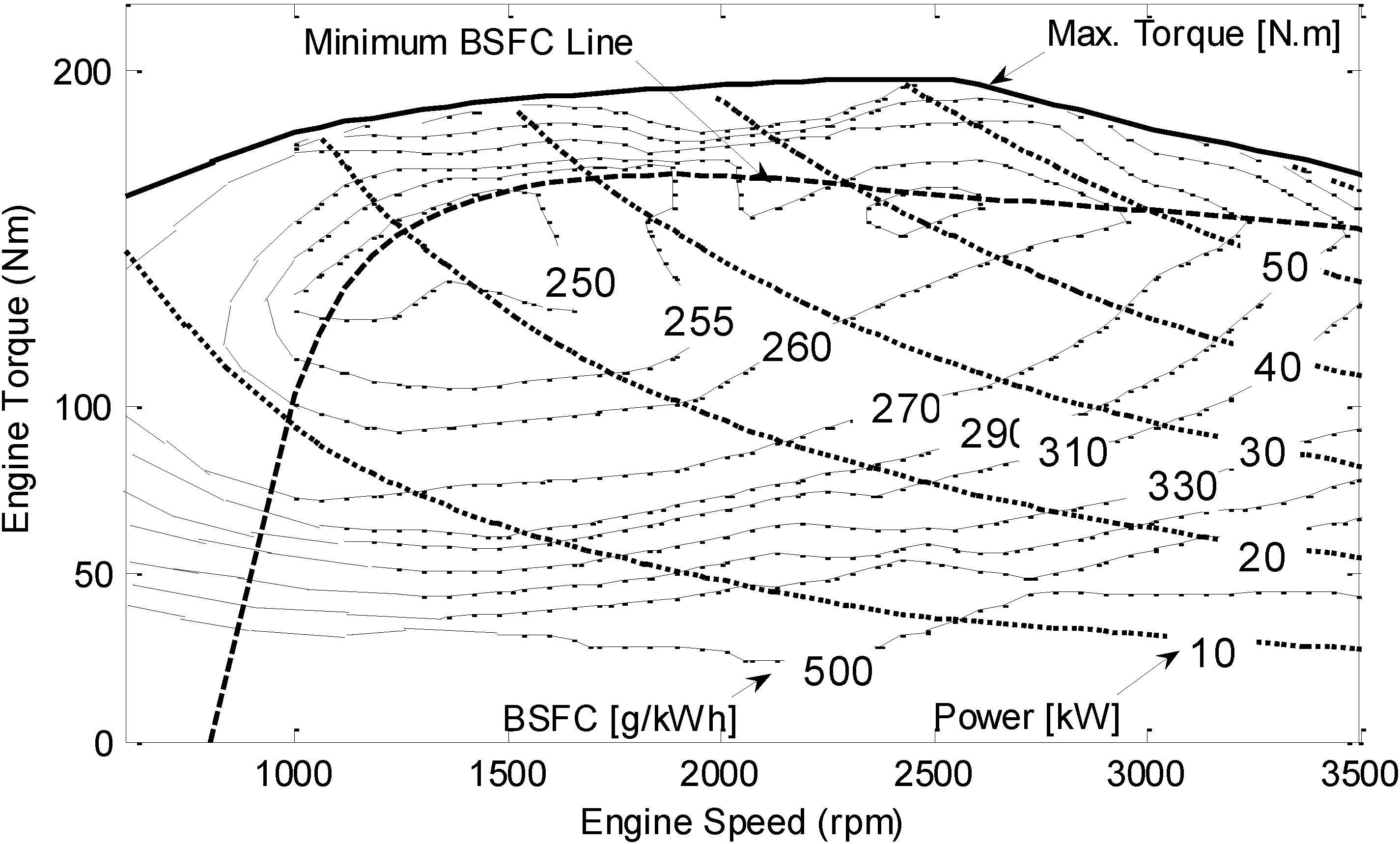
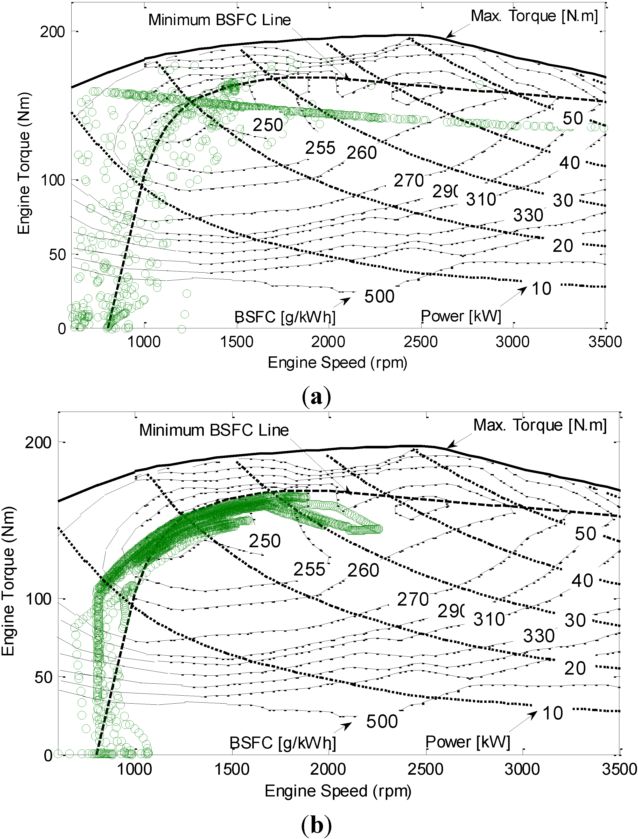
Figure 16 presents the distribution of the engine operating points under HWFET with the baseline and the proposed control schemes. It can be seen that the MPC-based control scheme keeps the engine operating in the sweet-spot region or along the minimum brake-specific-fuel-consumption (BSFC) line. In this way, the total fuel consumption of the engine is reduced and the fuel economy of the system is improved.
Figure 15. System behaviors under Japan 1015 driving cycle with MPC-based and PID-based control scheme.
Energies 07 07017 g015
Figure 16. Engine operating points visitation on the BSFC map under HWFET: (a) Using the PID-based control system; and (b) Using the MPC-based control system.
Energies 07 07017 g016
The fuel economy of the system using MPC-based and PID-based control system was evaluated under Japan 1015 and HWFET driving cycles. For each type of driving cycle, the simulation was conducted five times corresponding to the number of repetitions of the cycle from 1 to 5. The average fuel economy is listed in Table 4.
Table 4. Average fuel economy with different control schemes.
Control SchemeAverage Fuel Economy (km/L)
Japan 1015HWFET
PID-based11.3610.64
MPC-based15.3511.75
The results indicate that by capturing and reusing the braking energy, the SHHV achieves higher fuel economy when working under urban than under highway conditions. The ability of the MPC-based control scheme to manage the maximum and minimum thresholds of accumulator pressure ensures that the accumulator reserves sufficient volume for regenerative braking and prevents the system failure arising from the depletion of pressure in the accumulator. In contrast, preventing depletion of pressure in the accumulator under the PID-based control scheme requires that the minimum threshold for accumulator pressure be set high. This causes the engine to shift to a higher power region and limits the volume available for regenerative braking. The effect can be considerable when the system is working under a start-stop-and-go pattern such as Japan 1015. Thus, under Japan 1015, the MPC-based system improves fuel economy by 35% over that of the PID-based system. An improvement of only 10.43% is obtained under HWFET.

5. Conclusions

This study adopted an MPC-based framework for the design and evaluation of an energy management strategy for use in a SHHV. The effectiveness of the proposed system was evaluated and compared with the PID-based system under two typical driving cycles, representing urban and highway driving conditions, respectively. Managing input-output interaction and physical constraints allows reserving volume in the accumulator for regenerative braking energy and preventing unnecessary energy conversion. Thus, the MPC-based system obtains a noticeable improvement with respect to the PID-based system, particularly when the system is operating under urban driving conditions. Compared with the PID-based system, the MPC-based SHHV achieves a 35% improvement in fuel economy under Japan 1015 and a 10.43% improvement under HWFET.
The MPC framework presented in this work can be extended for other hybrid architectures. It also can be used to evaluate advanced energy management strategies. By predicting the future information of the system within a receding horizon, the MPC-based supervisory controller provides the capability to optimize the power split factor. Thus, optimal reference values will be achieved. Further studies will investigate the effect of replacing the PI controller in the supervisor by MPC.

Acknowledgments

The authors would like to thank the National Science Council of the Republic of China, Taiwan, for financially supporting this research under project number NSC 102-2221-E-212-004.

Author Contributions

All authors contributed to equal parts to the paper, whereby the first author was responsible for modeling the system, applying the MPC, and writing the initial manuscript. The corresponding author was mainly responsible for paper organizing, structuring, and revising the whole contribution. The third author participated in system simulation and manuscript formatting. All the authors read and approve the manuscript.

Conflicts of Interest

The authors declare no conflict of interest.

References

  1. Shan, M. Modeling and Control Strategy for Series Hydraulic Hybrid Vehicles. Ph.D. Thesis, University of Toledo, Toledo, OH, USA, 2009. [Google Scholar]
  2. Matheson, P.L.; Stecki, J.S. Modeling and simulation of a fuzzy logic controller for a hydraulic-hybrid powertrain for use in heavy commercial vehicles. SAE Tech. Pap. 2003, 2003. [Google Scholar] [CrossRef]
  3. Wu, B.; Lin, C.-C.; Filipi, Z.; Peng, H.; Assanis, D. Optimal power management for a hydraulic hybrid delivery truck. Int. J. Veh. Mech. Mobil. 2004, 42, 23–40. [Google Scholar]
  4. Filipi, Z.; Kim, Y.J. Hydraulic hybrid propulsion for heavy vehicles: Combining the simulation and engine-in-the-loop techniques to maximize the fuel economy and emission benefits. Oil Gas Sci. Technol. 2010, 65, 155–178. [Google Scholar] [CrossRef]
  5. Kim, Y.; Filipi, Z. Series hydraulic hybrid propulsion for a light truck-optimizing the thermostatic power management. SAE Tech. Pap. 2007, 2007. [Google Scholar] [CrossRef]
  6. Woon, M.; Nakra, S.; Ivanco, A.; Filipi, Z. Series hydraulic hybrid system for a passenger car: Design, integration and packaging study. SAE Tech. Pap. 2012, 2012. [Google Scholar] [CrossRef]
  7. Kim, Y.A. Integrated Modeling and Hardware-in-the-Loop Study for Systematic Evaluation of Hydraulic Hybrid Propulsion Options. Ph.D. Thesis, University of Michigan, Ann Arbor, MI, USA, 2008. [Google Scholar]
  8. Vu, T.V.; Chen, C.K.; Hung, C.W.; Chu, T.D. Integrated control system development for a series hydraulic hybrid Vehicle. In Proceedings of the 2nd International Conference on Intelligent Technologies and Engineering Systems (ICITES2013); Juang, J., Chen, C.-Y., Yang, C.-F., Eds.; Springer International Publishing: New York, NY, USA, 2014; pp. 1023–1030. [Google Scholar]
  9. Beck, R.; Richert, F.; Bollig, A.; Abel, D.; Saenger, S.; Neil, K.; Scholt, T.; Noreikat, K.E. Model predictive control of a parallel hybrid vehicle drivetrain. In Proceedings of the 44th IEEE Conference on Decision and Control and 2005 European Control Conference, Plaza de España Seville, Spain, 12–15 December 2005; pp. 2670–2675.
  10. Borhan, H.; Vahidi, A.; Phillips, A.M.; Kuang, M.L.; Kolmanovsky, I.V. Predictive energy management of a power-split hybrid electric vehicle. In Proceedings of the American Control Conference, St. Louis, MO, USA, 10–12 June 2009; pp. 3970–3976.
  11. Borhan, H.; Vahidi, A.; Phillips, A.M.; Kuang, M.L.; Kolmanovsky, I.V.; Cairano, S.D. MPC-based energy management of a power-split hybrid electric vehicle. IEEE Trans. Control Syst. Technol. 2011, 20, 593–603. [Google Scholar]
  12. Deppen, T.O.; Alleyne, A.G.; Stelson, K.A.; Meyer, J.J. A model predictive control approach for a parallel hydraulic hybrid powertrain. In Proceedings of the American Control Conference, San Francisco, CA, USA, 29 June–1 July 2011; pp. 2713–2718.
  13. Deppen, T.O.; Andrew, A.G.; Stelson, K.A.; Meyer, J.J. Optimal energy use in a light weight hydraulic hybrid passenger vehicle. J. Dyn. Syst. Meas. Control 2012, 134. [Google Scholar] [CrossRef]
  14. The Mathworks. Simscape Product Description. Available online: http://www.mathworks.com/help/physmod-simscape/gs/product-description.htm (accessed on 25 May 2014).
  15. Vu, T.V. Simulation and Design of Hydraulic Hybrid Vehicle. Master Thesis, Da-yeh University, Changhua, Taiwan, 2011. [Google Scholar]
  16. Pourmovahed, A.; Beachley, N.H.; Fronczak, F.J. Modeling of a hydraulic energy regeneration system—Part I. Analytical treatment. J. Dyn. Syst. Meas. Control 1992, 114, 155–159. [Google Scholar] [CrossRef]
  17. Tavares, F.; Johri, R.; Salvi, A.; Baseley, S. Hydraulic hybrid powertrain-in-the-loop integration for analyzing real-world fuel economy and emissions improvements. SAE Tech. Pap. 2011, 2011. [Google Scholar] [CrossRef] [Green Version]
  18. Maciejowski, J.M. A basic formulation of predictive control. In Predictive Control with Constraints; Prentice-Hall: Englewood Cliffs, NJ, USA, 2002; pp. 37–83. [Google Scholar]
  19. Goodwin, G.C.; Seron, M.; Dona, J.A. Constrained linear quadratic optimal control. In Constrained Control and Estimation—An Optimisation Approach; Springer: New York, NY, USA, 2005; pp. 103–124. [Google Scholar]

