The End of Cheap Oil: Economic, Social, and Political Change in the US and Former Soviet Union

Abstract

I use the quality and quantity of energy flows to interpret economic, social, and political changes in the US and Former Soviet Union. The economic successes of both the former Soviet Union (FSU) and the US reflect an abundant supply of high quality energy. This abundance ended in the 1970s in the US and the 1980s in the Former Soviet Union. In the US, the end of cheap oil caused labor productivity to stagnate, which stopped on-going growth in wages and family incomes. To preserve the American Dream, which holds that each generation will be better off than the one that preceded it, women entered the workforce, income was transferred from saving to consumption, the US economy changed from a net creditor to a net debtor, and debt held by families and the Federal government increased. Despite efforts to hide the income effects, the end of cheap oil also is responsible for increasing income inequality. In the FSU, the end of abundant energy supplies meant that allocating the energy surplus among the domestic economy, subsidized exports to Eastern Europe, and hard currency sales to the West became a zero sum game. This contributed to the collapse of the Council for Mutual Economic Assistance (CMEA) alliance and the FSU. If the US is able to extricate itself from personal and governmental debt, solving the social and political concerns about inequality is the next formidable challenge posed by the end of cheap oil.

1. Introduction

The Cold War can be viewed as the planet’s largest experiment. The methods section would be summarized as follows; divide the world’s population and their natural resources in half, operate market and centrally planned economies (CPE’s) in near isolation, let the experiment run for nearly a century, and compare results. The results section would highlight the collapse of the Soviet Union and CPE’s and the triumph of the US, Western Europe, and market economies. The standard discussion section would highlight the inherent superiority of market economies.

Here, I offer a different interpretation, one that highlights the importance of energy. The economic successes of both the former Soviet Union (FSU) and the US reflect the importance of energy and their failures are attributed to the end of cheap oil (Cheap oil does not refer to the purchase price. As explained below, it refers to abundant supplies (increasing rates of production) than can be extracted using small amounts of energy, capital, and labor relative to the quantity of oil extracted (high energy return on investment (EROI))). As long as high quality supplies of energy were abundant, both CPE’s and market economies provided their populations with a growing standard of living. Despite fundamental differences between the two economic systems, both succeeded by subsidizing human labor with ever-increasing quantities of fossil fuels, especially oil. This strategy was undermined by the end of “cheap oil”, which occurred during the early 1970s in the US and the late 1970s–early 1980s in the FSU. These dates often are associated with fundamental changes in both societies; the end of the US post-war economic expansion, the collapse of the Communist bloc, and the break-up of the former Soviet Union.

However, these highly visible economic and social changes rarely are linked to the energy. The Soviet Union credited central planning for its fifty-year transformation from a relatively backward agrarian society to a military and industrial power that was the first to launch a person into space and that “would bury (edit capitalism) [1]”. Similarly, popular rhetoric in the US credited its economic success to “free-market principles” and an emphasis on personal freedom. The collapse of the FSU often is attributed to economic inefficiency, economic stagnation, and bad policy choices, e.g., [2,3]. Conversely, the end of the US post-war expansion in the early 1970s is blamed on a host of technical and social factors, e.g., [4].

Here I argue that declining supply of oil triggered these political, social, and economic changes. Before proceeding, an important caveat. Social and economic changes in the FSU and the US were not determined by the quantity and quality of energy. Rather, changes in the quantity and quality of energy acted as a trigger. In both the US and the FSU, the declining quantity and quality of oil caused economic stagnation—but many economic, social, and political responses were possible. In the US, one response was a single-minded focus on cutting taxes. However, other responses were possible. In the Soviet Union, changes in the availability of energy made the allocation of oil a zero sum game; nonetheless the allocation chosen by the FSU was one of many possible solutions.

To offer an alternative explanation for economic, social, and political changes in the US and FSU, I describe the relation among energy supplies, economic production, and social relations in five sections. In the second section, I summarize theoretical arguments and empirical results that describe the importance of energy to economic activity. In the third section, I describe changes in the availability of energy (oil) to both the US and the FSU. The fourth section describes how changes in the supply of oil triggered economic, political, and social changes that hitherto, were not linked to energy. The final section concludes with a cautionary interpretation regarding the triumph of market economies and their flexibility in the face of rising inequality.

2. The Role of Energy in Economic Activity

Most microeconomic textbooks feature a simple but flawed model for economic activity [5]. This model shows exchange between households and firms. Firms produce goods and services, which are purchased by households. Households purchase those goods with income that they earn by selling factors of production such as capital and labor, to firms. Firms purchase these factors of production with the money that they earn by selling goods and services to households. According to this view, goods and services and the factors of production cycle endlessly between firms and households.

To those familiar with physics or engineering, this cycle is reminiscent of a perpetual motion machine. Although the laws of thermodynamics have long discredited the notion of a perpetual motion machine, those laws also undermine the basic economic model. From a thermodynamic perspective, economic activity can be interpreted as an increase in the organizational state of matter. Economic production extracts raw materials and organizes them in a way that suits human needs. For example, the timber industry harvests trees and sells them to industries that convert wood fibers to paper. Similarly, the electronics industry purchases metals and other raw materials and converts them into televisions, computers, iPods, etc.

Creating this economic order requires work. And work is possible only by using energy. Energy is required to chop down trees, separate the fibers, and compress them into paper. Energy is required to dig ores from the ground, separate useful metals from slag, and fashion the metals into useful products. From a thermodynamic perspective, energy is the sine qua non of economic activity.

The second law also dictates that the energy needed to power economic activity must come from the environment (i.e., energy cannot be recycled). As such, energy inputs influence the rate of economic activity. High rates of energy inputs allow an economy to produce significant quantities of goods or services. Conversely, low rates of energy input limit production to relatively small quantities. This general relation is consistent with empirical comparisons across nations. Countries that produce large quantities of goods and services consume large amounts of energy while nations that produce smaller amounts of goods and services consume smaller amounts of energy, e.g., [6,7].

This same relation holds over time. Within a single nation, there is a strong relation between the amount of energy consumed and the quantity of goods and services produced, e.g., [8]. Consistent with this notion, real GDP generated by the US economy increased 3.5 fold between 1929 and 1967 while energy use increased 2.5 fold [8]. A similar correlation prevailed in the FSU. Here, real GNP increased 7 fold between 1925 and 1965 while total energy use increased 35 fold [9]. In both market economies and CPE’s, economic production grew in conjunction with energy use.

The relation between energy use and the ability to produce goods and services is rooted in labor productivity, which measures the value of goods and services that a worker produces per unit of time. Highly productive workers produce more goods and services per time unit because their efforts are subsidized by large quantities of inanimate energy. For example, a carpenter with a nail gun can drive many more nails per hour than a carpenter with a simple hammer. Much of the technical progress of the last century consists of capital devices that increase the amount of fossil fuel that a worker can direct towards the production of goods or services. Consistent with these effects, labor productivity is positively related to energy use per worker hour over time in individual nations and across nations at any point in time [8,10,11].

Understanding the effect of energy use on labor productivity is critical because it is responsible for the increased material standard of living that is associated with the industrial revolution. In a market economy, a worker’s wage is equal to his or her productivity, as measured by value marginal product. Workers whose efforts are heavily subsidized by energy tend to be more productive, have higher wages, and enjoy a higher material standard of living. Under these conditions, increases in energy supply and/or energy price reductions that encourage energy consumption generally increase labor productivity, total economic activity, and income while constrictions in energy supply and/or higher energy prices slow increases in labor productivity, dampen economic growth, and cause income to stagnate. This “energy law” applies to both sides of the iron curtain and is the basis for economic success and failure in both the US and the FSU [12].

The link between economic activity and energy use can be weakened if the efficiency of using energy to produce economic output can be increased. In the short-run this is difficult because once capital is installed, its efficiency cannot be increased significantly. Returning to the example of the nail gun, the amount of electricity required to drive a nail by a given nail gun cannot be reduced significantly.

But the energy efficiency of capital equipment can be increased over time when old energy inefficient capital is replaced by newer, more efficient capital. Changes in macroeconomic energy efficiency sometimes are approximated by the amount of energy consumed to produce a unit GDP over time. This ratio increased at an annual rate of more than 4 percent in the FSU between 1925 and 1965 (declining efficiency), but declined at an annual rate of 0.7 percent (increasing efficiency) in the US [9].

The rapid rise in the energy/GDP ratio in the FSU probably is caused in part by declining energy efficiency. Energy prices in the FSU were significantly lower than world levels and so there was little incentive to develop new energy-efficient capital and/or replace old inefficient capital. Conversely, the declining energy/GDP ratio in the US probably overstates efficiency gains. Although the quantity energy supplied by different fuel types can be measured in heat units (e.g., BTUs), not all heat units are created equally. A heat unit of primary electricity can be used to do more economically useful work than a heat unit of oil or natural gas, which can do more economically useful work than a heat unit of coal (these differences are one reason why a heat unit of electricity has a higher price than a heat unit of oil and natural gas, which has a higher price than coal [13]. Indeed, when corrections are made for the types of fuels used and the types of goods and services produced, there is relatively little change in the quantity of energy used to produce a real currency unit of GDP in the US and other industrial nations [14,15]. As such, efficiency gains probably had relatively little effect on the large changes in energy supply that are described in the next section.

3. Energy Supply

The quantity of energy available to a society is measured by the energy surplus—the amount of energy that remains after the energy costs of recovering energy from the environment are subtracted. This relationship is represented as follows:

Energy Surplus = Energy obtained from environment − Energy used to obtain it

(1)

Surplus energy represents the quantity of energy that is available to do the work that people find useful—heat homes, run automobiles, power factories, etc. People do not want energy for energy’s sake. Think of an economy that extracts large amounts of energy, but uses all of that energy to extract next year’s energy supply. This economy consumes large quantities of energy, but none is “left over” to produce the goods and services that people want. Because of its small energy surplus, this economy generates a low material standard of living.

The ability of an energy resource to supply an energy surplus can be measured by energy return on investment (EROI), which is given by Equation (2):

$$EROI = \frac{Energy Obtained from Environment}{Energy Used to Obtain Energy}$$

(2)

According to Equation (2), fuels with a large EROI can supply large quantities of surplus energy to an economy. This surplus shrinks as EROI declines. Indeed, EROI sets a lower bound for useful energy resources. Using energy to recover a fuel deposit with an EROI of 1.0 or below does not contribute to an economy’s energy surplus, and so such deposits cannot be considered a viable source of energy, regardless of the quantity extracted.

Focusing on EROI and the energy surplus, as opposed to energy prices and the gross quantity of energy obtained from the environment is critical because both the US and Soviet economy contained distortions that could hide changes in the quality of energy supply. In the FSU, artificially low energy prices cause monetary measures to understate the importance of energy. In the US, the size of the energy surplus was distorted by tiered prices for crude oil and natural gas. In the 1970s, natural gas from “old” and “new” wells had a different price. This difference allowed firms to earn a profit by using a larger quantity of inexpensive “old” gas to produce a smaller quantity of higher priced “new” natural gas [16]. Despite this economic profit, these efforts reduced the surplus natural gas that was available to the US economy.

3.1. Changes in the Quantity of Oil Supply

The pattern of oil production over time is described by two types of models; economic, e.g., [17] and engineering, e.g., [18]. Hotelling’s [17] model tells a compelling story of resource extraction in a market economy. Owners of nonrenewable resources such as oil, produce oil over time in a way that maximizes its net present value. To do so, the model assumes that the owner knows how large his/her field is, the size of the total oil resource, and path over which demand and prices will evolve over time. Although consistent with the basic tenets of decision-making in a market economy, the model has little ability to explain the historical pattern of production or to forecast future rates of production [19]. As such, is called an intellectual cul-de-sac [20].

Conversely, economic principles are not represented explicitly in Hubbert’s model [18]. This model assumes that cumulative oil discoveries and production trace a logistic curve over time. Early in the cycle, cumulative production rises slowly because demand for oil is low and the ability to find/produce it is limited by technology. As technical capabilities to produce and consume oil grow, so too does cumulative production. Beyond some inflection point, the negative effects of resource depletion overtake the positive effects of increasing technical know-how, and this slows cumulative production. Eventually, cumulative production approaches an asymptote, which defines the ultimate recoverable supply of oil. This model defines a bell-shaped curve for annual rates of production.

Despite differences in the economic, social, political, and technical environments for oil extraction in the US and the FSU, Hubbert’s model captures the general pattern of production on both sides of the iron curtain. History validated the general outline of Hubbert’s model when oil production in the lower 48 states peaked in 1970, which matched the forecast made by Hubbert in 1956. Furthermore, oil production declined nearly continuously after 1970, despite large increases in oil prices, drilling rates, and extraction technologies. These changes did, however, slow the rate of decline relative to those predicted by Hubbert [21,22,23,24].

Similarly, the Hubbert curve captures the general pattern of production in the FSU. In 1977, the CIA [25] used Hubbert’s model to forecast that Soviet oil production would peak in the 1980s. Although some greeted this forecast skepticism, e.g., [26,27], production in the FSU peaked a second time in 1988, after an initial peak in 1983. Production declined much faster than predicted by the Hubbert model because the Soviet economy collapsed. However, unlike in the US, production rebounded back towards the previous peak when new technologies and market signals rationalized production in Russia and the newly independent states [28].

3.2. Changes in the Quality of Oil Supply

Changes in oil production described by the Hubbert model are exacerbated by changes in the quality of oil supply. As described previously, the peak in oil production is caused in part by the cost-increasing effects of depletion overtaking the cost reducing effects of technical gains. This implies that the EROI for oil will start to decline at about the same time that production peaks. The reduction in EROI, which was caused by increasing amounts of energy required to extract energy, reduced the energy surplus in a way that amplified the reduction in the quantity of oil obtained from the environment (Equation (1)). The synergistic effects of declining production and a shrinking EROI reduced the energy surplus, which defines the end of “cheap oil” in both the US and the FSU.

In both the US and the FSU, the EROI for domestic oil production declined at about the same time as production peaked. The EROI for US hydrocarbon production (crude oil, natural gas, and natural gas liquids) peaked in 1972 at 23:1 and dropped to 10:1 in 1983 [29]. Although this drop seems small, the ratio (Equation (2)) implies that this reduction in quality reduced the energy surplus from US hydrocarbons by about 6 percent. This reduction, coupled with the 10 percent decline in production during the same period, caused a significant drop in the energy surplus from domestic oil production.

The data needed to calculate the EROI for oil production in the FSU are not available, nonetheless, I approximate changes in EROI based on annual rates of production and capital investment in the oil industry. Capital investment is used to proxy the cost of obtaining oil because oil production is very capital intensive. Data for real capital investment in oil production (real 1984 Rubles) are available starting in 1960 [30]. Between 1960 and 1978, rates of investment and production followed each other, such that oil production in 1978 was 3.9 times greater than production in 1960 while annual investment in the oil industry in 1978 was 4 times greater than it was in 1960. These parallel rates of increase imply a relatively stable EROI.

After 1978, growth rates for investment and production diverged sharply. Between 1978 and 1988 (the last year for which data are available), annual investment in oil production increased 2.7 fold, but the annual rate of production increased by about 10 percent. The rapid increase in capital investment with little increase in production implies that increasing amounts of capital were used to extract each unit of oil. This increasing capital cost caused a significant decline in the EROI for oil production in the FSU. This conclusion is reinforced by an economic analysis, which indicates that the marginal cost of extracting oil and natural gas in the FSU increased from 6 rubles in 1970 to 24 rubles in 1978, but then rose to 92 rubles in 1985 [31]. Coupled with the decline in production, the increasing cost of production implies that the FSU suffered a sharp decline in its domestic oil surplus starting in the late 1970s.

Both the US and FSU could have offset declines in domestic oil production by importing oil. The US pursued this strategy; oil imports increased from 6 million barrels per day in 1973 (34 percent of consumption) to 8.6 million barrels per day in 1977 (47 percent of consumption) [32]. However, the increase in imports overstates their contribution to the US energy surplus. The US (and other nations) “pay” for oil by exporting non-oil goods, which require energy to produce. Because the price of oil rose significantly in the 1970s, the quantities of goods and services (and the energy used to produce them) that were exchanged for a barrel of oil also increased. In addition, the increased quantity of goods and services exchanged for oil reduced the EROI for imported oil. The EROI for US oil imports declined from more than 30:1 before 1973 to less than 10:1 in the early 1980s [33]. The decline in EROI meant that increasing imports did not offset completely the decline in the energy surplus that was caused by producing less domestic oil from lower quality fields. For reasons that will be described below, importing oil was not a viable option for the FSU.

4. Energy Related Economic, Social, and Political Changes the US and Former Soviet Union

The peak in domestic oil production and the associated decline in EROI coincide with important economic, social, and political changes in the US and FSU. In the US, the declining supply and quality of oil coincided with the end of the postwar economic expansion (To test whether there are meaningful changes in economic or social indicators and whether these changes coincide with the changes in the energy surplus, I fit a simple equation to the time series Y (Y_t = α + βYear_t + μt) and test whether the constant (α) and/or trend (β) changes in a statistically meaningful fashion using a test statistic developed by Bai and Perron [34]. This test statistic is generated by estimating the following equation ${\mu }_t=\varphi +{\gamma }_{1}Yea{r}_t+{\gamma }_{2}D{T}_{t}Yea{r}_t+{\epsilon }_t$ in which $DT=1(Yea{r}_t>Yea{r}_{Break})\times (Yea{r}_t-Yea{r}_{Break})$ and Year_Break is the year of the break. I allow for up to five breaks, each of which has a minimum size of 10 observations. The number of breaks is chosen using the test statistic and the timing of these breaks is described below. I recognize that these results are not definitive given that the time series probably are not trend stationary). In the FSU, the declining supply and quality of oil coincided with the end the end of the “communist bloc” and the Soviet Union itself [35]. In this section, I describe how these changes can be interpreted as possible responses to a shrinking energy surplus.

4.1. Social and Economic Responses to Shrinking Oil Surpluses in the US

In a market economy, a shrinking oil surplus is perceived through the lens of higher oil prices. In 1973–1974, the real price of oil increased about 40 percent (EIA). Prices rose another 190 percent between 1979–1981, such that the real price of oil in 1981 was $61 per barrel (2005$), compared to $13 (2005$) in 1970. Prices shrank back to 1974–1975 levels in 1986, but even the Asian financial crisis did not drop prices to the level that prevailed during the post war expansion. In addition, after 2000, prices rose steadily from $30 (2005$) to $85 ($2005) in 2012.

Before describing the impacts of the 1973–1974 price increase, a short aside on how this price increase is related to the declining quantity and quality of US oil production. Prior to 1973, the US acted as the marginal supplier of oil [36]. The Texas Railroad Commission (and other state commissions) maintained price stability by opening and shutting spare capacity to balance supply and demand [37]. Following this strategy, the Texas Railroad Commission allowed only 30 percent of capacity to operate in 1963. After that trough, Texas lost its spare capacity such that fields operated at 100 percent of capacity in 1973 [37]. At this point, the US lost its ability to offset OPEC production decisions. As such, OPEC became the marginal supplier of oil in 1973 and thereby gained the ability to influence price [38,39]. The potential for this loss of spare capacity to affect OPEC’s ability to influence oil prices was described six months before the October 1973 oil shock in the April 1973 issue of Foreign Affairs [40].

Higher oil (energy) (Oil prices drive changes in the price of other fuels [41,42] undermined the basic strategy that powered US economic growth during the previous sixty years. As energy prices rose relative to capital and labor, it no longer made economic sense to subsidize labor with increasing quantities of energy. Consistent with this change, US energy consumption increased 0.8 percent per year between 1975 and 2012, as opposed to 3 percent per year between 1950 and 1975 [32].

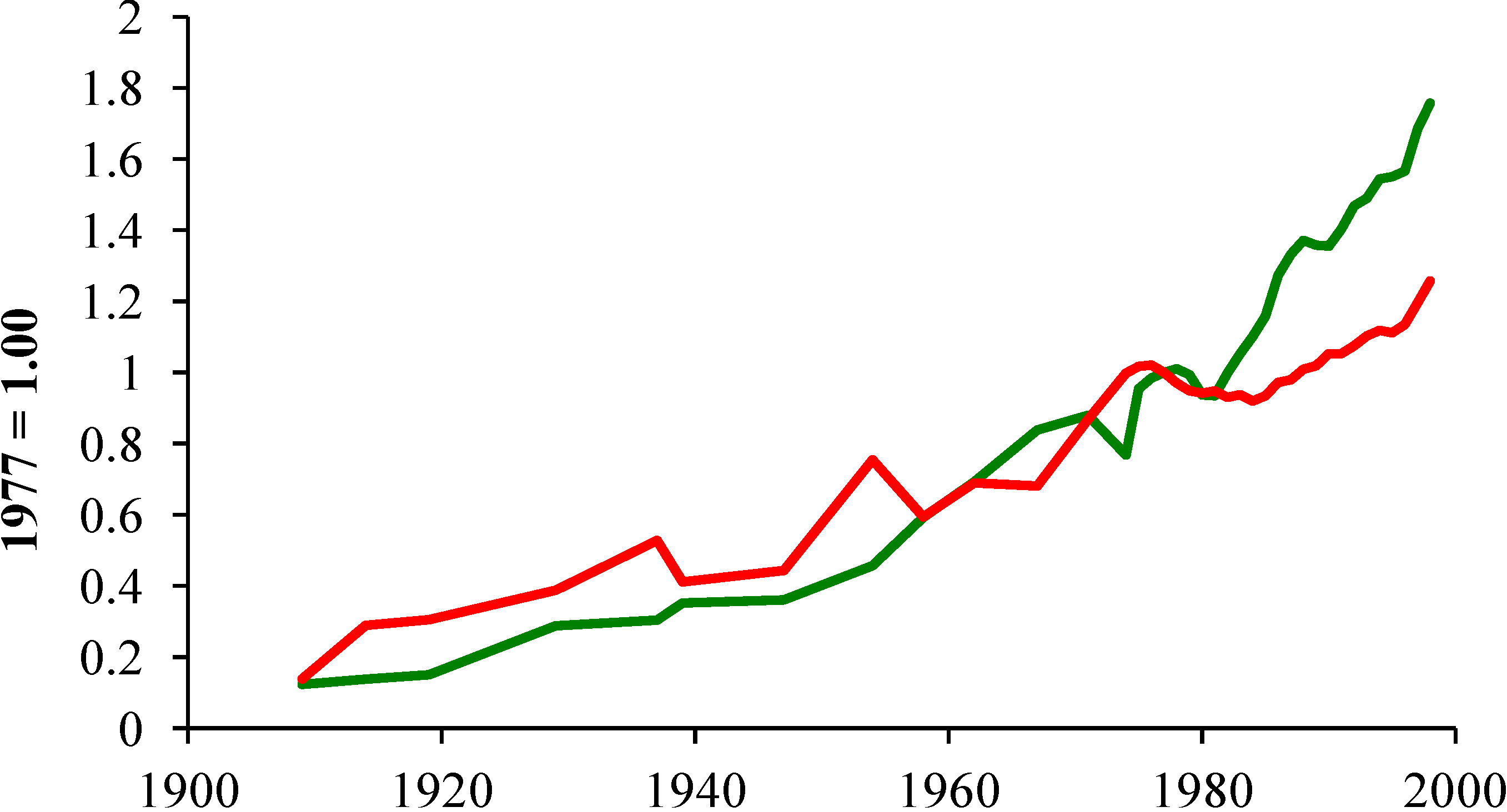
The slow-down in energy consumption relative to population growth ended the steady growth in the quantity of energy used per worker hour in the US (Figure 1). Without more nail guns or more powerful tractors, carpenters no longer drove more nails per hour and farmers did not expand the amount of land he/she cultivated. This stagnation slowed technical change, labor productivity, and economic growth.

The emphasis on energy supply separates cause and effect. Labor productivity stagnated for more than a decade starting in the early 1970s because the end of cheap oil undermined the economic logic of subsidizing labor with increasing quantities of energy. Put simply, the marginal return to technical innovation declined in large part because the cost of implementing those innovations increased.

Although the slowing the growth of energy consumption per worker was not discussed widely, its effects on the US economy were highly visible. As the amount of energy used to subsidize workers stopped growing, the marginal product of labor stopped growing.

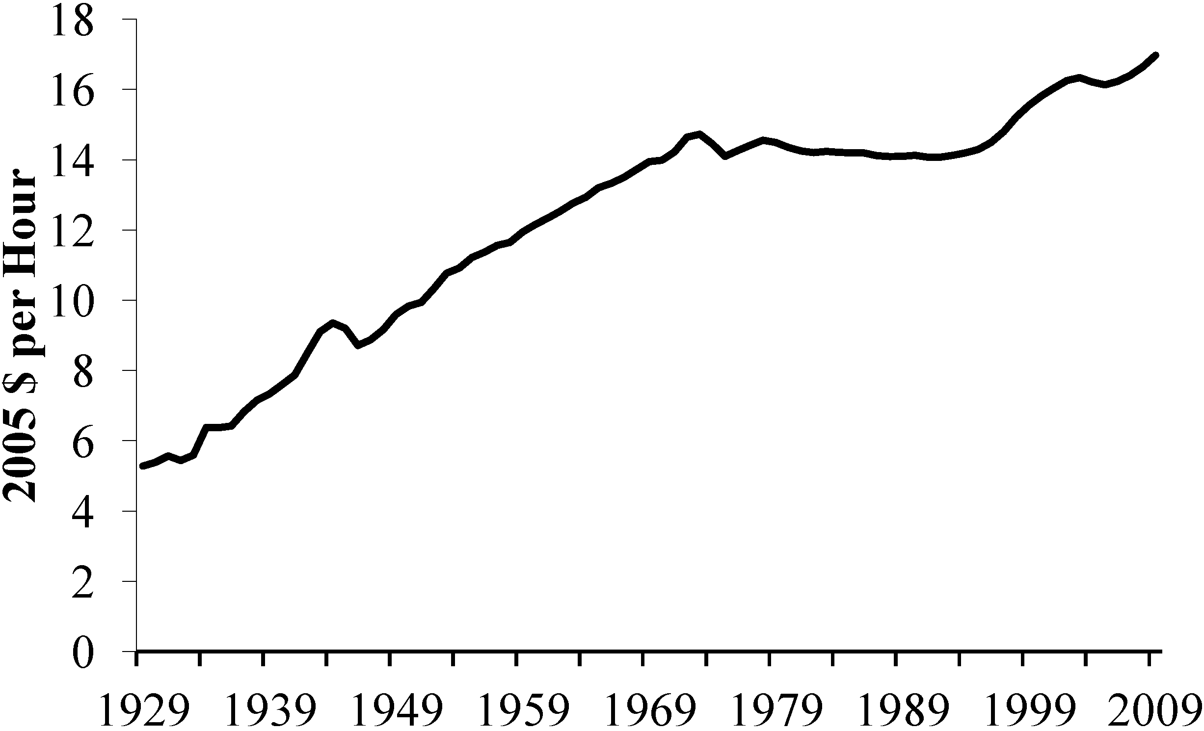
Consistent with this thermodynamic axiom, wages stopped growing in the early 1970s (Figure 2). Statistical tests identify two breaks in the time series for real wages, 1973 and 1996 (if a single break is imposed on the data, the break occurs in 1979, the time of the second oil shock). Consistent with the first break, real wages (2005$) in manufacturing grew in the forty-plus years from 1929 ($5.28) through the 1973 ($17.72). However, after 1973, real wages were constant for nearly 25 years. Wages did not rise beyond the 1973 level until 1997, which coincides with the second break identified by statistical tests.

Figure 1. The relationship between energy use per worker hour (red line) in the manufacturing sector and labor productivity (green line) in the manufacturing sector for the entire period for which data are available. Data for energy use, production worker hours, and value added use are from Annual Survey of Manufacturers (various years). Data for value added are deflated by PPI. Both time series are divided by their respective values in 1977 to derive an index with a base value of 1.0 in 1977.

Figure 1. The relationship between energy use per worker hour (red line) in the manufacturing sector and labor productivity (green line) in the manufacturing sector for the entire period for which data are available. Data for energy use, production worker hours, and value added use are from Annual Survey of Manufacturers (various years). Data for value added are deflated by PPI. Both time series are divided by their respective values in 1977 to derive an index with a base value of 1.0 in 1977.

Figure 2. Real wages ($2005) in the US manufacturing sector. Data from the Bureau of Labor Statistics [43].

Figure 2. Real wages ($2005) in the US manufacturing sector. Data from the Bureau of Labor Statistics [43].

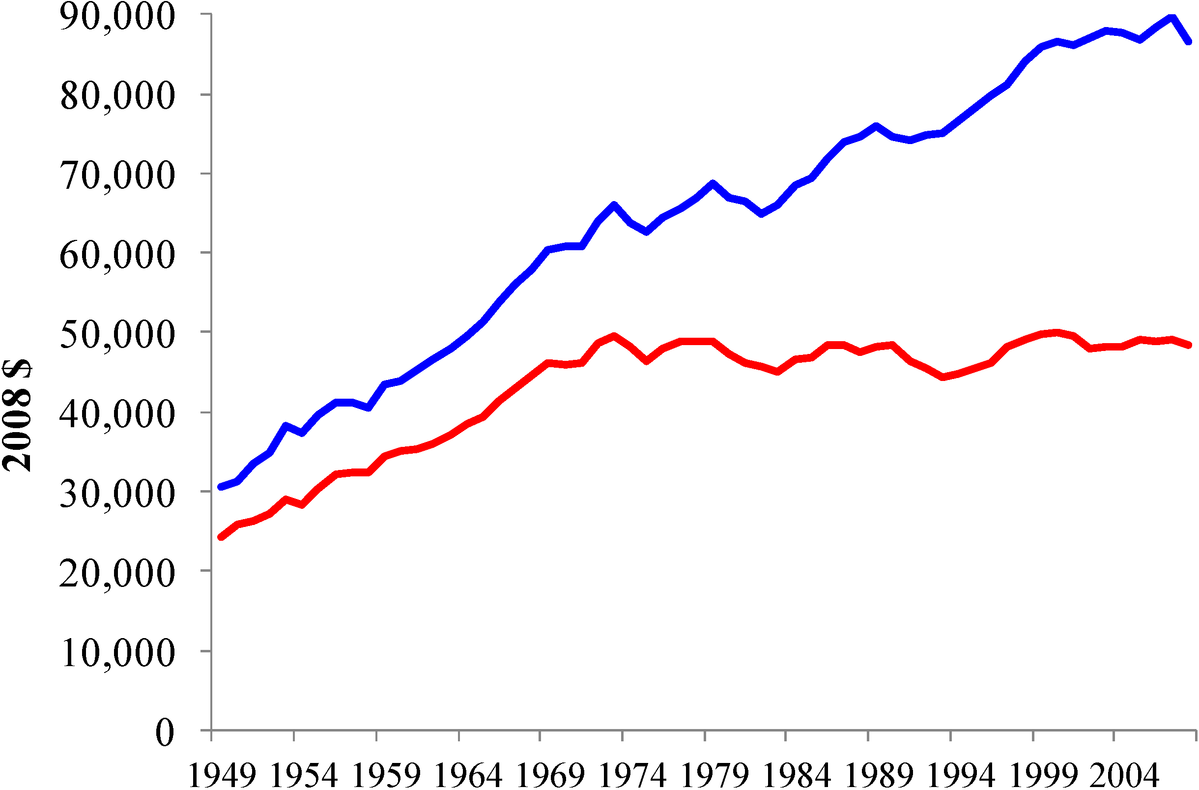
The sudden end in wage increases was mirrored by real family income (Figure 3). Statistical tests identify two breaks, 1971 and 1996. Real income for families with a single male income rose steadily from $24,200 ($2008) in 1949 to $46,200 ($2008) in 1971. After 1971, real family income with a single male breadwinner did not rise significantly. In 2008, income for the “traditional” American family was $48,500, only slightly more than the $46,200 in 1971.

The lack of income growth violated an important component of the American Dream; each generation will be financially “better off” that the one that precedes it [44]. Although average income for males in the baby boom generation did not rise, this stagnation did not stop families from trying to increase their standard of living. These efforts triggered a series of economic, social, and political changes that are described below.

Figure 3. Median real family income for married couples in which wife is not in the paid labor force (red line) and wife is in the paid labor force (blue line). Data from the Bureau of Labor Statistics [43].

Figure 3. Median real family income for married couples in which wife is not in the paid labor force (red line) and wife is in the paid labor force (blue line). Data from the Bureau of Labor Statistics [43].

In an era of slow wage growth, one way to expand family income was to increase the number of workers per family—specifically have women work outside of the house. Consistent with this strategy, female participation rates increased from 43.3 percent in 1970 to 50.9 percent in 1979. This 7.6 percentage point increase was the largest decadal rise in the twentieth century. For comparison, the female participation rate rose 5.6 percentage points in the 1960s and 1980s.

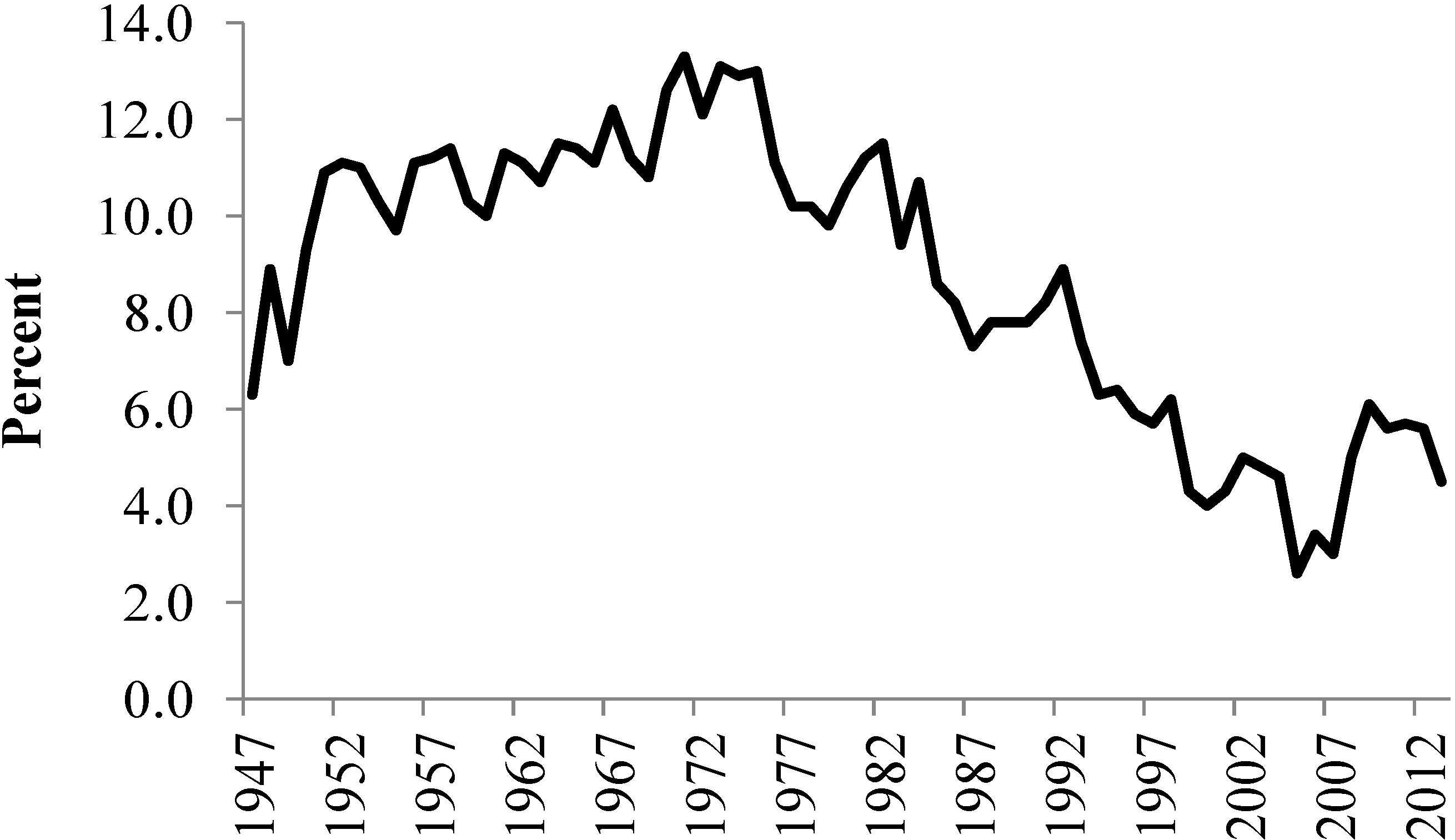
Because increasing female participation rates generated only small increases in family income (Figure 3), families pursued other strategies. One strategy supplemented consumption by reducing the savings rate. This time series of the US savings rate shows two breaks, 1975 and 1998. Between 1947 and 1975, the US savings rate grew (Figure 4). These savings were used to fund investments in new capital, which increased the productive capacity of the economy, and to pay for “big ticket items”, which were purchased by consumers. After 1975, the US savings rate declined.

Lowering the savings rate to supplement stagnant family incomes prompted changes elsewhere in the economy. By reducing the domestic savings rate, the US economy had to rely on to foreign sources of capital. This helped reverse the international investment position of the US economy. During the post war economic expansion, the US had a positive international investment position (a net creditor). This position was reversed in 1986, when the US became a net debtor nation (negative position). This position became increasingly negative thereafter.

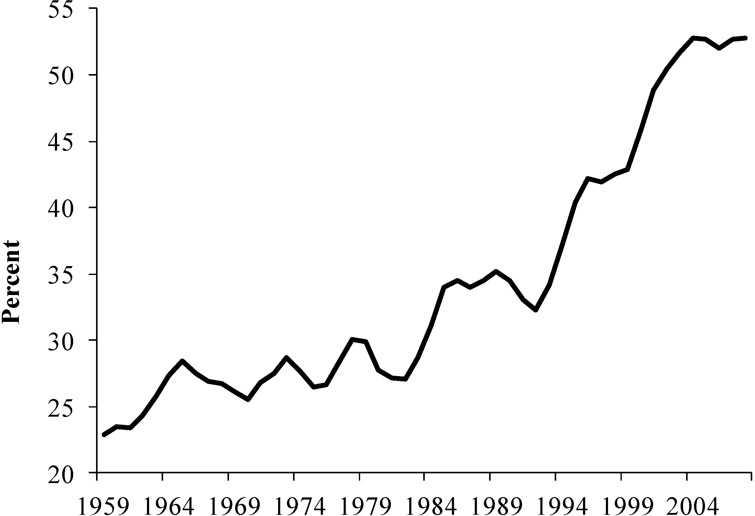
At the individual level, savings were no longer available to fund large purchases. To maintain/increase their standard of living, consumers continued to expand their purchases, but relied on credit. Consumers’ reliance on credit can be measured by the ratio of outstanding consumer credit (divided by the number of US families), divided by median family income. By this measure, outstanding consumer credit rose slowly but steadily between 1959 and 1993 (Figure 5). However, after 1993, statistical tests indicate a measureable acceleration such that outstanding consumer credit exceeded 50 percent of family income in 2002.

Figure 4. Personal saving as a percentage of disposable personal income, percent, annual, not seasonally adjusted. Data from US Federal Reserve Bank of St. Louis [45].

Figure 4. Personal saving as a percentage of disposable personal income, percent, annual, not seasonally adjusted. Data from US Federal Reserve Bank of St. Louis [45].

Figure 5. Outstanding consumer credit, divided by the number of families and average family income. Data from the Board of Governors of the Federal Reserve System [46].

Figure 5. Outstanding consumer credit, divided by the number of families and average family income. Data from the Board of Governors of the Federal Reserve System [46].

Assuming debt to maintain or expand living standards extended to the government through a single-minded focus on cutting taxes. Single minded because the Federal government cut taxes, which reduced government receipts, without cutting government outlays. Outlays were not cut because government purchases and services support economic wellbeing by simulating demand and by supporting individual incomes. In short, this strategy inflated economic well-being by allowing citizens to enjoy the benefits of government services without paying for them. Not surprisingly, this “something for nothing” strategy proved to be politically popular.

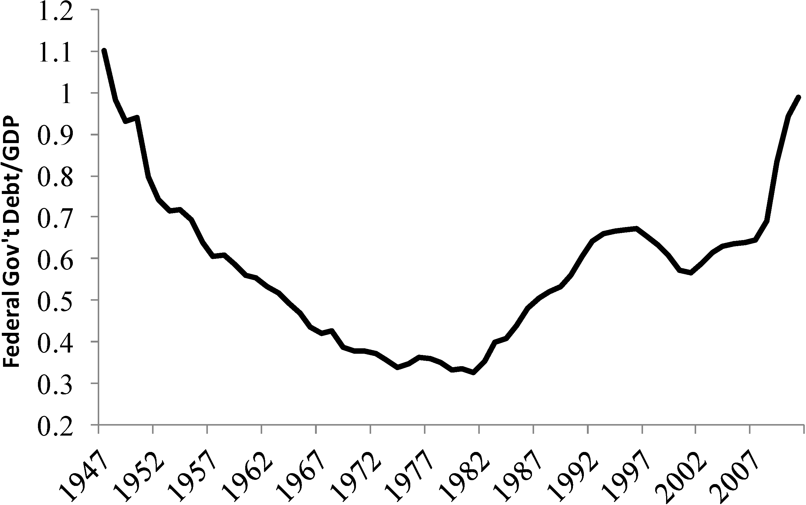
To reap the benefits of government services without paying for them, the electorate chose to add the costs of unfunded services to government debt. During the post war economic expansion, outlays by the federal government were a relatively constant fraction of GDP (15–20 percent). Despite occasional deficits that were associated with recessions (economic slow-downs reduce tax receipts), the US government paid off debts incurred during World War II. By doing so, the ratio of US Federal Government debt to GDP declined steadily from 120 percent in 1946 to 34 percent in 1971 (Figure 6). Statistical tests indicate identify a break in 1977, after which the ratio starts to rise, with a second break in 1996. By 2011, the ratio of US Federal Debt to GDP was 99 percent, which equaled its 1948 value.

Figure 6. US Federal government debt as a faction of current year GDP. A value of 1.0 indicates debt equals the current year’s nominal GDP. Nominal values of GDP and US Federal government debt are obtained from US Government Printing Office [47].

Figure 6. US Federal government debt as a faction of current year GDP. A value of 1.0 indicates debt equals the current year’s nominal GDP. Nominal values of GDP and US Federal government debt are obtained from US Government Printing Office [47].

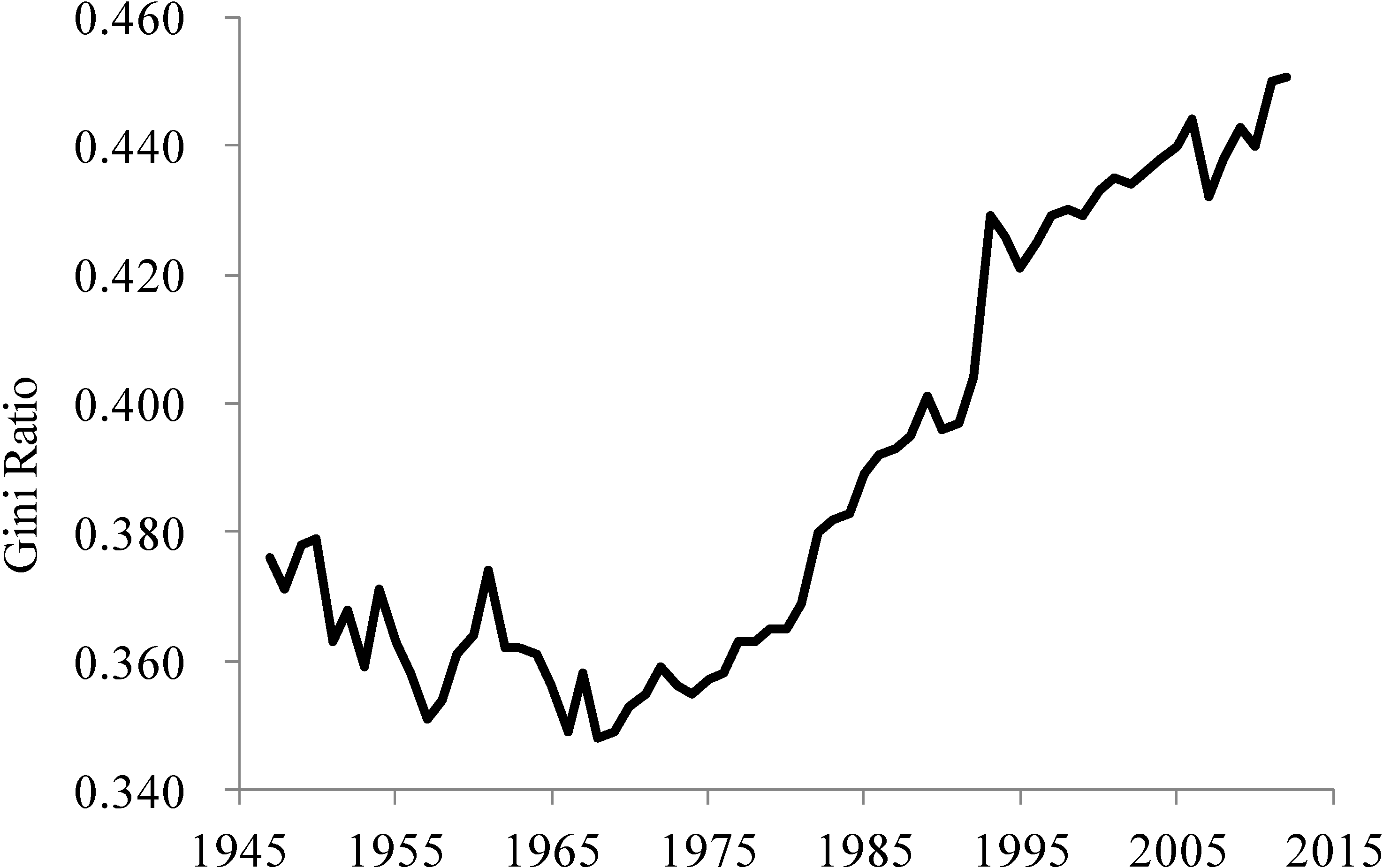
Despite efforts to hide the income effects, the end of cheap oil also is responsible for increasing income inequality. Cheap oil created the world’s first large middle class. This middle class was supported largely by manufacturing jobs, which subsidized workers with increasing amounts of energy and so supported high wages. These high wages and rising family incomes reduced income inequality between 1947 and 1972, as measured by Gini ratios (zero indicates all values are equal whereas a value of one indicate maximum inequality among values) for all US families (Figure 7).

Figure 7. Gini ratios for all US Families. Data from U.S. Census Bureau [48].

Figure 7. Gini ratios for all US Families. Data from U.S. Census Bureau [48].

Without abundant supplies of cheap oil, the US economy lost many of its manufacturing jobs. Without these jobs, a significant fraction of the displaced workers (and new entrants to the labor force) were forced into jobs that were not subsidized by large amounts of fossil fuels, such as retail. Without a large energy subsidy, these jobs pay lower wages, and the shift towards these “less energy subsidized sectors” reversed the US economy’s post-war movement towards greater equality. Statistical tests indicate that income inequality started to grow in 1972 and continued to rise through 2012 with a second jump in 1990.

4.2. Collapse of the Communist Bloc and the Former Soviet Union

Like the US, the FSU used the increasing quality and quantity of oil to support a growing standard of living for its inhabitants. However, unlike the US, the FSU used their expanding supply of oil for three purposes; to raise domestic living standards (to ensure domestic peace), to earn hard currency (to pay for imports from the West), and to expand sales to East European allies (to ensure cooperation). As long as the quantity and quality of its domestic oil production expanded, the FSU was able to satisfy these three economic and political objectives. However, the end of cheap oil in the FSU created a zero sum game in which the FSU had to choose among allocating its surplus to the domestic economy (to sustain domestic peace), to subsidized exports to Eastern Europe (to sustain cooperation), and to hard currency sales to the West (to import food and technology).

Many allocations among these three uses are possible; the FSU cut energy allocations to all three uses. Some of the decline in the energy surplus was allocated to the domestic economy, which undermined the strategy for domestic economic growth that succeeded during the previous half century. The productivity of both capital and labor inputs declined sharply between 1976 and 1980 relative to previous five year periods [49]. For example, annual growth in labor productivity declined from about 4 percent between 1961 and 1975 (3.9 percent in 1971–1975) to 0.6 in 1976–1981 and −0.5 percent in 1981–1982 [49]. Consistent with this slowdown, the growth rate for total industrial output slowed from about 6 percent between 1960–1975 (5.9% between 1971–1975) to less than 3 percent from 1976–1982 [49].

Perhaps the most obvious (and damaging) example of domestic energy shortages is illustrated by agricultural problems in the fall of 1989. Although both official policy and black markets provided considerable incentives, crops that were ready for harvest rotted in the fields. Reynolds [35] argues that this failure occurred because domestic shortages of gasoline and diesel prevented farmers from harvesting crops and prevented truckers from transporting them to market.

Some of the decline in the FSU energy surplus also was allocated to Council for Mutual Economic Assistance (CMEA) allies. During the Soviet post war economic expansion, many East Europe nations were largely dependent on imports to satisfy their oil demand, and most of these imports came from the Soviet Union. For example, Poland imported about 97 percent of the oil it consumed between 1970 and 1994 and over 90 percent of this oil originated in the FSU. As such, oil from the FSU was an important source of energy for Eastern Europe.

The Soviet Union used this dependence as both a carrot and a stick. To nurture dependence by their partners in the CMEA, the FSU sold oil to CMEA customers at below market prices [50]. In 1974, the FSU sold crude oil to its East European allies at $2.50 per barrel (the world price was about $10 per barrel). Such sales reduced Soviet revenues and discouraged improvements in energy efficiency. Conversely, CMEA allies were cut-off from inexpensive sources of oil if they rebelled (e.g., Hungary, 1956; Czechoslovakia, 1968).

As production stagnated and the world price of oil rose, each barrel sold to CMEA allies at below market prices cost the FSU increasing quantities of hard currency. To keep up with rising prices, the FSU set prices for the East European allies based on a three-year running average. In 1989, the FSU announced a 10 percent supply cut for 1990 and required CMEA nations to pay for oil in hard currency [50]. Higher prices and lower supplies caused economic difficulties for East European nations and reduced incentives for economic cooperation.

Finally, reductions in the oil surplus reduced the FSU’s ability to earn hard currency from oil exports. The reduction in hard currency reduced the economy’s ability to pay foreign debts and import food and technology. These changes reduced living standards both in the short run (fewer consumer goods) and the long-run (less technology based capital investments).

The political and economic uses of the energy surplus by the FSU (as opposed to the largely economic use by the US) and the collapse of the FSU (as opposed to economic and social changes within the US economic system) greatly complicates any link between the declining energy surplus and the collapse of the FSU. There is no simple cause and effect relation between a declining energy surplus and socioeconomic collapse in the FSU (as opposed to social and economic changes within the existing system in the US). There might have been no collapse if the Soviets had used a different allocation, if the economy had more efficient, if its administrators had been less corrupt, and/or had there been more (or less) economic reform under perestroika. Although these “what-ifs” prevent me from drawing a straight-line from the declining surplus to collapse, the timing and magnitude of this decline and the creation of a zero sum game is consistent with Reynolds’ [35] conclusion “Certainly, there were many factors that played a role in the fall of the Soviet Union. Nonetheless, the straw most capable of breaking the proverbial camel’s back was oil”.

5. Conclusions: The Triumph of Market Economies

About ten years later than the US, the former Soviet Union experienced the same decline in their energy surplus. However, unlike the US, where the end of cheap oil triggered a series of political, economic, and social changes that allowed the system to persist, the response to the end of cheap oil on the other side of the iron curtain triggered the end of the “communist bloc” and eventually the Soviet Union. Although oil was not more important to CPE’s, their social and political organization did not support the flexibility that allowed market economies to persist.

The success of the US and market economies lay in their ability to communicate changes in the availability of energy. Although not communicated perfectly, market economies were able to transmit information about the end of cheap oil more effectively than CPE’s. In the US and other market economies, that flexibility generated the economic, social, and political changes described above. The fundamental nature of these change are easily underappreciated from the vantage of 2014. Consider women’s integration into the workforce. Within the span of thirty years, popular TV shows went from the 1950s Honeymooners, in which Alice hides her efforts to earn money by babysitting [51], to shows such as Roseanne, in which the lead character, a working woman, is a normal aspect of life.

This is not to say that the US escaped the consequence of the end of cheap oil. Without taking a position on whether market economies require constant growth, the US economy and its consumers have not given up the notion that each generation will be materially “better off” than the one that precedes it. Without this recognition, the US economy postponed the day of reckoning by consuming savings and borrowing against future income. Now that the size of the economic pie has stopped growing (on a per family basis), social and political issues that focus on the size of the slices will become increasingly important. Solving the economic, social, and political concerns about inequality is the next formidable challenge posed by the end of cheap oil.