Modeling and Design Optimization of Variable-Speed Wind Turbine Systems

Abstract

As a result of the increase in energy demand and government subsidies, the usage of wind turbine system (WTS) has increased dramatically. Due to the higher energy production of a variable-speed WTS as compared to a fixed-speed WTS, the demand for this type of WTS has increased. In this study, a new method for the calculation of the power output of variable-speed WTSs is proposed. The proposed model is developed from the S-type curve used for population growth, and is only a function of the rated power and rated (nominal) wind speed. It has the advantage of enabling the user to calculate power output without using the rotor power coefficient. Additionally, by using the developed model, a mathematical method to calculate the value of rated wind speed in terms of turbine capacity factor and the scale parameter of the Weibull distribution for a given wind site is also proposed. Design optimization studies are performed by using the particle swarm optimization (PSO) and artificial bee colony (ABC) algorithms, which are applied into this type of problem for the first time. Different sites such as Northern and Mediterranean sites of Europe have been studied. Analyses for various parameters are also presented in order to evaluate the effect of rated wind speed on the design parameters and produced energy cost. Results show that proposed models are reliable and very useful for modeling and optimization of WTSs design by taking into account the wind potential of the region. Results also show that the PSO algorithm has better performance than the ABC algorithm for this type of problem.

1. Introduction

Wind power as a potentially available free energy resource has experienced a rapid growth in the world since the 1990s due to the limited quantity of fossil fuel resources. A wind turbine system (WTS) transforms kinetic energy into electrical energy and it primarily consists of an aeroturbine, which converts wind energy into mechanical energy, a gearbox that serves to increase the speed and decrease the torque, and a generator used to convert the mechanical energy into the electrical energy [1]. These systems have two types of operation: fixed-speed (constant) and variable-speed power generation. In the fixed-speed type of WTS, the generator is connected directly to the distribution grid through a transformer and the rotor speed is kept constant by using the stall principle or pitch control. Under fixed-speed operation, the tip-speed ratio changes with the variation of wind speed, which leads to the change of rotor power coefficient as well as the power output [2]. With the rapid development in the field of power electronics, variable-speed wind energy conversion systems have been designed and are commonly used for energy production. Under variable-speed operation, the rotor speed is controlled by a control unit to maximize power output and to decrease the torque of loads. In order to produce electrical energy at a maximum level, the most appropriate operation is to change the turbine speed with the wind speed yielding a continuously maintained tip-speed ratio to keep power coefficient at maximum. In the cases when the wind speed is lower than the rated speed, for maximum power point, the rotor speed must be adjusted and maintained. When the wind speed is higher than the nominal speed, the power output is decreased by controlling the pitch angle of the blades [2,3].

There has been several ways to reduce the capital and operation investments in wind energy conversion systems. One of them is to optimize the capture of energy from the wind utilizing effective control strategies [4–7]. The contributions of these studies include new control structures, even for the aeroturbine mechanical part [4,6,7] and the electrical components [5–7] that overcome some of the drawbacks of existing control methods. For the mechanical part control, the control design is generally based on a local linearized model of the WTS around its operating points [4]. Some nonlinear controllers were also proposed assuming that the wind turbine operates under steady state conditions [6,7]. For the generator, a doubly fed induction generator (DFIG) with a power converter is a common and efficient configuration to transfer the mechanical energy from the variable speed rotor to a constant frequency electrical grid [6]. The stator is directly connected to the grid while the rotor is fed through a variable frequency convertor. In order to produce electrical active power at constant voltage and frequency, the active power flow between the rotor circuit and the grid is controlled both in magnitude and direction by controlling the stator flux and rotor current of the asynchronous generator using standard nonlinear [5,6] and/or adaptive control techniques [7,8].

Another efficient way to reduce cost of a WTS is through optimal wind farm planning and predictive maintenance. The main objective of optimal wind farm planning includes wind farm site selection and layout design to minimize the cost of energy (COE) and/or to maximize the net energy production. Typical design optimization procedures were initially based on maximizing power at a single design operation point. Since different wind sites have different wind characteristics, energy output of a wind turbine changes accordingly, and this makes site-specific design optimization compulsory. Accordingly, in literatures, there are a number of studies on the investigation of wind turbine design taking into account site's wind conditions [3,9–16]. Some of these are based on a single criterion optimization method for which the objective function is the generated electrical energy cost [3,9–14], and design optimization was performed to maximize produced energy at minimum cost. Additionally, applications of multi-level design configuration for WTSs can also be found in the literatures [15,16]. Fuglsang et al. [15] minimized the energy cost by varying the rotor parameters and the blade shape. In cases of determining the constraints via gradient-based optimizers, a multi-disciplinary optimization study was performed taking into account power production, structural loading, noise emission, lifetime and reliability. In [16], a similar multi-level approach was used for rotor optimal configuration in WTSs. This multi-level approach includes two procedures. The first one is the optimal design of blade geometry to maximize annual energy production (AEP), and the second one is the structural blade design to minimize the bending moment at the blade root.

It is well-known that the design parameters of a WTS must be compatible with each other and well-adapted to the site to produce electrical energy at higher efficiency and lower cost. In this study, a new model is proposed to calculate the power output results in energy production for variable-speed WTSs. The model is only a function of rated power and rated (nominal) wind speed of the WTS. An analytical method is also proposed to compute the value of rated wind speed. It enables users to compute the rated wind speed in terms of the capacity factor and the Weibull scale parameter. The proposed models are used in optimization procedures that implement two different algorithms, namely PSO and ABC, to determine the design parameters of variable-speed WTSs yielding minimum COE. The results clearly indicate that the proposed models are well-suited for design optimization of this type of WTS. The rest of the paper is organized as follows: aeroturbine mathematical models for WTSs are presented in Section 2. Then, modeling of variable-speed WTSs and produced energy are presented in this section. Section 3 presents the description of new models to compute turbine power output and their rated wind speed. In this section, optimization variables are defined and a brief description of optimization algorithms is given. In Section 4, optimization algorithms are applied for different sites that have different wind characteristics. Studies of various parameters are presented and conclusions are reached.

2. System Modeling

2.1. Wind Turbine Aerodynamics

A wind turbine harvests mechanical power from the wind. This power is a function of three main factors: the available wind power, the power curve of the machine and the ability of the machine to respond to wind fluctuation. The expression for mechanical power produced by the wind according to Rankine Froude theory is given by [1]:

$$P_m=\frac{1}{2}\rho \pi R^2{C}_p(\beta ,\lambda )u^3$$

(1)

where ρ is the air density; R is the radius of the rotor; u is the wind speed; C_p denotes the power coefficient of the wind turbine; λ is the tip-speed ratio; and β represents the pitch angle. Rotor tip-speed ratio is defined as the ratio of blade tip-speed to wind speed as follows:

$$\lambda =\frac{w_{r}R}{u}$$

(2)

where w_r is the angular velocity of rotor. The power coefficient depends on the aerodynamic turbine design and its value cannot be greater than a theoretical maximum value of 0.593, called the Betz limit. For a typical wind turbine with a fixed β, there exists an optimum value of rotor tip-speed ratio (λ_opt) that maximizes the power coefficient, C_{p_max}. Most large three-bladed horizontal axial wind turbines are designed to operate at the maximum power coefficient. The optimal tip-speed ratio ranges between λ_opt = 6–8 and maximum power coefficient typically lies in a range of 0.4–0.5 [3].

2.2. Variable-Speed WTSs

The evolution of power semiconductor devices has contributed enormously to variable speed wind energy conversion systems by interfacing the constant frequency of the grid to the variable frequency of the generator. Under variable speed operation, the control system of a wind turbine regulates the rotor speed to obtain maximum efficiency by continuously adjusting the rotor speed and generator loading to maximize power and reduce the torque of loads. The optimum operation for maximum energy yield is to vary the turbine speed with the wind speed so as to achieve a tip speed ratio that results in the maximum power coefficient, as well as the generated power of the wind turbine. When the wind speed is lower than the rated speed, the rotor speed is adjusted and maintained at the maximum power point. When the wind speed exceeds the rated speed, the power output is reduced by pitching the blades. The expression for power produced by a variable-speed wind turbine is given as follows [10]:

$$P_m=\frac{\mathit{1}}{\mathit{2}}\rho \pi R^2{u}^3{C}_{p\_max}$$

(3)

Modern high-power wind turbines are equipped with an adjustable speed generator. The DFIG with power converters is a common and efficient configuration to transfer the mechanical energy from the variable speed rotor to a constant frequency electrical grid. However, power converters increase the overall the cost of these machines. This type of wind turbine provides significant advantages to a wind farm and to engineers who research the development of more efficient turbines. The main advantage over the fixed-speed wind turbine is the energy production. A fixed-speed turbine is most productive at a single wind velocity, whereas a variable-speed wind turbine has the ability to adjust its speed to different wind velocities. This means that it is at peak performance nearly all of the time [6]. Additionally, variable-speed wind turbines use the high inertia of the rotating mechanical parts of the system as a flywheel, which helps smooth power fluctuations and reduce the drive train mechanical stress.

2.3. Energy Model

It is well-known that the wind speed changes all the time during a day. For this reason, it is necessary to know the probability distribution of the wind speed in order to compute the energy produced by a wind turbine. The Weibull probability density function is commonly used for computation of AEP because of its comprehensive nature and the ability as to illustrate the random variation of the wind speed [3,9–11,14]. It is characterized by a shape parameter (k) and scale parameter (c) as given below:

$$W(u)=\left(\frac{k}{c}\right){\left(\frac{u}{c}\right)}^{k-1}exp\left[-{\left(\frac{u}{c}\right)}^k\right]$$

(4)

where u denotes steady wind speed. Since the site environment influences the wind distribution, the parameters k and c are functions of the hub height and are defined as:

$$c=c_o{\mathit{(}\frac{h}{h_o}\mathit{)}}^{\alpha }$$

(5a)

$$k\mathit{(}h\mathit{)}=k_o+\Delta k\mathit{(}h\mathit{)}$$

(5b)

$$\mathrm{\Delta }\text{k}(\text{h})=\{\begin{array}{l}\begin{array}{ccc}0.008\text{h}-0.08& \text{for}& \text{h}<20\text{m}\end{array}\\ \begin{array}{ccc}0.003\text{h}+0.02& \text{for}& \text{h}\ge 20\text{m}\end{array}\end{array}$$

(5c)

where h is the hub height (m); c_o is the value of c at the reference height (h_o); and α is the coefficient of the ground surface friction [10]. Due to the non-linear variation of power with steady wind speed, the mean power obtained over time in a variable wind with a mean speed is not the same as the power obtained in a steady wind of the same speed. The mean power at a mean speed is computed by using the steady power and the Weibull distribution as follows:

$$P_o\mathit{(}{u}_o\mathit{)}=\underset{u_{ci}}{\overset{u_{co}}{\int }}P\mathit{(}u\mathit{)}W\mathit{(}u\mathit{)}du$$

(6)

where steady wind speed ranges from cut-in (u_ci) to cut-out (u_co) wind speed of the wind turbine. The ratio of mean power at mean speed to rated power is called capacity factor of the wind turbine (C_f). In other words, the capacity factor of a turbine means its actual annual energy output divided by the theoretical maximum output and can be defined as:

$$C_f=\frac{P_o(u_o)}{P_{rated}}$$

(7)

The capacity factor may theoretically vary from 0% to 100%, but in practice it usually varies from 20% to 70%, and mostly around 20%–50% [9]. The AEP is the total energy generated by a specific wind turbine at a specific wind site. It is a function of both the wind characteristics of the site as well as the engineering design parameters of the wind turbine. The AEP enables a designer to evaluate and compare the performance of different wind turbines operating at a specific wind site, and can be calculated as follows [9]:

$$\mathit{\text{AEP}}=8760\times P_o\mathit{(}{u}_o\mathit{)}\times \mu \times \mathit{\text{Availability}}\%$$

(8a)

$$\mu =\mathit{(}1-\mathit{\text{Soiling Losses}}\%\mathit{)}\mathit{(}1-\mathit{\text{Array Losses}}\%\mathit{)}$$

(8b)

where the efficiency of the turbine (μ) is defined as a function of soiling and array losses as in Equation (8b). Soiling losses is taken as 3.5%. The aerodynamic interference between wind turbines in a wind farm causes array losses, usually around 5%. The coefficient 8760 is the total amount of operating hours in a year and the availability coefficient characterizes the percentage of operating hours of the turbine in a year, and is taken as 98% in this study as in [9].

3. Modeling and Design Optimization of Variable-Speed WTSs

3.1. Modeling of Power Characteristics

For a variable-speed wind turbine, the turbine speed is varied with the wind speed so that the tip-speed ratio will be an optimum one resulting in a maximum power coefficient. To be able to derive an expression for the power coefficient, complex aerodynamic knowledge of the turbine is required. For this reason, a functional model developed from an S-type curve is presented to calculate wind turbine power output (shaft power). Such a function is generally used for modeling population growth and is given as follows:

$$f(t)=\frac{a}{1+e^{-(bt+c)}}$$

(9)

where the parameter a shows the maximum value of the population; b is the parameter that determines the transition time of equilibrium phase of the growth and c stands for growth rate. Equation (9) is utilized to model the power output (power curve) of variable-speed WTSs because of the similarities between this type of population growth and variation of power output of a variable-speed WTS with wind speed. The value of the coefficients (a, b and c) are determined for different sizes of wind turbines using a curve fitting method called Gauss-Newton [17]. Several wind turbines (Nordex, Vestas, Enercon, etc.) with different size were studied and their power curves were used to determine the values of these parameters. After curve fitting analyses, it was found that the value of c parameter ranges from −6.5 to −8 and is generally around −7.5. The value of parameter a is equal to the turbine rated power. Thus, Equation (9) can be rewritten as given in the following equation:

$$P_m=\frac{P_{\mathit{\text{rated}}}}{\mathit{1}+e^{-\mathit{(}bu-7.5\mathit{)}}}$$

(10)

where P_rated is turbine rated power (machine rating) in kW. The value of parameter b has a wide range of variation with the turbine rated wind speed. In order to determine the value of parameter b, Equation (10) is applied for different values of b ranging from 0.6 to 2 for which the wind speed will be in the range of 6–18 m s⁻¹. The value of rated wind speed for which power output is equal to turbine rated power is determined. Figure 1 shows the variation of the parameter b with respect to the rated wind speed. The curve fitting method [17] is applied to derive a functional relationship between b and the rated wind speed in an exponential form. This function is found to be as follows:

$$b=b_{\mathit{1}}{e}^{b_{\mathit{2}}{u}_r}+b_{\mathit{3}}{e}^{b_{\mathit{4}}{u}_r}$$

(11)

where u_r is the rated wind speed of the wind turbine. The values of coefficients b₁–b₄ are given in

Table 1. The value of coefficients b₁–b₄ for computing parameter b.

Coefficient of Equation (11)
b1	b2	b3	b4
5.822	−0.3398	1.79	−0.0548

and variation of the value of parameter b with rated wind speed obtained from using Equation (11) is also given in Figure 1. It is clearly seen from this figure that both variations are in close agreement. Therefore, the exponential form of parameter b in Equation (11) can be used in Equation (10) for computing wind turbine power output.

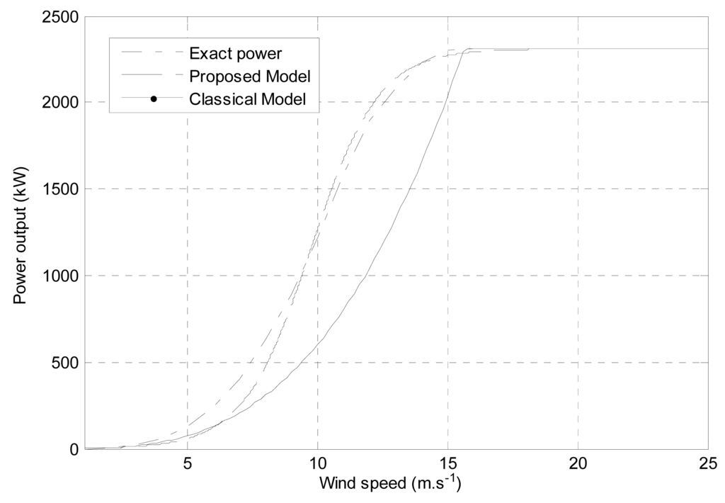
The proposed model given in Equation (10) is validated on several wind turbines (Nordex, Vestas, Enercon, etc.). Figure 2 shows the power characteristics of the ENERCON E70 wind turbine for which P_rated = 2300 kW, rated wind speed u_r = 16 m s⁻¹ and rotor radius R = 35.5 m. As it can be seen from the figure, the values of power output obtained by using the proposed model are in agreement with the exact power values of the installed WTS. The difference is very small as compared with those of classical model given in Equation (3). The model properly characterizes the variation of the power output with respect to wind speed and can be used for modeling of power curves for this type of WTSs in analyses and design optimization studies.

3.2. Computation of Rated Wind Speed

It is well-known that rated wind speed is related to the turbine rated power and its value affects the capacity factor and the amount of energy production. For a WTS, if a turbine with a higher rated wind speed is used at a site of lower wind potential, the WTS will operate at a low capacity factor and the COE will increase. On the other hand, if the turbine with a lower rated wind speed is used in a site of higher wind potential, the WTS will operate at high capacity factor for all wind speeds but only a small part of the wind energy will be converted into electrical energy at higher wind speed values. Accordingly, the rated power of a WTS, its rated wind speed and wind potential of the site must match each other to produce electrical energy at higher efficiency and lower cost. A numerical method is presented to calculate the value of rated wind speed of a WTS taking into account the wind potential of the site. The capacity factor could be easily obtained from Equations (6), (7) and (10) as follows:

$$C_f=\frac{P_o\mathit{(}{u}_o\mathit{)}}{P_{\mathit{\text{rated}}}}=\underset{u_{ci}}{\overset{u_{co}}{\int }}W\mathit{(}u\mathit{)}\frac{\mathit{1}}{\mathit{1}+e^{-\mathit{(}bu-\mathit{7}.\mathit{5}\mathit{)}}}du$$

(12)

Firstly, the value of rated wind speed with the Weibull scale parameter is determined for a given value of capacity factor ranging from 0.2 to 0.5 and for the value of the Weibull shape parameter k = 2 as in the Rayleigh distribution by using Equation (11) in Equation (12). In this case, the scale parameter of the Weibull distribution is in the range of 5–12 m s⁻¹ with the incremental step of 0.2 m s⁻¹. Figure 3 illustrates the variation of rated wind speed with scale parameter of the Weibull distribution for different values of the turbine capacity factor.

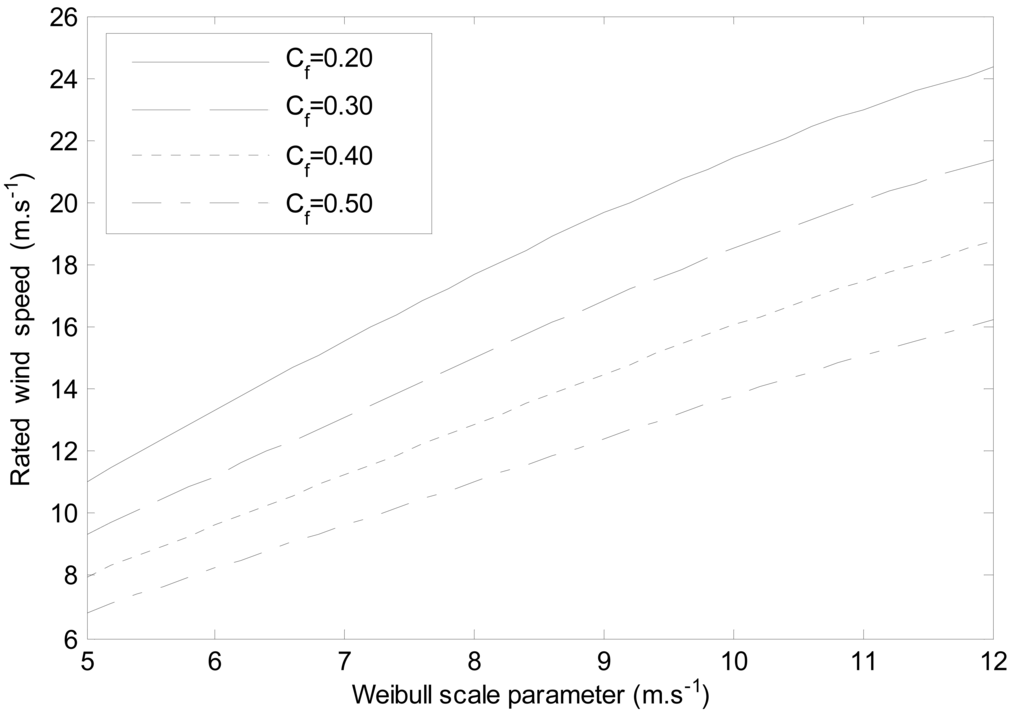
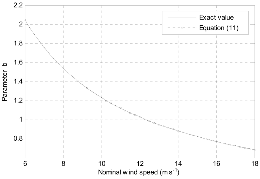
It is seen from the figure that the rated wind speed value increases with the scale parameter as expected. This relation between rated wind speed and scale parameter is defined in exponential form by using the curve fitting method [17] as follows:

$$u_r+u_1{c_w}^{u_2}+u_3$$

(13)

where c_w denotes the scale parameter of the Weibull distribution; and u₁, u₂ and u₃ are coefficients which are a function of the turbine capacity factor. These coefficients are modeled as a fourth degree of polynomial function of the capacity factor as follow:

$$u_{\mathit{1},\mathit{2},\mathit{3}}=p_{\mathit{1}}{C_f}^{\mathit{4}}+p_{\mathit{2}}{C_f}^{\mathit{3}}+p_{\mathit{3}}{C_f}^{\mathit{2}}+p_{\mathit{4}}{C}_f+p_{\mathit{5}}$$

(14)

The value of coefficients p₁–p₅ are determined for different values of the capacity factor ranging from 0.2 to 0.5 using the curve fitting method and are given in

Table 2. The value of p₁–p₅ coefficients for computing rated wind speed.

Parameters	p1	p2	p3	p4	p5
u1	4516.99681	−7626.5	4905.05453	−1440.441	167.39169
u2	−8.130122	5.4536707	−3.6212639	3.6796783	−0.281603
u3	−4654.9957	7888.3	−5149.5471	1557.1447	−188.5758

. The reliability of the proposed model given in Equations (13) and (14) is tested for different value of capacity factor and scale parameter compared with the solution of Equation (12). It was observed that the maximum absolute error in the rated wind speed is around 1.5% which can be neglected and the error decreases as the value of capacity factor increases. Accordingly, the proposed model could be successfully used to calculate the rated wind speed of variable-speed WTSs considering the wind potential of the site, which results in computation of power output with steady wind speed using the proposed model given in Equation (10).

3.3. Optimization Algorithms

The objective of this study is to optimize the design parameters to produce electrical energy at minimum cost. In order to estimate the per-COE produced by a WTS, the model developed by National Renewable Energy Laboratory (NREL) [9] is utilized. The model is based on the economy and the performance of a WTS. The COE is calculated by using the following equation:

$$\mathit{\text{COE}}=\frac{\mathit{\text{FCR}}\times \mathit{\text{ICC}}+\mathit{\text{AOE}}}{\mathit{\text{AEP}}}$$

(15)

where ICC is initial capital cost ($) consisting of the rotor components, drive train, tower cost, and the expenses of manufacturer services, etc; FCR is the fixed charge rate (1/yr); AOE is the annual operating expenses ($/yr), including land lease costs and replacement costs. For this model, an algebraic equation of all components are given in [9] in detail.

Population based optimization algorithms, namely the artificial bee colony (ABC) [18] and particle swarm optimization (PSO) [19] algorithms are used to design a WTS for a specific site. The ABC algorithm is developed based on the observation of the behavior of honey bees in their finding of nectar and sharing this information with other honey bees in the hive. In this algorithm, three groups of bees have been defined for finding a food source. These are called as employed bees, onlooker bees and scout bees. The algorithm consists of three steps which are sending the employed bees onto their food sources and evaluating their amounts of nectar; after sharing the nectar information of the food sources, the selection of new food source regions by the onlooker bees and evaluating the nectar amount of the food sources; determining the scout bees and then sending them randomly onto possible new food sources. In this algorithm, the position of a food source represents a possible solution to the optimization problem and the amount of nectar of a food source corresponds to the fitness of the associated solution. In the algorithm, the fitness of a food source is given by the value of the objective function of the problem. In order to terminate the ABC algorithm, there are three main control parameters: the number of food sources, which is equal to the number of employed or onlooker bees, the value of the fitness values between two successive iterations and the maximum number of iterations [18].

The PSO algorithm is capable of converging to a global optimum solution for all types of complex optimization problem [14,19]. The algorithm uses the procedures of moving particles around a multi-dimensional search space for approaching the optimal point. Firstly, a particle group is created randomly and put into motion. By considering its own experience and that of neighboring particles, each particle sets its movement by regulating its position. After each optimization, all particles experience the fitness value and change their position towards to a better one. Since the speed of each particle is a random variable, they can be updated depending on the distance from the best location. The velocity (v) and position (p) of each particle i is updated. The procedure in the algorithm is stopped if any one of the following two convergence criteria is satisfied. These criteria are the fitness value between two successive iterations and the maximum number of iterations [19].

The wind turbine design problem is a nonlinear and constrained optimization problem because of the complexity of systems containing multiple components. However, the ABC algorithm is a tool for optimizing unconstrained problems. In this work, it is applied to the WTS design problem by extending the basic ABC algorithm adding a constraint because it is capable of converging to a global optimum. In both algorithms, the objective function is the per-COE in $/kW h. They optimize generator power, rotor diameter, hub height and turbine capacity factor and determine the rated wind speed by taking into account the site's wind conditions to generate electrical energy at maximum efficiency and minimum cost. In order to increase reliability and computational efficiency, an empirical formula described in [20] is incorporated into the optimization algorithm as an inequality constraint with ±10% tolerances as given in Equation (16) to compute the approximate value of rotor diameter and resulting of generator power with respect to hub height:

$$D_r={\left(\frac{h}{\mathit{2.7936}}\right)}^{\frac{\mathit{1}}{\mathit{0.7663}}}$$

(16a)

$$\mathit{0.9}\times D_r\le D\le \mathit{1.1}\times D_r$$

(16b)

Geographical variables are also used as equality constraints. In order to compute the air density (ρ), the average temperature (T_o) and altitude of the site (H) are taken as an input parameter besides the value of shape and scale parameter (k, c) at reference hub height. In the optimization process, hub height, capacity factor, rotor diameter and generator power are selected as the input parameters. Additionally, rated wind speed is also another input parameter. However, it is not optimized, as it depends on hub height and the capacity factor defined by Equation (13) and it is used in the computation of rated power and the amount of produced energy using developed model. As indicated in

Table 3. Variation range of optimization parameters.

Parameter	Range of parameter	Step
Capacity factor (Cf)	0.2–0.5	Random
Hub height (h)	15–100 (m)	Random
Rotor diameter (D)	Equation (16) (m)	Random
Rated power (Prated)	Equation (1) (W)	Random (u = ur and Cp-max = 0.4–0.5)
Rated wind speed (ur)	Equations (5) and (13) (m s−1)	-

, the values of h and C_f are randomly chosen. For each value of h in the selected range, the rotor diameter is computed by Equation (16a). Then, a range is defined in terms of computed D as given in Equation (16b) and D is randomly chosen from this range. Finally, for each D and computed u_r values, the rated power is calculated by using Equation (3) in which C_p-max is randomly chosen between 0.4 and 0.5. In the optimization process, h and C_f values are updated at each iteration and the remaining ones are determined based on these updated values of parameters. The implementation of the ABC and PSO algorithms for solving the WTS design problem is given in step by step fashion as follows:

• Optimization Algorithm with ABC

  • Step 1. Input geographical variables and wind data of the region (T_o, H, α, k_o, c_o and h_o);

  • Step 2. Set the total number of bees (NP) in the colony (employed bees plus onlooker bees);

  • Step 3. Set the maximum cycle number (MCN) in order to terminate the algorithm;

  • Step 4. Generate the initial bee colony (A_ij) considering the limits as given in Table 3;

  • Step 5. Evaluate the fitness of the A_ij;

  • Step 6. Repeat;

  • Step 7. For each employed bee:

    • Produce a new solution by considering the limits as given in Table 3;

    • Calculate the fitness value of the new solution;

    • Apply greedy selection process;

  • Step 8. Calculate the probability values for the solutions;

  • Step 9. For each onlooker bee:

    • Select a solution depending on probability values;

    • Produce new solution considering the limits as given in Table 3;

    • Calculate the fitness value of the new solution;

    • Apply greedy selection process;

  • Step 10. If there is an abandoned solution then replace it with a new solution which will be randomly discovered by scouts;

  • Step 11. Save the best solution;

  • Step 12. Until cycle = MCN.

• Optimization Algorithm with PSO

  • Step 1. Input geographical variables and wind data of the region (T_o, H, α, k_o, c_o and h_o);

  • Step 2. Set the maximum number of iterations and the tolerance of fitness values;

  • Step 3. Create a “population” of agents (particles) considering the limits as given in Table 3;

  • Step 4. Evaluate each particle's position according to the objective function;

  • Step 5. If a particle's current position is better than its previous best position, update it;

  • Step 6. Determine the best particle (according to the particle's previous best positions);

  • Step 7. Update particles' velocities as follow:

    $${{\nu }_i}^{t+\mathit{1}}={{w\nu }_i}^t+c_{\mathit{1}}{\mathit{\text{rand}}}_{\mathit{1}}({{\mathit{\text{pbest}}}_i}^t-{p_i}^t)+c_{\mathit{2}}{\mathit{\text{rand}}}_{\mathit{2}}({\mathit{\text{gbest}}}^t-{p_i}^t)$$

    (17a)
    $${p_i}^{t+\mathit{1}}={p_i}^t+{{\nu }_i}^{t+\mathit{1}}$$

    (17b)

  • Step 8. Move particles to their new positions and check their limits as given in Table 3;

  • Step 9. Go to step 4 until stopping criteria are satisfied.

4. Applications

The site selection and design of wind turbines could not only reduce produced energy cost but also extend the life time of turbines, which results in increased energy production. In this study, design optimization of WTSs is performed for the Northern and especially the Mediterranean areas of Europe. This is due to the fact that Mediterranean sites have a greater wind potential than Northern Europe and in these countries environmental politics have been changed in order to increase their wind turbine parks. The Weibull probability density function is used to characterize the wind characteristics of these sites. As indicated in [10], the shape parameter ranges between 1.0 and 2.0 and the scale parameter is around 8.0 m s⁻¹ for Mediterranean sites. On the other hand, k is usually around 2.0 and c ranges between 5 m s⁻¹ and 7 m s⁻¹ in North of Europe [10]. A personal computer with a Core™ 2 Duo T6600 2.4-GHz processor and 2 GB 2.4-GHz memory is used for simulations and algorithms are coded in MATLAB. The performance of the PSO and ABC algorithms are evaluated to determine the proper algorithm by performing a number of simulations. For simulations, only population size and iteration numbers are investigated to see the effects of changes on optimal solutions. For the PSO algorithm, based on simulation results, both acceleration factors (c₁ and c₂) are set to 2.0 and the weighting factor is selected as the initial weight 0.9 and the final weight 0. The population size was varied from 10 to 100 and it should be 30. The maximum number of iterations is set to 300. For the ABC algorithm, when the colony size and/or maximum iteration number are larger, the computational time increases. It should be 14 for this type of problem; therefore, the number of employed bees would be 7. The maximum number of iteration is set to 300. The probability and the fitness value of the sources are computed as in [18]. The convergence of both algorithms is formed based on the maximum number of iterations.

Firstly, the Mediterranean area of Europe is considered and its wind potential is characterized as k = 1.2 and c = 8 m s⁻¹ at h = 30 m, and α = 0.12 [10]. Design parameters of the WTS which should be established are determined by using the two optimization algorithms given in Section 3.3. Power output and performances of optimized WTSs are computed by Equations (10), (8) and (15), respectively. Results are given in

Table 4. Design parameters and performances of optimized WTS with those of reference wind turbine systems (WTSs). AEP: annual energy production; ABC: artificial bee colony; PSO: particle swarm optimization.

Parameter	p	D (m)	Hhub (m)	ur (m s−1)	Prated (kW)	AEP (kW h)	Cost of kW h ($cent)	Turbine capacity factor	Mean power (kW/yr)
Optimized WTS with ABC	3	64.92	74.1	12.41	1745	6.72 × 106	0.0366	0.4887	789
Optimized WTS with PSO	3	64.26	73.5	12.40	1705	6.57 × 106	0.0366	0.4886	771
Optimized WTS in reference [10]	3	30	30	14	1000	2.973 × 106	0.038	0.349	349.1
WTS in reference [9]	3	70	65	11.39	1500	4.45 × 106	0.049	0.3336	522.8

with those of the WTS optimized in reference [10] for this area. It is seen from the table that rotor size, hub height and rated power for optimized wind turbines determined by using the two algorithms are higher than those of the reference wind turbine. They have nearly the same COE, but the capacity factor for optimized wind turbines is higher than that of the reference wind turbine while it produces more energy. The optimized parameters of the WTS are also in agreement with those of the WTS designed for the region for which k = 2 and c = 8.5 m s⁻¹ at height h = 50 m (in reference [9] given in fourth row of the table). Even though the WTS is not located in the region of interest, this comparison is given because the region of interest and the location of WTS have nearly the same wind characteristics. The values of the design parameters of the WTS given in [9] are very close to those of the optimized WTS, but its rated wind speed is lower than that of the optimized WTS. The amount of energy production is lower and the cost of kWh is higher than those of the optimized WTS. Thus, the WTSs optimized using the two algorithms are more advantageous than the reference wind turbines.

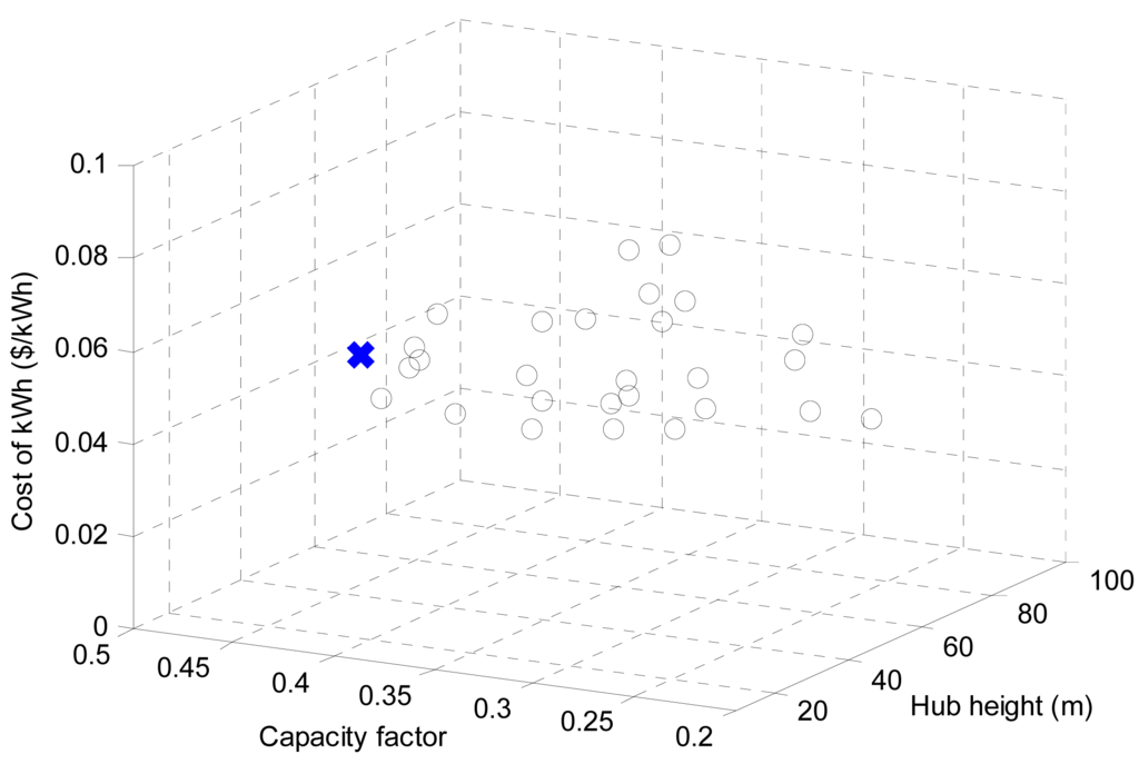
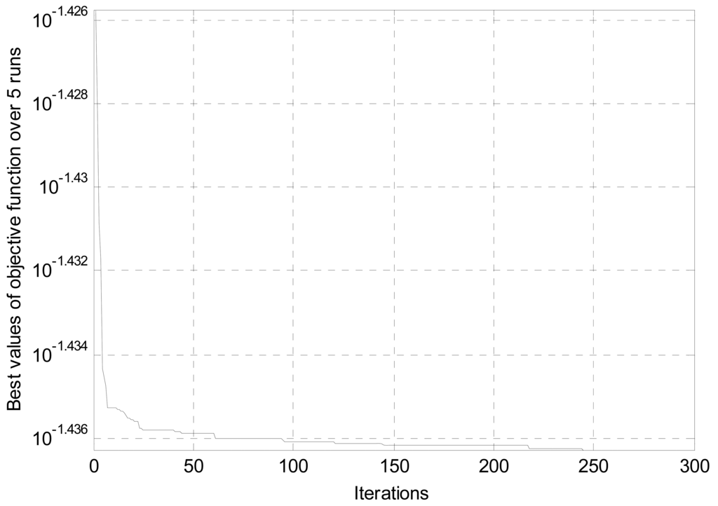
Figures 4 and 5 show initial (o) and final (x) conditions of PSO particles and variation of the best values of the objective function for the ABC algorithm, respectively. As can be seen from Table 4, both algorithms have nearly the same results. The difference between the value of the design parameter and turbine performance is too small and can be neglected. Comparatively, the performance of PSO algorithm is better than that of the ABC algorithm. However, its population size is bigger than that of the ABC algorithm. Best results was obtained with the PSO algorithm in 49.04 s; on the other hand, it was obtained with the ABC algorithm in 106 s, while the iteration number is 300.

The Northern area of Europe is also considered and its wind potential is characterized as k = 2 and c = 6 m s⁻¹ at h = 30 m, and α = 0.12 as in [10]. Design parameters of the WTS are optimized by using the PSO and ABC algorithms and results are given in

Table 5. Optimized parameters and performances of fixed-speed WTSs for Northern Europe (k = 2, c = 6 m s⁻¹ at h = 30 m and α = 0.12).

Parameter	p	D (m)	Hhub (m)	ur (m s−1)	Prated (kW)	AEP (kW h)	Cost of kW h ($cent)	Capacity factor	Mean power (kW/yr)
Optimized WTS with ABC	3	74	82	10.2	1193	4.57 × 106	0.0455	0.44	537.5
Optimized WTS with PSO	3	74	83.5	9.99	1156	4.58 × 106	0.0458	0.448	538.7

. It is seen from the table that the design parameter values obtained by the two algorithms are in close agreement. Like the first case, the performance of the PSO algorithm is better than that of the ABC algorithm for this case. Comparatively, the hub height and rotor diameter of a Northern European wind turbine are greater than those of a Mediterranean WTS, but its rated wind speed, capacity factor and rated power are small, as indicated in reference [10]. It produces low electrical energy at high cost as compared to the Mediterranean wind turbines. It is evident from Tables 4 and 5 that different wind potential leads to different design parameters and produced energy costs. Accordingly, the effect of the wind potential of regions on the produced energy cost and turbine design parameters is analyzed parametrically. The wind potential of the region is characterized by the Weibull parameters. The value of the scale parameter is changed from 5 to 10 with an incremental step of 0.2 for the fixed value of the shape parameter k = 2.

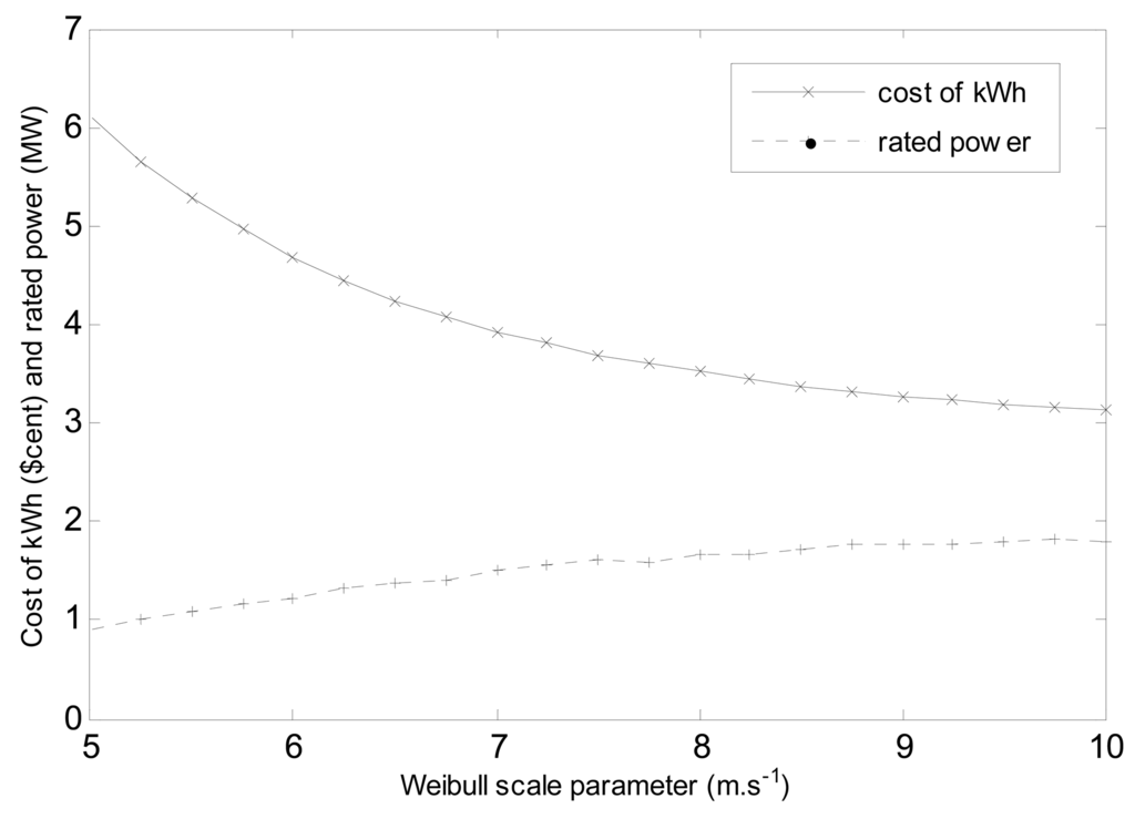
Figure 6 depicts the variation of the value of rated power and cost of kW h for optimized wind turbine with different scale parameter values. It is seen from the figure that the cost per kW h for the designed WTS decreases as the scale parameter increases. The optimized value of the rated power increases because the value of the rated wind speed increases with the scale parameter. However, the value of the rotor diameter decreases. It is also seen from the figure that the power is less dependent on the scale parameter compared to the COE. This dependency becomes the lowest as the scale parameter value increases.

For a WTS, there exists an optimum value of rated wind speed and the corresponding power is called rated power. Its value is related to the value of the design parameters (rated power and rotor diameter) and must also be compatible with the wind potential of the region. Accordingly, parametrical analyses in which the rated wind speed is changed from 8 m s⁻¹ to 18 m s⁻¹ with an incremental step of 0.25 are applied for different sites to show the effect of rated wind speed on the value of design parameters and COE as well. The value of the Weibull scale parameter is changed from 5.0 m s⁻¹ to 12.0 m s⁻¹ with the incremental step of 0.25 and optimizations are performed using the PSO algorithm given in Section 3.3. It is seen from Figure 7 that, for a given lower value of scale parameter, the value of rated wind speed has strong effect on the COE for optimized wind turbines. This effect decreases with the increase of the value of scale parameter.

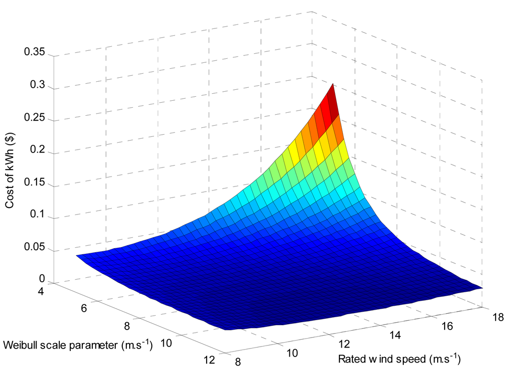
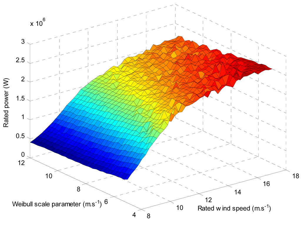
Figure 8 depicts variation of optimized value of rated power. Similar observations could be made from the figure. For a given scale parameter, the value of rated wind speed has strong effect on the rated power of WTS. On the other hand, the value of scale parameter has a slight effect on the rated power as compared with the variation of rated wind speed. It is evident from results that the rated wind speed has a strong effect on design parameters and COE. Therefore, the value of rated wind speed must be taken as an input parameter for design optimization studies.

5. Conclusions

In this study, a new method for computing turbine power output and AEP for variable-speed WTSs was proposed. The new model was developed from an S-type curve and it is only a function of the rated power and rated (nominal) wind speed. A mathematical method was also proposed to calculate the value of rated wind speed in terms of turbine capacity factor and the scale parameter of the Weibull distribution. The developed power output computation model has the advantage of having less parameters and enabling the user to calculate power output without using the rotor power coefficient as compared with the classical computation method. Additionally, the proposed approach for determining rated wind speed was also found to be reliable. It could be successfully used to calculate the rated wind speed by taking into account the wind condition of the regions in design optimization applications of variable-speed WTSs.

Secondly, a framework for design optimization of a WTS was proposed. It is based on the cost reduction by taking into account the wind characteristics and geographical features of the site. Various parameters such as rotor diameter, hub height, generator rating power, capacity factor and rated wind speed that define the configuration of a WTS were used as design parameters. In order to increase reliability and computational efficiency, an empirical formula describing relations between hub height and rotor diameter is incorporated into the optimization algorithm as an inequality constraint. The geographical and aerodynamic variables were also used as equality constraints, and the design optimizations were performed by using the PSO and ABC algorithms. The ABC algorithm was found to be efficient for such problems. However, it requires higher computational time when compared with the performance of the PSO algorithm. Different sites: Northern Europe and Mediterranean sites were considered. It was found that optimized wind turbines have an excellent profitability when compared with referenced WTSs. Parametrical analyses were also carried out in order to evaluate the effect of rated wind speed on design parameters such as turbine rated power and turbine performance. It was observed that the value of rated wind speed has a strong effect on both design parameters as well as COE for this type of WTSs and it must be taken into consideration as a key design parameter in optimization studies.

References

- Heier, S. Grid Integration of Wind Energy Conversion Systems; Wiley: New York, NY, USA, 1998. [Google Scholar]
- Sing, C. Variable speed wind turbine. Int. J. Eng. Sci. 2012, 2, 652–656. [Google Scholar]
- Li, H.; Chen, Z. Design optimization and site matching of direct-drive permanent magnet wind power generator systems. Renew. Energy 2009, 34, 1174–1185. [Google Scholar]
- Munteanu, I.; Cutululis, N.A.; Bratcu, A.I.; Ceanga, E. Optimization of variable speed wind power systems based on a LQG approach. Control Eng. Pract. 2005, 13, 903–912. [Google Scholar]
- Boukhezzar, B.; Siguerdidjane, H.; Maureen, M.H. Nonlinear control of variable-speed wind turbines for generator torque limiting and power optimization. J. Sol. Energy Eng. 2006, 128, 516–530. [Google Scholar]
- Boukhezzar, B.; Siguerdidjane, H. Nonlinear control with wind estimation of a DFIG variable speed wind turbine for power capture optimization. Energy Convers. Manag. 2009, 50, 885–892. [Google Scholar]
- Barambones, O. Sliding mode control strategy for wind turbine power maximization. Energies 2012, 5, 2310–2330. [Google Scholar]
- Song, Y.D.; Dhinakaran, B.; Bao, X.Y. Variable speed control of wind turbines using nonlinear and adaptive algorithms. J. Wind Eng. Ind. Aerodyn. 2000, 85, 293–308. [Google Scholar]
- Fingersh, L.; Hand, M.; Laxson, A. Wind Turbine Design Cost and Scaling Model; Technical Report NREL/TP-500-40566; National Renewable Energy Laboratory (NREL): Golden, CO, USA, 2006. [Google Scholar]
- Diveux, T.; Sebastian, P.; Bernard, D.; Puiggali, R.J.; Grandidier, J.Y. Horizontal axis wind turbine systems: Optimization using genetic algorithms. Wind Energy 2001, 4, 151–171. [Google Scholar]
- Fuglsang, P.; Bak, C.; Schepers, J.G.; Bulder, B.; Olesen, A.; van Rossen, R.; Cockerill, T. Site Specific Design Optimization of Wind Turbines; Technical Report JOR3-CT98-0273; National Laboratory Risø: Roskilde, Denmark, 2010. [Google Scholar]
- Collecutt, G.R.; Flay, R.G. The economic optimization of horizontal axis wind turbine design parameters. J. Wind Eng. Ind. Aerodyn. 1996, 61, 87–97. [Google Scholar]
- Fuglsang, P.; Bak, C. Site-specific design optimization of wind turbines. Wind Energy 2002, 5, 261–279. [Google Scholar]
- Kongam, C.; Nuchprayoon, S. A particle swarm optimization for wind energy control problem. Renew. Energy 2010, 35, 2431–2438. [Google Scholar]
- Fuglsang, P.; Madsen, H.A. Optimization method for wind turbine rotors. J. Wind Eng. Ind. Aerodyn. 1999, 80, 191–206. [Google Scholar]
- Maki, K.; Sbragio, R.; Vlahopoulos, N. System design of a wind turbine using a multi-level optimization approach. Renew. Energy 2012, 43, 101–110. [Google Scholar]
- Chapra, S.C.; Canale, R.P. Numerical Methods for Engineers; McGraw-Hill: New York, NY, USA, 1988. [Google Scholar]
- Karaboga, D.; Basturk, B. On the performance of artificial bee colony (ABC) algorithm. Appl. Soft Comput. 2008, 8, 687–697. [Google Scholar]
- Kennedy, J.; Eberhart, R. Particle Swarm Optimization. Proceedings of the IEEE International Conference on Neural Networks, Perth, Australia, 27 November––1 December 1995; Volume 4, pp. 1942–1948.
- Zervos, A. Wind Energy—The Facts: A Guide to the Technology, Economics and Future of Wind Power; European Wind Energy Association: Brussels: Belgium, 2009. [Google Scholar]
© 2014 by the authors; licensee MDPI, Basel, Switzerland. This article is an open access article distributed under the terms and conditions of the Creative Commons Attribution license ( http://creativecommons.org/licenses/by/3.0/).