1. Introduction
The term Smart Grid (SG) is associated with the new concept of “smart” electricity distribution networks, whose aim is the introduction of intelligence (through Information and Communications Technologies—ICT) for the optimization of the production and distribution of electricity.
In trying to meet the electricity demand with sufficient energy, utilities need to anticipate this demand by using estimate forecasts, usually 24 h ahead, and thus be able to know if they will need to buy energy in the market (energy defect), or sell it (excess energy). This is known as
Short-Term Load Forecasting (
STLF), and helps in planning the operation of generators and energy related systems owned by the utility. Nowadays, research on areas such as
Demand Response (
DR) [
1] and
Demand Dispatch (
DD) [
2] is being conducted in order to involve
SG and
STLF techniques.
As shown in [
3],
SG enables the bi-directional flow of electric energy and information between utilities and consumers. It facilitates the integration within the network of the increasingly popular renewable generation sources, by promoting the participation of end users in energy saving and cooperating with the
DR mechanism. The main objective of
DR is the reduction of peak load within its control environment, whether it is a distribution network, a
Smart City (
SC) or a
microgrid.
As shown in [
4], valley periods require the utilities to reduce the production of generators with respect to peak periods. This production adaptation is especially difficult when renewable energies enter the equation, because their output power is much more difficult to forecast.
There are two groups that use Peak Load Forecasting (PLF). Regarding to the first group, several models have been employed in the literature for PLF with different horizons. Regarding to the second group, other studies have employed PLF to facilitate STLF, since the estimation of this value becomes fundamental to improve the forecasting models.
Regarding
PLF, there have been several works reported with different horizons. Mohan and Kumar [
5] present a model based on an
Artificial Neural Network (
ANN) in order to make a
PLF of the next day and up to seven days in advance. It achieves a range of
Mean Absolute Percentage Error (
MAPE) of 1.06% to 3.39% for the next day and of 1.72% to 4.15% for a forecasting horizon of 7 days.
With regard to long-term
PLF, Hyndman and Fan [
6] show that long-term demand forecasting plays an important role for the future of production plants. Authors advocate for a probabilistic approach to long-term peak load forecasting, and to support this model, they present a methodology to forecast the probability density of long-term peak load.
McSharry
et al. [
7] study the evolution of peak load along ten years, considering the impact of calendar variables such as day of the week and month. Then they present a model using weather variables, seasonality and calendar as input data.
There have been studies of
PLF through hybrid systems, a combination of several prediction models in cascade to obtain the final estimation. The work in [
8] presents a hybrid model for
PLF of the next day, using a previous classification of similar patterns, and introducing climatic variables to improve the forecasting. To carry out the classification the
Self-Organizing Map (
SOM) model is used, and then a specialized
ANN MultiLayer Perceptron (
MLP) is applied for
PLF inside each cluster. Depending on the cluster used,
MAPEs range from 1.56% to 3.51%.
Another hybrid system is presented in [
9], which includes three different solutions for annual
PLF. In the worst case a
MAPE of 32% and in the best case of 3.7% are obtained. The work published in [
10] shows a hybrid system for
PLF of the next day. Authors propose a module for data decomposition into low and high frequency using Wavelets. The
MAPE varies from 1.2% to 1.57%.
A disadvantage of previous studies (except [
7]) is that they need lots of patterns for the learning phase. In particular, [
5] needs three years of data, [
6] uses 10 years, [
8] employs four years, [
9] needs over 15 years to obtain certain indexes that will be used in the estimation and [
10] employs five years. As for [
7], it only needs one year of data in the learning phase, but achives a
MAPE of 2.52%. The model proposed in this work, only requires two years of data, much lower values than at [
5,
6,
8,
9], and a similar values to the one used in [
7], with the difference that the
MAPE obtained with the model proposed here is 1.62%.
Some studies of the second group will be then presented. These works use
PLF as input parameter of the model which will make
STLF. Jain and Satish [
11] present a hybrid system based on statistical models and
ANN to make
STLF. This system is composed by four modules and the system uses variable load and weather.
Amral
et al. [
12] present three different models to make
STLF. The first model delivers 24 values at the same time using a
MLP. The second model delivers peak load and valley load through two
MLP, for later use them with statistical average of the load curve and to deliver the next day
STLF. The third model features 24
MLPs in parallel.
The interesting feature of [
11] lies in the synergy of models obtained from their combination, to get then a more accurate estimation through this combination. What is remarkable in [
12] is the use of peak load and valley load to subsequently, by an average of load curves, to make the next day
STLF. The model presented in this paper will be based on the potential of several stages to obtain
STLF and, in addition, in the use of characteristic parameters of the load curve, such as: two peak loads, two valley loads and aggregate demand; all of them being estimates of the next day.
Everything presented so far corresponds to environments of vast areas with high populations (for example, in reference [
5]: Haryana (India), with a population of 21 million people) and with high power consumption which will make demand habits overlap, relaxing the profiles of the load curve. The ranges of consumption of the cited publications are: 500–3500 MW [
4]; 1000–3000 MW [
6]; 1000–1800 MW [
7]; 2500–4600 MW [
8]; 1350–1800 MW [
9]; 20,000–42,000 MW [
10]; 9000–15,000 MW [
11]; and 200–400 MW [
12].
According to the
Consortium for Electric Reliability Technology Solutions (
CERTS) [
13] a
microgrid is: “(
...)
an aggregation of loads and microsources operating as a single system providing both power and heat. The majority of the microsources must be power electronic based to provide the required flexibility to insure operation as a single aggregated system. (
…)”. It seems logical to think that for the proper functioning of a
microgrid, it is essential to bear in mind demand behavior, requiring its forecasting and subsequently trying to adjust the
microgrid generation to such claim. These environments require classification algorithms and clustering of the load curves to subsequently forecast the demand, as show in [
14].
This paper presents a model based on
ANN which makes
STFL of the next day in a
microgrid environment, using variables such as input to the network and estimated values of the day intended to be forecast. These points of interest are: the two maximum values (peak load), the two minimum ones (valley load) and aggregate demand. These variables together with other variables will make the forecast fit better to the model compared to another one with data of the same location. The objective will be to achieve accurate forecasting using information of the curve to forecast. The analyzed models used the estimation of peak load and valley load of the day to forecast, but not the two peaks and two valleys of the curve to forecast. The model will be compared with reference [
15], where the location and data are the same.
There are two main differences between the method proposed along this work and other documented approaches: first, it is based on a two stage predictor, which forecasts a set of meaningful intermediate parameters (peaks and valleys in the load curve) as an input for the final prediction of the load curve; and second, it employs less data (only two years) than most of the methods reported in the literature. The paper is organized in the following way:
Section 2 presents the methodological framework and data.
Section 3 shows the structure of each of the employed
MLP.
Section 4 validates the model with real data.
Section 5 analyzes the results.
Section 6 presents the conclusions.
2. Data Description and Methodology Framework
2.1. Load Data
Iberdrola provided a historic data set from 1 January 2008 until 31 December 2010, of the capital of the province of Soria (Castilla y León, Spain), which presents one sample per hour. The consumption, characteristic of a microgrid, varies between 7–39 MW, and does not conform to the pattern of values of a country or a wide region. After deleting the existing erroneous patterns of the 3 years of available data, 70% have been used for learning (70% training ratio, 15% validation ratio and 15% test ratio) of the MLP, and the remaining 30% for the validation phase.
The meteorological data used in this study were collected by the Spanish Meteorological Agency AEMET from the meteorological station installed in Soria. The meteorological data were collected from 1 January 2008 to 12 October 2010. The weather variables considered are: precipitation (mm), air temperature (°C), average wind speed (m/s), average wind direction (sexagesimal degrees), relative humidity (%), pressure (hPa) and global solar radiation.
Each row presents data about date and hour of registration, minute of registration, source meteorological station, altitude, name of the province, longitude, latitude, precipitation, ambient temperature, average wind speed, average wind direction, relative humidity, pressure and global solar radiation. Weather variables—excluding global solar radiation, which is sampled hourly between 5:00 and 20:00—are monitored on a ten-minute basis. Missing values due to monitoring failures are recovered using interpolation (this is done to implement a system capable of working in real time). Then, air temperature, average wind speed, average wind direction, relative humidity and pressure are averaged in groups of six ten-minute intervals to obtain hourly measures. Precipitations are not averaged, but accumulated instead. Then, daily average values are calculated for all of the variables.
Microgrids must be capable of managing electric energy consumptions ranging between ten of kW to hundreds of MW. These consumptions are characteristic of small and medium sized cities, towns or even smaller environments. Behavioral habits of these locations will make the load curves show the uneven and rough environments each hour, in contrast to those shown in more aggregated environments (large areas or countries with high density and very concentrated population and high electricity consumption) because in those areas the superposition of habits, and therefore the load curves, soften the final load curve.
The hypothesis of this paper is that load curves have a very specific topology that contains a series of concepts (daily aggregate demand, two peak loads and two valley loads) that would be very important to know a priori because it would greatly facilitate the work of the predictor and improve their results. These peaks and valleys of the next day, obviously not available a priori, can be forecasted in a first stage (using predictors specialized in this type of forecasting), and then supply these forecasts to a second stage of forecasting, which will be responsible for predicting the load curve of the next day (STLF).
In this way, although the input data are the same in the case of the proposed two-stage predictor that in a direct predictor [
15], the additional variables and the ability of the first stage (forecasting of peaks, forecasting of valleys and forecasting of daily aggregate demand) will improve the performance of the global system.
2.2. Methodology Framework
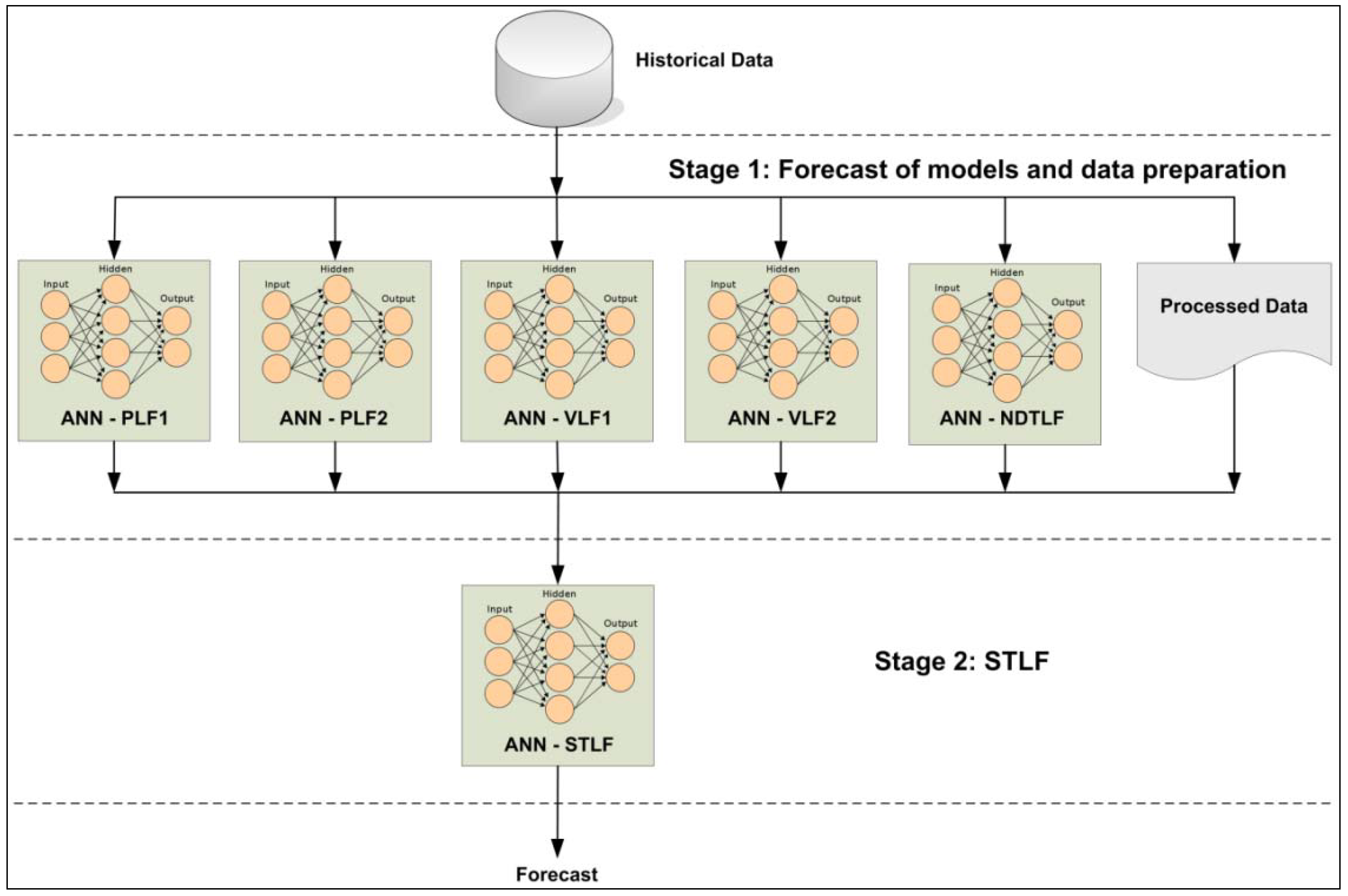
This paper presents a methodology for
STLF through input variables based on estimated details of the forecasting day. The methodological framework (
Figure 1) can be summarized in two stages: forecast of models and data preparation; and
STLFs of the next day.
Figure 1.
Block diagram of the proposed methodology.
Figure 1.
Block diagram of the proposed methodology.
All data mentioned in
Section 2.1 are stored in a database, which will be connected with the first stage of the submitted methodological framework. Six different actions will be carried out at this early stage:
ANN-PLF1: MLP network, it is responsible for the estimation of the first peak load of the day to forecast. This network will receive the input variables of the database and will present its estimation to the second stage;
ANN-PLF2: MLP network, it is responsible for the estimation of the second peak load of the day to forecast. This network will receive the input variables of the database and will present its estimation to the second stage;
ANN-VLF1: MLP network, it is responsible for the estimation of the first valley load of the day to forecast. This network will receive the input variables of the database and will present its estimation to the second stage;
ANN-VLF2: MLP network, it is responsible for the estimation of the second valley load of the day to forecast. This network will receive the input variables of the database and will present its estimation to the second stage;
ANN-NDTLF: MLP network, it is responsible for the estimation Next Day’s Total Load (NDTL). This network will receive the input variables of the database and will present its estimation to the second stage;
Processed data: it is responsible for processing the data from the database expected as input variables by the STLF of the second stage.
The second stage will consist in an MLP network to make the next day STLF (ANN-STLF). The network will need data from the first stage to be used as input variables. Once submitted these variables, the network will deliver the estimation of the 24 values of electric energy demand of the next day.
3. ANN Structure and Evaluating the Performance of ANN
Below each of the networks used in
Section 2.2 is explained. Each of the layers (input, output and hidden) will be presented, and the variables of the input layer, the number of neurons in the hidden layer and the variables of the output layer indicated.
The way to optimize the MLPs—both to determine the number of neurons in the hidden layer and to establish the best learning algorithm—is usually performed by a heuristic method. Therefore, an automatic script developed in MatLab will be used, where all possible parameters (number of neurons in the hidden layer, learning function, network performance function during learning, etc.) will be varied to select the best topology for each of the proposed networks. For each of the models, for each of the training functions, and for each hidden layer size (between one and 20 neurons), the script executed 100 different runs in order to achieve statistically meaningful results which rule out the random factors influencing the ANN (such as the initial state). The training functions considered are: traingd is gradient descent backpropagation; traingdm is gradient descent with momentum backpropagation; traingda is gradient descent with adaptive learning rate backpropagation; traingdx is gradient descent with momentum and adaptive learning rate backpropagation; trainrp is resilient backpropagation; traincgf is conjugate gradient backpropagation with Fletcher-Reeves updates; traincgp is conjugate gradient backpropagation with Fletcher-Ribiére updates; traincgb is conjugate gradient backpropagation with Powell-Beale restarts; trainscg is scaled conjugated gradient backpropagation; trainbfg is BFGS quasi-Newton backpropagation; trainoss is one-step secant backpropagation; trainlm is Levenberg-Marquardt backpropagation; and trainbr is Bayesian regulation backpropagation.
The number of neurons in the hidden layer is detailed in the following sections of this paper, while the rest of parameters for all networks are common: learning function trainbr (Bayesian Regulation Backpropagation) and network performance function Sum Squared Error (SSE).
Periodic/cyclical variables, such as day of the week and month (which are essential for the
ANN to properly detect weekly, monthly and seasonal patterns), are supplied to the networks in the form of values of sines and cosines, as it has been demonstrated [
16,
17] that this transformation significantly improves the performance of the
ANN.
3.1. ANN–PLFx Structure
The presented structure serves both for
ANN-PLF1 and
ANN-PLF2, the only difference is that the network will use values from the first peak load when it is 1 or from the second peak load when it is 2. As reference of the network, results of [
18] have been used, showing a network for
PLF with a
MAPE of 1.57% and two hidden layers. It has been taken into account [
11] for selecting additional input variables.
Input: 9
PLi(d−1), PLi(d−2), PLi(d−3), PLi(d−4), PLi(d−5), PLi(d−6), PLi(d−7): peak load of the 7 previous days of the day to forecast; i is 1 or 2;
PLT(d−1): peak load temperature of the previous day of the day to forecast;
AvgT(d−1): mean temperature of the previous day to forecast.
Hidden: three neurons.
3.2. ANN–VLFx Structure
The presented structure serves both for ANN-VLF1 and ANN-VLF2, the only difference is that the network will use values from the first peak load when it is 1 or from the second peak load when it is 2. The same philosophy that ANN-PLF is followed to make the network design.
Input: 9
VLi(d−1), VLi(d−2), VLi(d−3), VLi(d−4), VLi(d−5), VLi(d−6), VLi(d−7): valley load of the 7 previous days of the day to forecast; i is 1 or 2;
VLT(d−1): valley load temperature of the previous day of the day to forecast;
AvgT(d−1): mean temperature of the previous day to forecast.
Hidden: three neurons.
3.3. ANN–NDTLF Structure
Below it is shown the
ANN-NDTLF network structure, indicating each of the variables used, both for the input layer and the output layer. Results obtained from [
19] have been used as a reference of the network. In [
19], after an analysis of the influence of climatic variables on aggregate demand, and the influence of aggregate demand regarding herself in previous days, multiple networks with different inputs are analyzed. The network with the best results is
Forecast with Aggregated Load-Working/non-working day-Day of the Week-Solar Radiation (
FALWDWSR), with a
MAPE of 2.98%.
Input: 24
TL(d−1), TL(d−7), TL(d−14), TL(d−21): the total load of a day is clearly linked with the total load of the previous day and total loads of the same day of the week of the three previous weeks, regardless of the type of day, in terms of working/non-working day and day of the week. For this reason, network inputs of the previous day and of the three similar days regarding the day of the week of the three previous weeks, have been selected as total loads;
W(d−1), W(d−7), W(d−14), W(d−21), Wd: working/non-working day (holiday = 1 and working-day = 2) of the days mentioned in the previous paragraph, as well as the working/non-working day of the day to forecast. The coding is (holiday = 1 and working-day = 2);
DW(d−1), DW(d−7), DW(d−14), DW(d−21), DWd: day of the week in sine and cosine form, both of the last days mentioned in the first point, as of the day to forecast. The coding is (Sunday = 0, Monday = 1,…, Friday = 5, Saturday = 6);
SW(d−1), SW(d−7), SW(d−14), SW(d−21), SWd: solar radiation of the last days referred to in the first point, as well as the day to forecast.
Hidden: four neurons.
3.4. ANN–STLF Structure
Below it is shown the ANN–STLF structure, indicating each of the used variables, both for the input layer and the output layer.
Input: 33
L(d−1)1, L(d−1)2, L(d−1)3, L(d−1)24: corresponding to the 24 values of the load curve of the previous day of the day to forecast;
Day of the week d − 1: this variable is introduced as two, in sines and cosines form, through sin[(2 ⋅ π ⋅ day) / 7 ](d−1) and cos[(2 ⋅ π ⋅ day) / 7 ](d−1), with day values from 0 to 6 (Sunday = 0, Monday = 1, Tuesday = 2, Wednesday = 3, Thursday = 4, Friday = 5, Saturday = 6);
Month d − 1: this variable is introduced as two, in sines and cosines form, through sin[(2 ⋅ π ⋅ month) / 12 ](d−1) and cos[(2 ⋅ π ⋅ month) / 12 ](d−1), with month values from 1 to 12 (January = 1, February = 2, March = 3,…, December = 12);
PL1d y PL2d: two maximum values of the load curve of the day to forecast (peak load 1 and peak load 2);
VL1d y VL2d: two minimum values of the load curve of the day to forecast (valley load 1 and valley load 2);
NDTLd.
Output: 24
L(d)1, L(d)2, L(d)3,…,L(d)24: corresponding to the 24 values of the load charge of the day to forecast.
Hidden: 22 neurons.
6. Conclusions
Imagine a
microgrid that has a base generation plant (hydraulic microturbine); in order to carry out peak shaving, knowledge of the peak load will be necessary so as to know the amount of water to be used the next day. As another example,
Virtual Power Plants (
VPPs) pose a challenge for demand forecasting and generation, and a possible approach is to use a management model which takes into account the multiple elements that are part of it, making them cooperate to obtain a demand forecast via
ANN in disaggregated environments, as shown by Hernández
et al. [
20].
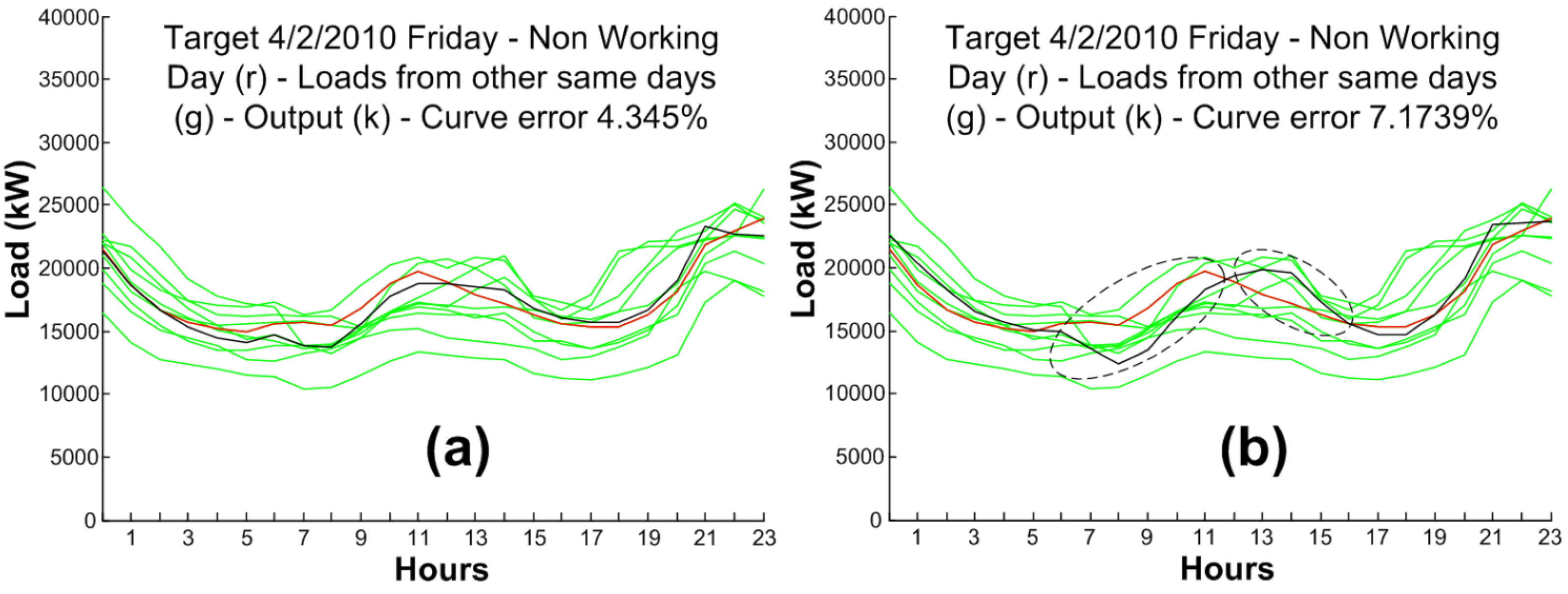
The main contribution of this paper is demonstrating that for each particular load forecast scenario a specific analysis of the influencing factors and a two stage predictor (to forecast those intermediate factors) has the potential to give better results than directly forecasting the variables of interest. In the use case presented along this work, an intermediate estimation of peak and valley values offers results that are 52% more accurate than a direct, one-stage prediction of the next day hourly load curve.
Furthermore, the test has been made with disaggregated environment data, where the zones near to the characteristic points are rougher than in more aggregated environments (large areas or countries). The deployment of microgrids is an imminent issue, so it will require its control and operation. As for consumption, a disaggregation of the load curve occurs, complicating the forecasting. In addition, there is a difficulty in demand forecasting. In addition, microgrid environments are ideal to make DR. DR is not conceived without having the most exact possible knowledge of the demand; therefore, the development of models based on ANN for STLF will be necessary, with much room for development and improvement.
With the model here presented, the forecast errors obtained for peaks and valleys are: 2.03%–2.99% (
PLF1), 2.04%–2.67% (
PLF2), 1.92%–2.22% (
VLF1), 1.88%–2.10% (
VLF2) and 1.20%–4.86% (
NDTLF). The results of valley load estimation are good and they are compared with the figures reported in [
6] (1.56%–3.51%). Valley estimation shows better results than peak estimation, mainly due to the fact that peak height and location has a greater variance than valleys. The
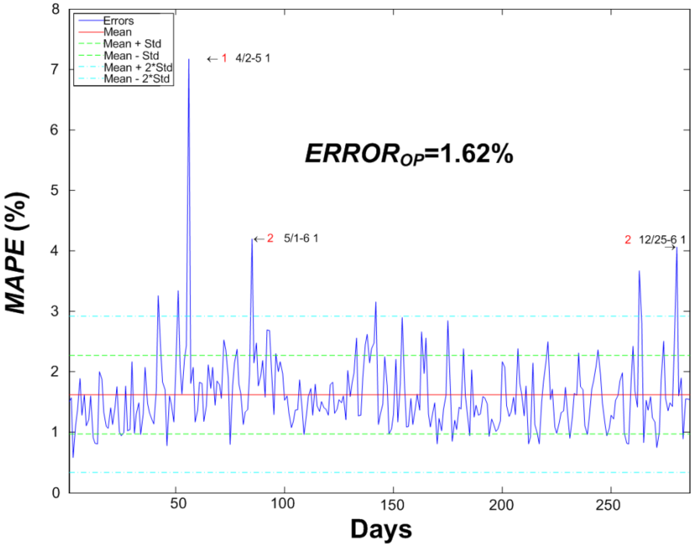
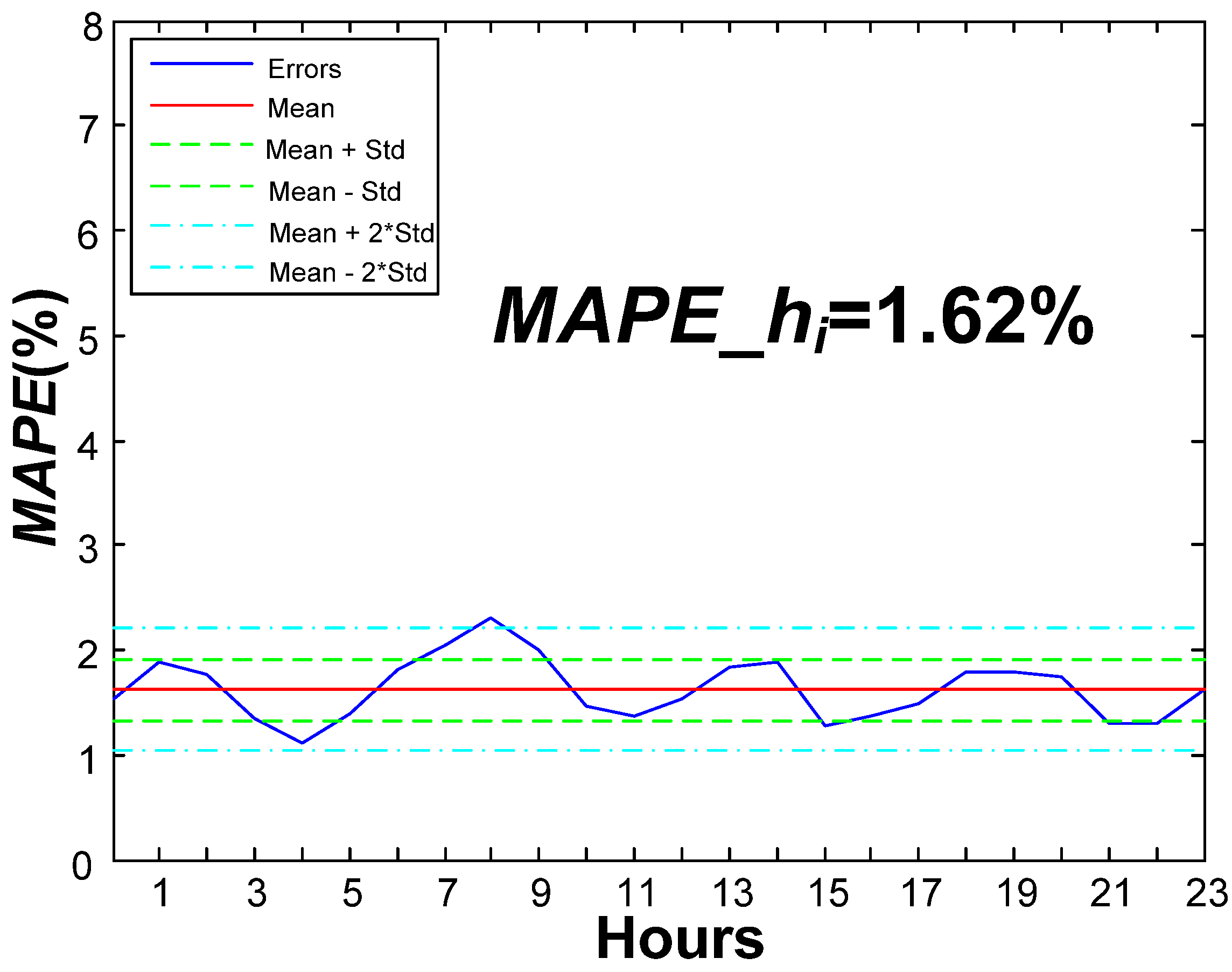
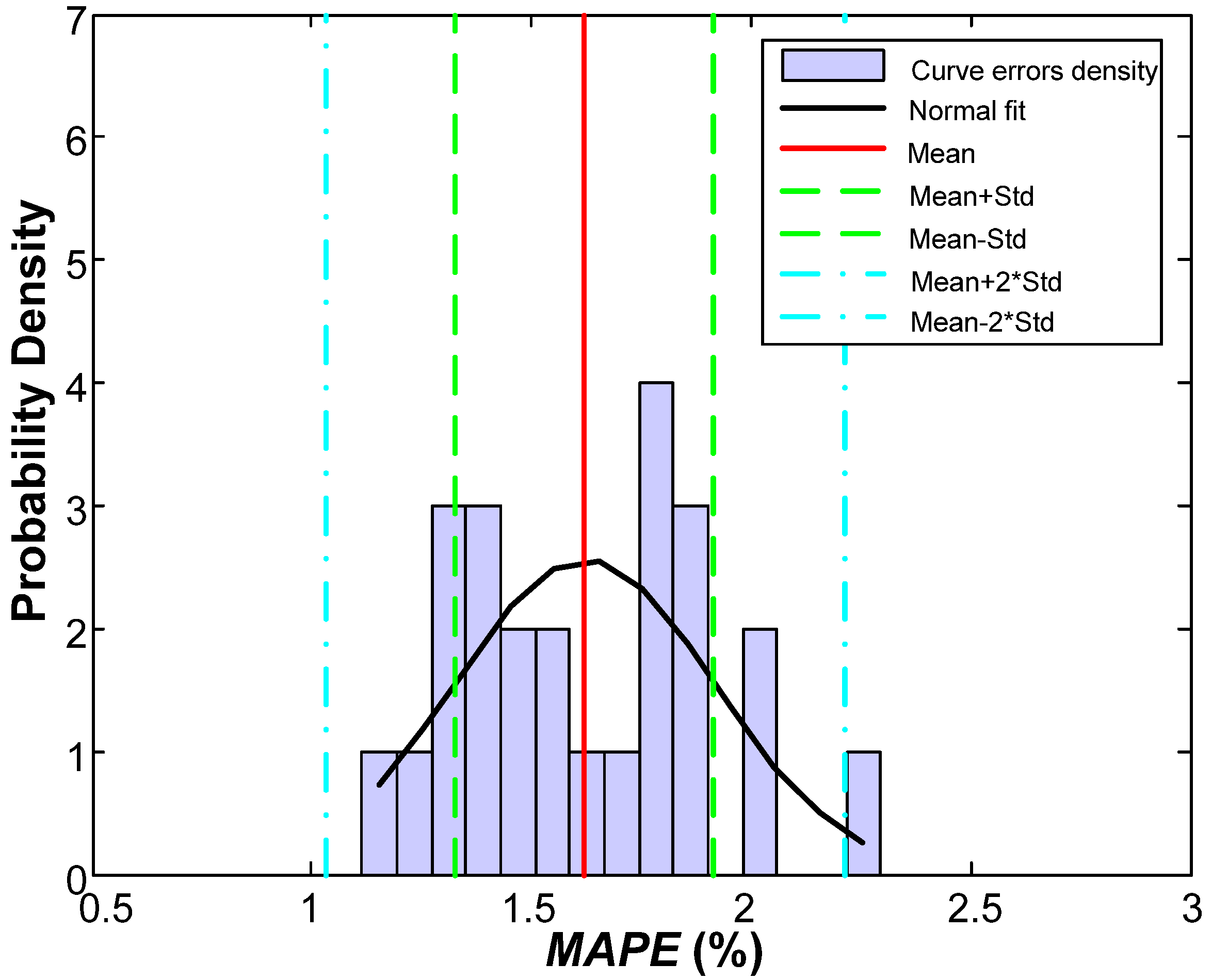
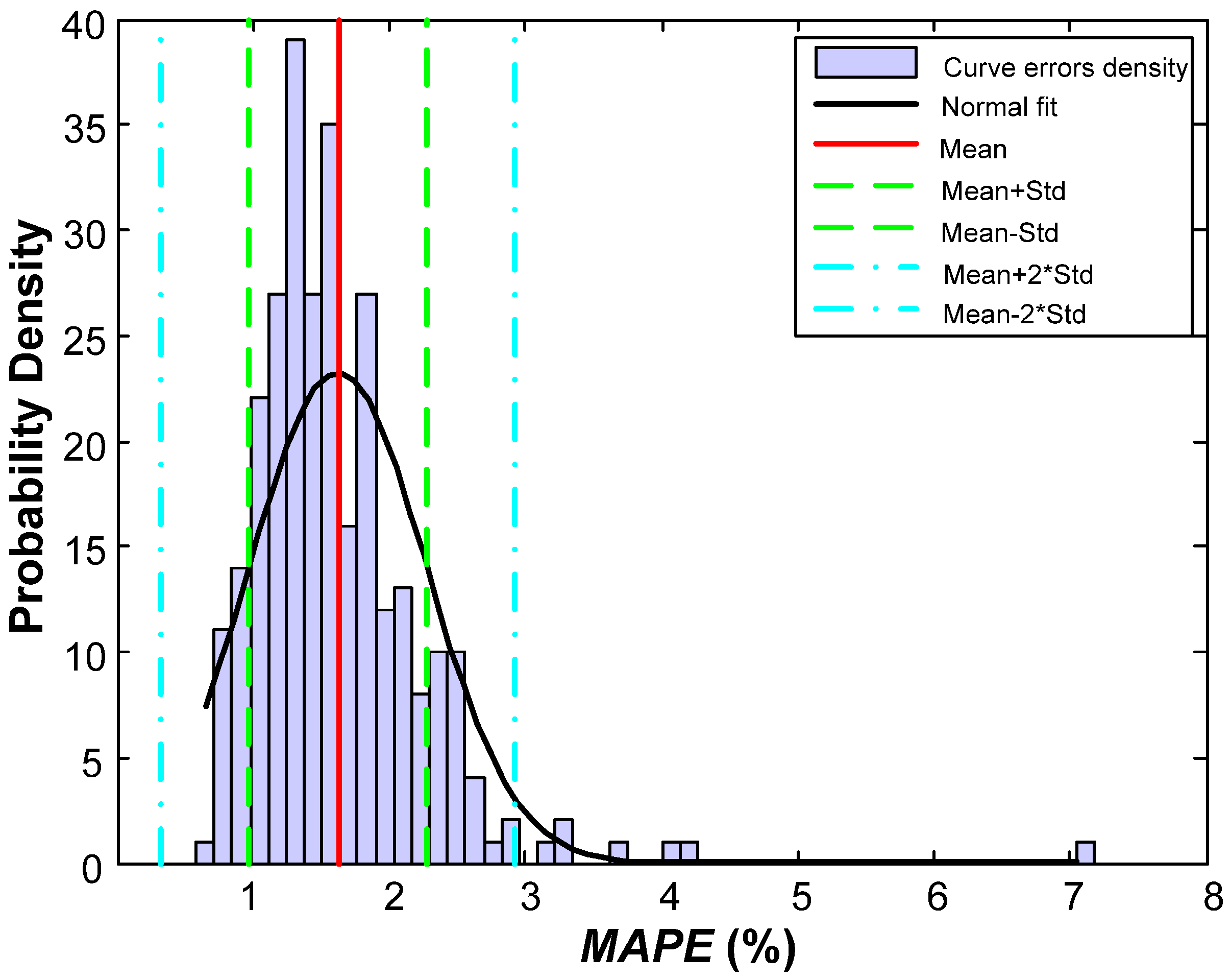
MAPE of the validation phase is 1.62%, substantially better than the one obtained in previous works (2.47%) for the same set of data. A raw improvement of 0.85% in
MAPE is a great advance, representing an overall relative improvement of 52%.


