1. Introduction
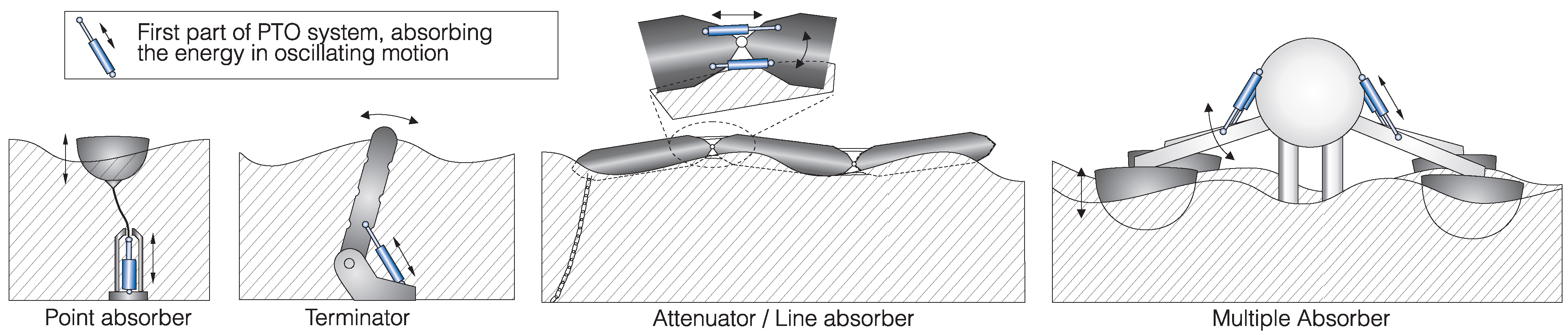
A large group of Wave Energy Converter (WEC) concepts are based on extracting energy from ocean waves using the principle of placing buoyant bodies in the sea. As waves pass the bodies, these are forced to oscillate. This is illustrated in
Figure 1, showing different version of such WECs; see [
1,
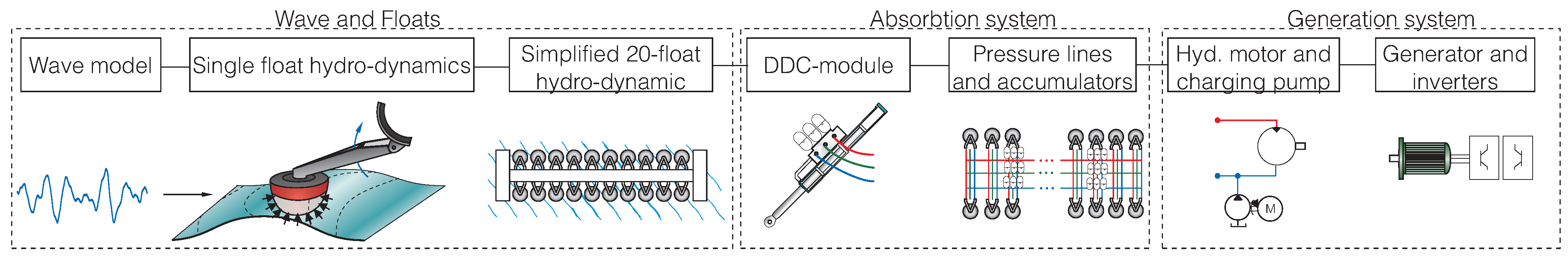
2] for a survey. The body movements are converted into electricity by a system called the Power Take-Off (PTO); see
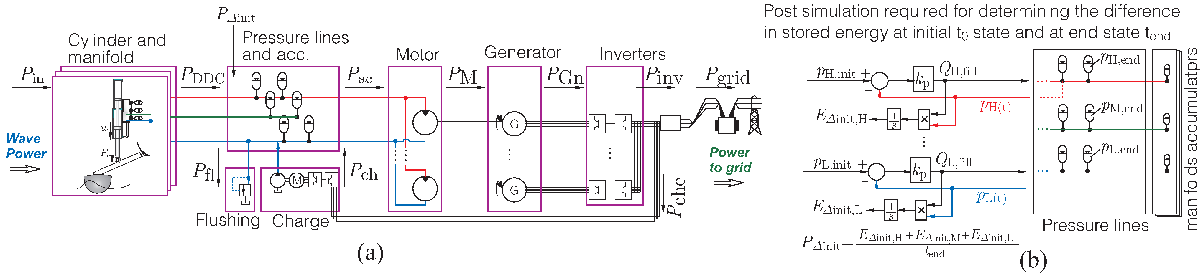
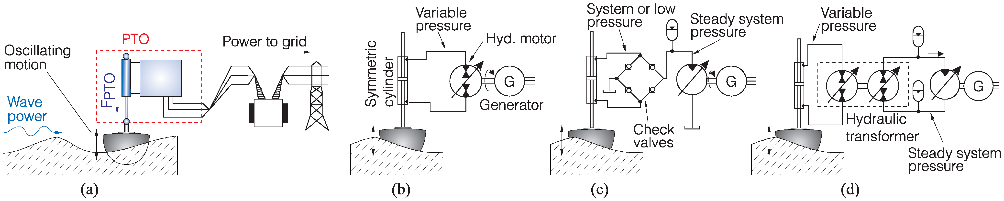
Figure 2a or
Figure 3a.
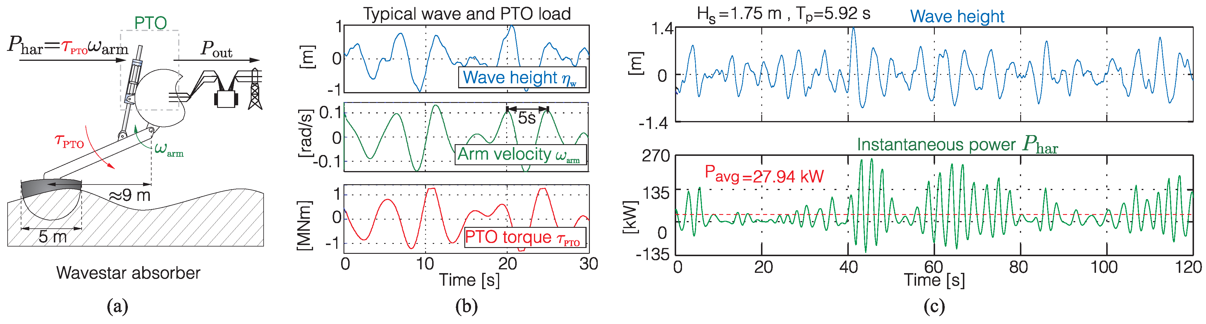
The development of an efficient and reliable PTO system is a main challenge for WECs. The problem faced is that the movement or oscillations of bodies caused by sea waves are very slow, bidirectional and irregular. An example is given in
Figure 2a, showing the resulting velocities of a 5 m diameter point absorber from the Wavestar concept. The torque,
, is the load torque applied by the PTO in order to extract energy from the absorber’s pivoting motion. The graphs in
Figure 2b shows the slow oscillation (≈5
period), resulting in a requirement of a 1 MNm bi-directional load torque for extracting an average of 27 kW. In comparison, a wind turbine operating at approximately 13 RPM would produce 1.4 MW when loading the main rotor shaft with 1 MNm. Hence, the torque density requirement for wave power is immense. Furthermore, the incoming wave power is characterized by having more than a factor of 10 between mean and peak power, as seen in
Figure 2c. The peak contributes heavily to the overall production [
3] and may not simply be discarded.
Figure 2c also shows that the energy is grouped. Resultantly, energy storage is required to store the energy peaks and use them for maintaining production between wave groups.
Figure 1.
Different embodiments of Wave Energy Converters (WECs), capturing wave energy using buoyant oscillating bodies.
Figure 1.
Different embodiments of Wave Energy Converters (WECs), capturing wave energy using buoyant oscillating bodies.
Figure 2.
(a) a Wavestar absorber; (b) velocities and PTO load in typical production waves; and (c), instantaneous power during two minutes production for a single absorber.
Figure 2.
(a) a Wavestar absorber; (b) velocities and PTO load in typical production waves; and (c), instantaneous power during two minutes production for a single absorber.
Figure 3.
(a) the definition of Power Take-Off (PTO) system; (b–d), different fluid power based transmission in PTO systems.
Figure 3.
(a) the definition of Power Take-Off (PTO) system; (b–d), different fluid power based transmission in PTO systems.
To incorporate this, power absorption requires a PTO having a complex transmission with a very high gearing ratio in order to make ocean waves power a generator. Moreover, to extract adequate amounts of energy from waves, the PTO load force,
, or torque,
, as in
Figure 2b, applied by the PTO should be controlled as a function of incident wave and body movement. Finally, to fully maximize energy extraction, the PTO should be able to operate in four quadrant mode. Four quadrant mode means that all four combination of force and velocity direction should be provided, as the PTO sometimes is required to aid the float motion (reactive control strategies). An overview of required PTO characteristics are well described in [
3].
The controllability and four quadrant behavior is required to compensate for the inherit off-resonance behavior of point absorbers. Frequency-wise, point absorbers are characterized by being narrow-banded with an under-damped resonance. To correct this deficiency, the force or torque,
, applied by the PTO to the absorber is controlled as a feedback of the absorber’s motion, allowing the PTO to adjust the absorber’s resonance frequency to match the wave frequency [
4,
5]. Optimal energy transfer from wave to an absorber is obtained when the incident wave frequency matches the resonance frequency of the absorber.
Regarding implementation of PTO systems for wave energy, several investigations have been performed on using linear generators driven directly by the absorbers’ movement. However, due to the slow linear velocities (peak linear velocity about 2 m/s), conventional permanent magnet linear generators would become very large. Typical achievable air-gap sheer-stress levels between stator and translator is about 20–25 kN/m
2 [
6]. Resultantly, a linear generator for a Wavestar float of 5 m diameter, requiring a load force of 400 kN, would be equivalent to a generator with 16–20 m
2 of active air-gap surface. In [
7], the weight of active magnetic material alone (copper, iron laminations, magnets and back-iron) is estimated to be 1500 kg/m
2. Neglecting the required support structure, the material requirements still is 24–30 tons, rendering the solution infeasible. Resultantly, effort is put into using a transmission combined with more conventional generators. Mechanical transmissions have been explored. However, these would be too massive, as a gearing ratio, which is a factor of 10 higher than a wind turbine transmission, is required, along with handling a bidirectional input.
Fluid power is a suitable technology for implementing the required transmission, as it is capable of producing high controllable forces at low velocities and easily “rectify” the bidirectional movement with compact actuators (cylinders). Unfortunately, fluid power systems are often characterized by poor efficiencies when operating at part load, which is crucial with the high ratio between peak and mean power in wave energy.
A conventional hydraulic transmission for wave energy is seen in
Figure 3b, where a cylinder operates as a pump, producing a bi-directional flow, which drives a hydraulic motor. The motor adapts to the flow and rectifies the flow into a unidirectional turning of the generator. However, an optimization of such a PTO from wave-to-grid is performed in [
8] for the Wavestar converter, showing an overall PTO power conversion efficiency below 65% at the optimum point, quickly dropping to 45% in smaller waves. The system in
Figure 3b also has the shortcoming of not allowing energy storage/smoothing.
PTO systems with the cylinder operating as a passive pump against a steady pressure, as in
Figure 3c, have been used in [
9,
10], where energy smoothing may be performed using hydraulic accumulators. This allows operating the hydraulic motor and generator at a fairly constant load, yielding a PTO efficiency of up to 80%. However, the cylinder is limited to providing a Coulomb-like force load, reducing the amount of absorbed energy [
11].
If the active valves are used instead of the passive check valves in
Figure 3c, the absorber motion may be controlled though latching to improve energy capture [
12]. The latching control prolongs the natural period of the absorber motion non-linearly by locking the absorber’s movement in parts of an oscillation cycle. This may be implemented by closing the valves, blocking the cylinder and absorber motion. This may yield the same or higher energy extraction as a load force controlled as a linear damper. In [
13], it is suggested that the energy capture of
Figure 3c may be increased by modifying with an extra accumulator with a controllable on/off valve. By, in turn, storing and releasing energy from the accumulator, the motion amplitude of the absorber may be improved.
In
Figure 3c, a PTO is shown based on a hydraulic transformer [
14], capable of controlling the force of the cylinder, while having a fixed system pressure with energy smoothing accumulators. However, the part load efficiency of the hydraulic transformer is poor, as it is basically two variable displacement pump/motors back-to-back.
It would be desirable to combine the positive features of the above system characteristics,
i.e., having a PTO with a common fixed pressure system with accumulators for energy smoothing, combined with an efficient force control of the cylinders. This has been investigated for the Wavestar system in [
15,
16], where the force control of a hydraulic cylinder is based on connecting the chambers to different fixed system pressures using an arrangement of on/off vales, as shown in
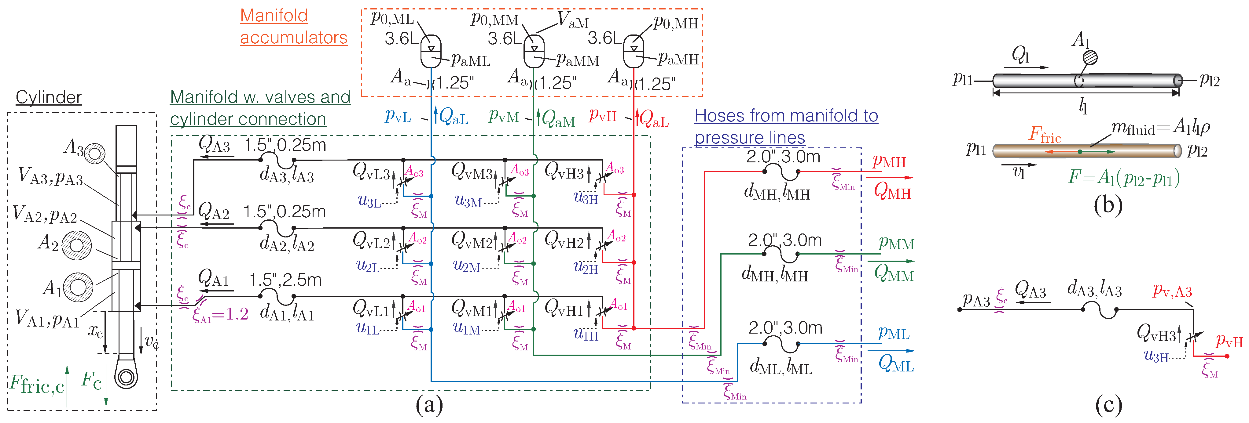
Figure 4a.
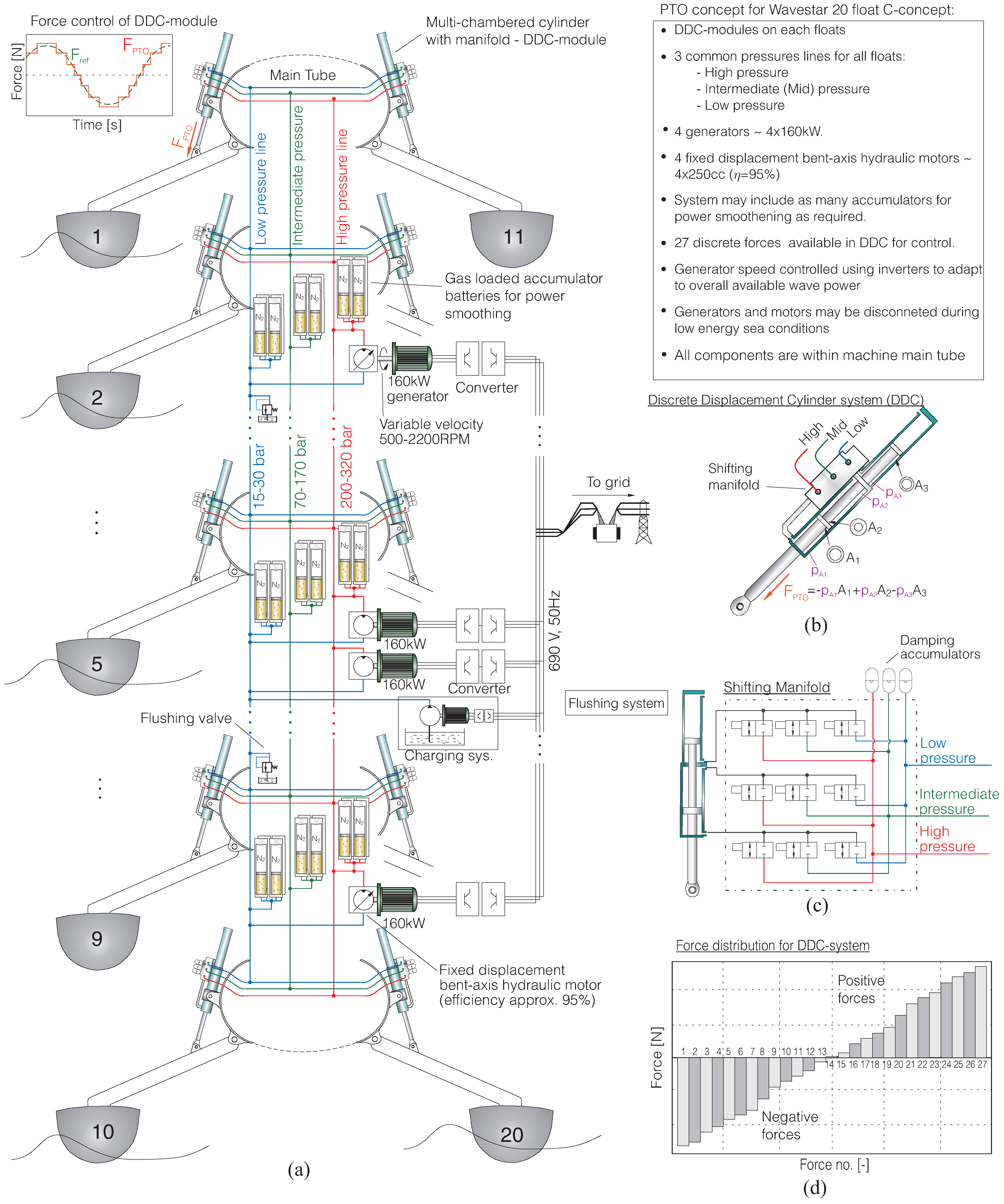
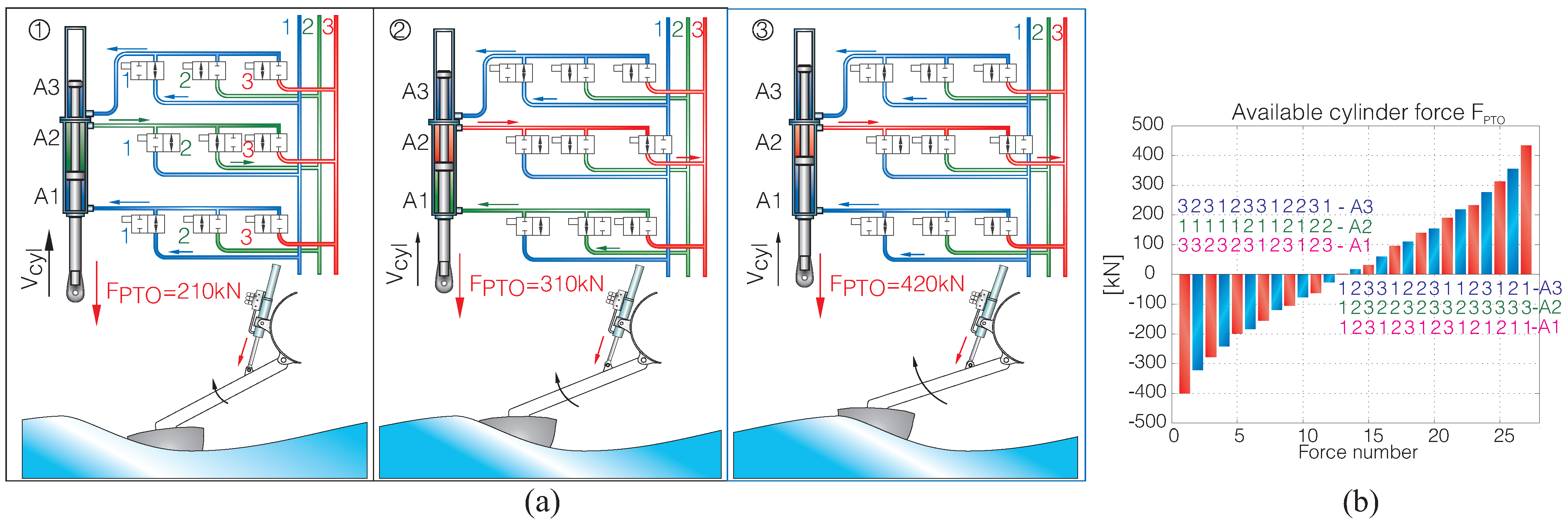
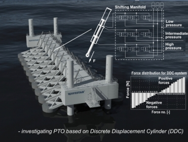
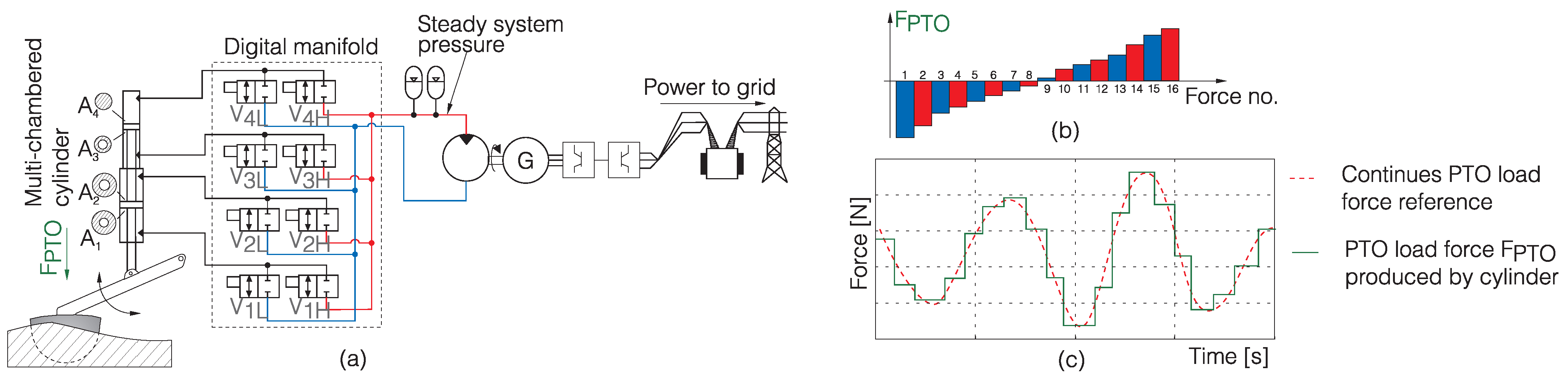
In
Figure 4a, a cylinder with four chambers is attached to a manifold with eight on/off valves. By either having system pressure (red) or low pressure (blue) in the chambers, 16 different pressure and chamber combinations are achievable for this particular embodiment, yielding 16 different available PTO forces, as shown in
Figure 4b. This corresponds to having 16 different gears available. Thus, during a wave, the PTO force is varied discretely, as shown in
Figure 4c, by shifting “gear” every half second, thereby approximating a continuous force reference. The resulting PTO force,
, is generated as the sum of forces produced by the different cylinder chambers:
As the “gear” shifting is actually a discrete variation of the cylinder displacements using the valve system, the cylinder with manifold is referred to as a Discrete Displacement Cylinder (DDC).
Figure 4.
(a) the discrete PTO system based on discrete displacement control of a multi-chambered cylinder (Discrete Displacement Cylinder (DDC)-system); (b) the forces, , the PTO may produce; and (c) how is discretely varied using the DDC-system during a wave.
Figure 4.
(a) the discrete PTO system based on discrete displacement control of a multi-chambered cylinder (Discrete Displacement Cylinder (DDC)-system); (b) the forces, , the PTO may produce; and (c) how is discretely varied using the DDC-system during a wave.
In [
15], it was shown that despite assuming infinite fast and large switching valves, a certain amount of energy will always be lost when shifting force due to the compressibility of the fluid. To assess whether a PTO system may be feasible with this unavoidable compression loss, an estimate of the PTO efficiency was calculated for the Wavestar WEC in [
15]. This was performed for different wave conditions, showing that an efficiency above 90% was reachable for the DDC. In [
16], it was shown that if the opening and closing time of the valves was kept less than 15 ms, the minimum loss could almost be assumed, thereby making the DDC feasible for a PTO solution.
Discrete control of a hydraulic cylinder has also been investigated for mobile hydraulics in [
17], showing promising energy saving compared to, e.g., conventional load sensing systems. A PTO system with a similar approach, utilizing two asymmetric cylinders has previously been discussed in [
18]. The efficiency of controlling the force of the cylinders by pressure shifting was found to be between 88% and 94%, excluding the friction of the cylinder. Currently, [
19] has shown a hydraulic transmission with accumulators for power smoothing operating at 70% efficiency. A similar system as in [
18] is suggested in [
20]. The system of [
20] is tested in a scaled version in [
21], capable of applying a torque of 16 kNm. The PTO is tested in a test-rig, simulating regular waves. The overall efficiency is estimated to be from 69% to 80%. Estimates were given, as the test-rig was not fully operational.
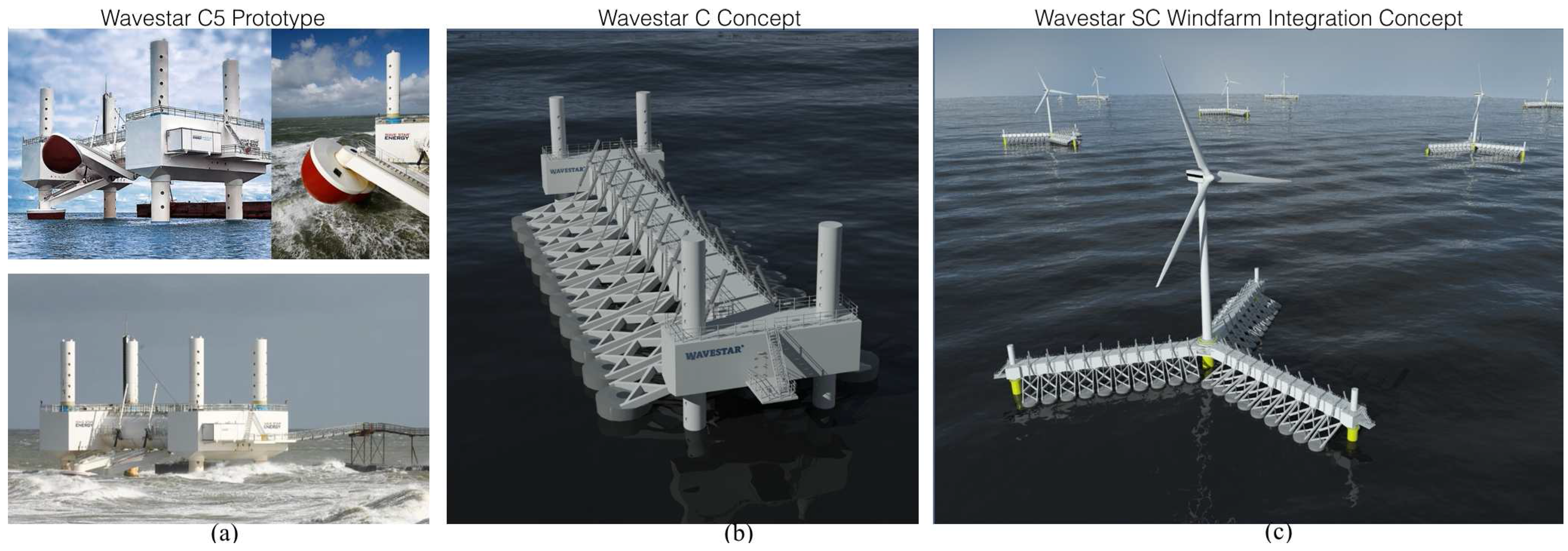
Figure 5.
(
a) full-scale Wavestar C5 prototype with two floats [
22]; (
b) Wavestar C-concept with 20 floats total; (
c) Wavestar SC-concept integration with wind turbine.
Figure 5.
(
a) full-scale Wavestar C5 prototype with two floats [
22]; (
b) Wavestar C-concept with 20 floats total; (
c) Wavestar SC-concept integration with wind turbine.
The PTO system presented in this paper is based on the results in [
15,
16] and is a complete PTO for the 20 float Wavestar C-concept shown in
Figure 5b with 5 m diameter floats. The C-concept consists of semi-submerged hemisphere-shaped floats mounted on separate arms. Each arm is mounted and rotationally supported by a common platform, which is resting on the sea bed through a number of piles. One advantage of a multiple point absorber is the increased power smoothing achieved when the waves passes through the systems. The PTO components are mainly enclosed within the main structure; only the cylinder is mounted externally. The PTO is based on a hydraulic transmission, using a fluid that is biodegradable in the marine environment. For all components inside the structure, an extra level of protection is provided, such that in the rare case of leakage, the fluid is contained inside the WEC. For the cylinder outside the machine, a sump is mounted below the cylinder, connected to automated suction lines from inside the WEC. In case of registering oil in the sump, the cylinder and float is lifted into storm protection and taken out of service until maintenance.
For storm protection and extreme seas, the Wavestar concept incorporates a jacking-system, allowing the floats and platform to be lifted out of the water. Resultantly, the PTO system and structure only have to be designed for “production” waves (which, for the C5, is 3 m significant wave height). Wavestar has in 2009 installed a two-float prototype of the 600 kW C-concept at Hanstholm at the West coast of Denmark, which has been in operation ever since [
22]. The C-concept is a part of the strategy for integration of wave power into wind farms, as shown in
Figure 5c, with the SC-concept (star concept). This reduces both establishment, installation and maintenance cost, while having an energy park with a higher power density and a more stable energy output.
A key property of the presented PTO concept is being scalable to future multi-megawatt Wavestar systems in
Figure 5c.
2. Methods
The evaluation and presentation of the PTO is performed by first describing the layout and main components of the PTO. This description also presents the main features of PTO and explains the overall operation.
After the PTO description, the modeling of the system is attended. The modeling covers wave models, hydrodynamic-model, hydraulic system and electric system. It has not been possible to use standard component simulation software, as the system is very multi-disciplinary. Additionally, complete insight of the components models is required to avoid simulating unnecessary dynamics. Otherwise, poorly conditioned stiff systems may be obtained with slow execution times. Resultantly, modeling of all systems to the required detail level has been performed and implemented in Simulink®. Using this approach, the model still ends up having more than 600 states, but is able to simulate about a factor of 4 slower than real time on a reasonable work station. The reasonable execution time is important, as the model presented in the paper is used for optimizing the design.
After the modeling section, the basic control of the system is presented. This consists of two parts: The Wave Power Extraction Algorithm (WPEA), which covers how a float should be loaded to extract wave power, maximizing the PTO energy production. The presented algorithm is based on reactive control methods. The second part of the control section sketches how the PTO is controlled to implement the chosen WPEA algorithm, while ensuring high efficiency and a stable power output to the grid.
Finally, simulation results for the 20 floats system in operation are given for different sea states, evaluating the performance of the PTO system. The simulations presented are of relative short duration (approximately 100) wave periods. However, based on a number of generated short waves, a selection of short wave series have been tested to give approximately the same average power extraction and PTO performance results compared to long simulation of approximately 1000 wave periods. Resultantly, these short wave series are applicable for comparing and validating design iterations.
For complete statistical background of performance evaluation, final simulations with more subsystems and more complex wave models are required. This is, however, not a part of the scope of this paper.
For the reader not interested in the detailed modeling of the PTO, the paper is constructed such that after the PTO layout section, the reader may move directly to the control section and results.
5. Wave and Float Model
An irregular wave is often characterized by two quantities, the significant wave height,
, and the peak wave period,
. The significant wave height,
, is the average wave height of the one-third highest waves, and
is the wave period, where most energy is concentrated. These two parameters along with an underlying assumption of the shape of the power density spectrum,
, defines a sea state. In this study, the Pierson-Moskowitz (PM) spectrum is utilized [
24], describing a fully developed sea state:
If the PTO may control the phase of the absorber, the PM spectrum may also be the conservative choice in regards to power extraction. The PTO often tunes the absorber resonance to match the peak period; however, the power in the PM spectrum is spread across a wide band of frequencies. In comparison, an often used spectrum, the JONSWAP (Joint North Sea Wave Project) spectrum, has the energy concentrated in a more narrow frequency band (peak enhancement factor larger than one). The PM spectrum in Equation (
2) is shown in
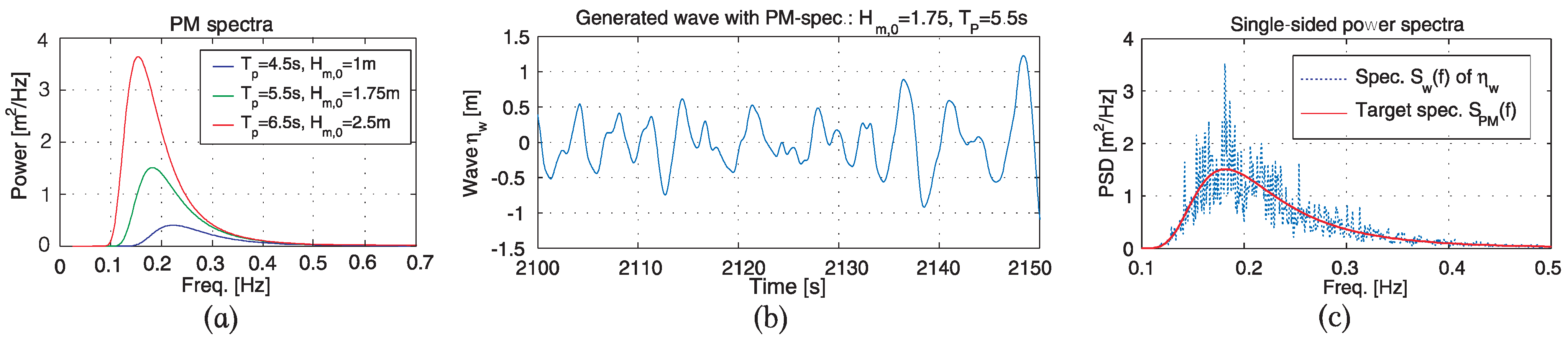
Figure 9a. The figure also shows the three sea states, which are going to be used in the simulation.
Figure 9.
Wave spectra for three sea states and an example of a realization of a wave.
Figure 9.
Wave spectra for three sea states and an example of a realization of a wave.
To perform time simulation, a time realization of a wave is required, complying with the spectrum. Often, the random phase method is used, where the spectrum is converted into a finite number of regular wave components, which are added with a random phase for each component. This simple method has been experienced to be adequate for estimating average power absorption [
25]. However, the method does not reproduce, e.g., wave grouping correctly, according to [
26]. Studies indicate that using the method, the mean length of wave groups is too short [
26]. Thus, the random phase generated waves may not accurately test the PTO’s capability of, e.g., power smoothing and absorption, as this is highly dependent on the degree of wave grouping. Instead, [
26] suggests that by filtering Gaussian white noise, better representation of ocean waves may be achieved, and arbitrarily long series may be generated.
The white noise method is to design a filter according to the PM-spectrum, whereby the filter shapes the power density of the white noise signal to comply with the PM-spectrum. The filers are implemented based on [
11,
27].
If the input process to a filter,
, is white noise, which is defined by having a flat spectrum,
, and the filter,
, is designed according to the PM-spectrum in
Figure 9a,
, then:
where a white noise with variance,
, has been used as input. Thus, by filtering white noise,
, with the filter,
, yields a time series,
, having a spectrum,
, agreeing with the PM spectrum.
The generated wave with this method is shown in
Figure 9b. A spectrum analysis of the generated wave is seen in
Figure 9c, showing fluctuation around the target Pierson-Moskowitz-spectrum. This is desired, as spectrum measurements of real sea waves also have a non-smooth spectrum.
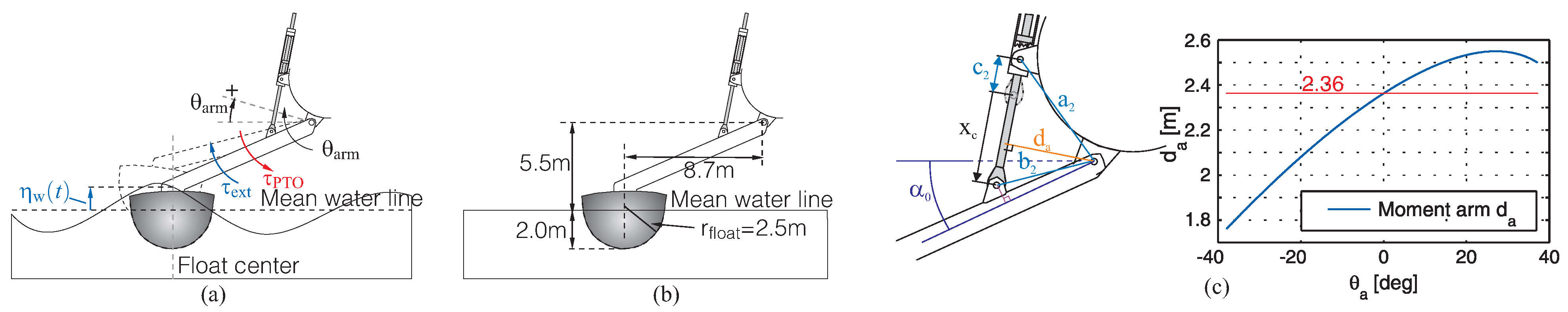
5.1. Absorber Model
The Wavestar absorbers are modeled using linear wave theory, as described in, e.g., [
24], yielding an adequate description in the conditions in which a WEC produces energy. The absorber is illustrated in
Figure 10a, representing a single degree of freedom system expressed by its angular motion,
. The angular position,
, is defined to be zero when the float is horizontal,
i.e., position at calm water. A derivation of the model for single absorber may be found in [
28]. The model here is briefly restated for a single absorber with a diameter of 5 m.
Figure 10.
(a) definition of variables of the Wavestar absorber; (b) some dimensions for the case study; and (c) the moment arm of the cylinder.
Figure 10.
(a) definition of variables of the Wavestar absorber; (b) some dimensions for the case study; and (c) the moment arm of the cylinder.
5.1.1. Single Absorber Model
In linear wave theory, the equation of motion of the absorber is obtained by superimposing the different effects of the wave-absorber interaction:
where the torque,
, is due to Archimedes force; the torque,
, is caused by gravity; the torque,
, is the torque experienced on the absorber from radiating waves;
is the torque applied by the PTO system; and
is the wave excitation torque. The moment of inertia term,
, is the total (mechanical) moment inertia in the
rotation.
By identifying the terms in Equation Equation (
4), the following well-known expression is obtained:
where
is the spring coefficient representing the hydro-static restoring torque;
, which is a linearization of the Archimedes force;
, and gravity,
. In Equation (
4), the radiation term,
, may be expressed as:
where the function,
, is the radiation-force impulse-response function and
is the added inertia at infinite high frequency.
The wave excitation torque,
, is the torque an incoming wave applies to a float held fixed, including the contribution from the float diffracting the wave. A filter for calculating the wave torque based on the wave,
, may be obtained given as an impulse response function,
. The exciting wave torque may then be found by the convolution:
The impulse response, , is non-zero for , rendering the filter non-causal. This mean that the current excitation force depends on the future incident waves. This is partly due to the fact that the waves hit the float before reaching the reference point in the center of the float. Furthermore, the defined wave height is not the direct cause to the wave excitation torque, but is a quantity defined model-wise. Thus, both are caused by some unknown process, and therefore, their relation is not forced to be causal.
To solve this in the simulation, the wave excitation torque is pre-computed before simulation by discrete convolution:
where the impulse response is approximated with a finite impulse response, requiring
samples of future wave knowledge. As the excitation torque is assumed independent of the float motion, but only dependent on the incident wave height, the pre-computation of
is allowed. As the entire wave signal,
, is available beforehand, the non-causality is not a problem.
5.1.2. Multi-Absorber Model
In an array of closely spaced absorbers, such as the Wavestar, the absorbers interact. The absorbers interact in two ways:
The diffraction part may be obtained by placing 20 floats in the given array and, then, identifying the force filter,
, for each float. The resulting diffraction effect experienced by the individual floats will be included in their force filter for calculating the exciting wave torque for each float:
Considering the radiation effect, the equation of motion for each float, before given as Equation (
5), now becomes coupled:
as the matrix,
, containing the radiation impulse responses is non-diagonal:
e.g., the impulse response,
, describes the cross-coupling from the velocity of float number 20 to force on float number 2. Note that
, rendering
symmetric.
With the focus on validating the PTO, the radiation cross terms are neglected in this paper, i.e., for (). Inclusion of the cross terms mostly affects how the absorbers should be controlled to further increase power absorption. Thus, the influence of the float dynamics on the PTO and the cylinder control may be modeled with acceptable accuracy by using a single absorber hydrodynamic model. However, it is still required to have the effect of the floats operating out of phase due to their distributed locations. This is obtained by applying individual force filters, as mentioned previously.
5.1.3. Model Parameters
To obtain the hydro-dynamic model parameters, WAMIT has been applied, which is a program for computing wave loads and motions of structures in waves.
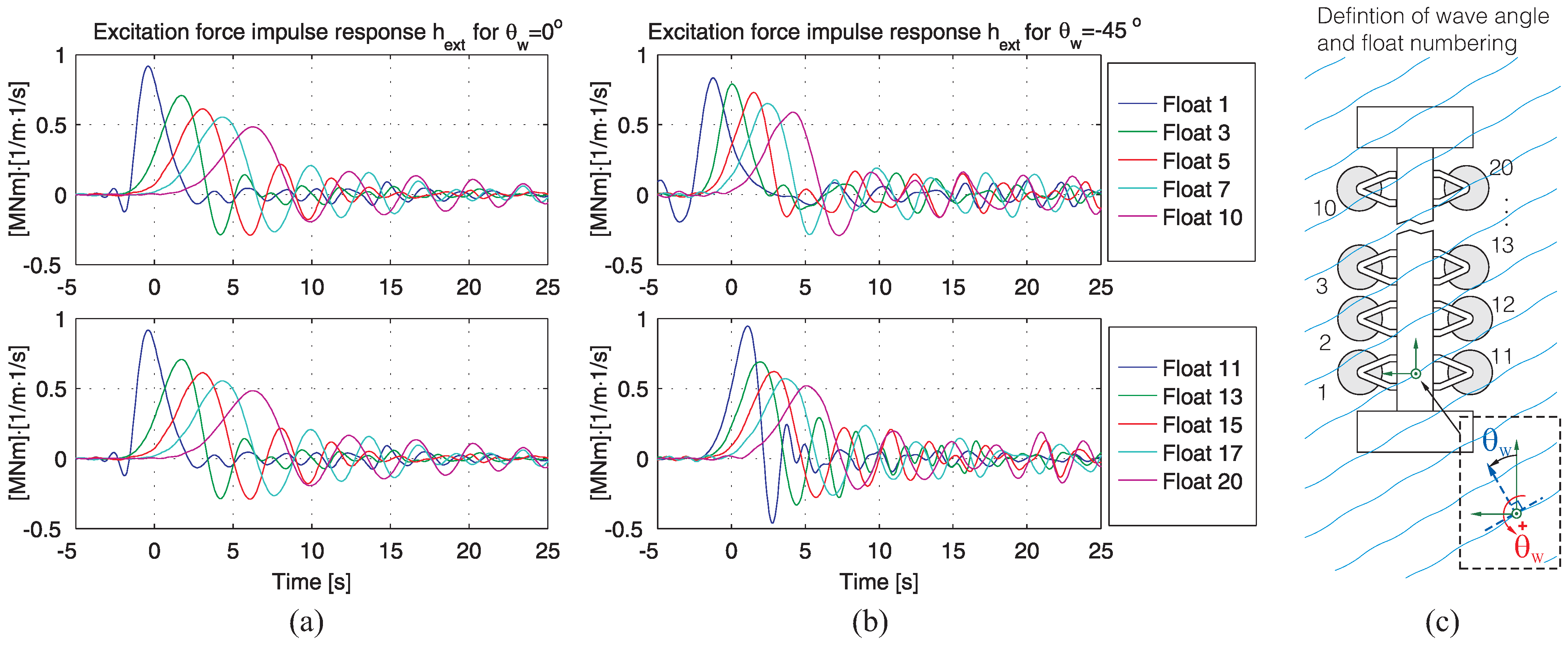
The force excitation filters are shown in
Figure 11 for a wave direction of
and
. The wave “measurement” point is shown in
Figure 11c, along with a definition of float numbering and wave angle,
. The filters show that for
, the wave reaches the floats farthest back (numbers 10 and 20), approximately 7 s later after exciting float number 1. From the plot, it is also seen that there is some amount of shadow effect, as the magnitude of the wave excitation filter reduces for each float. For the
, the input for the float is pair-wise equal, whereas this is not true for the wave angle,
.
Note that the excitation torque is independent of the float movement, i.e., the excitation torque may be calculated “off-line” by the convolution in Equation (7).
From WAMIT, all the impulse-response functions,
, describing the radiation-force are also obtained, including the cross terms (
). However, as theses are neglected, only the single absorber radiation impulse response is used; see
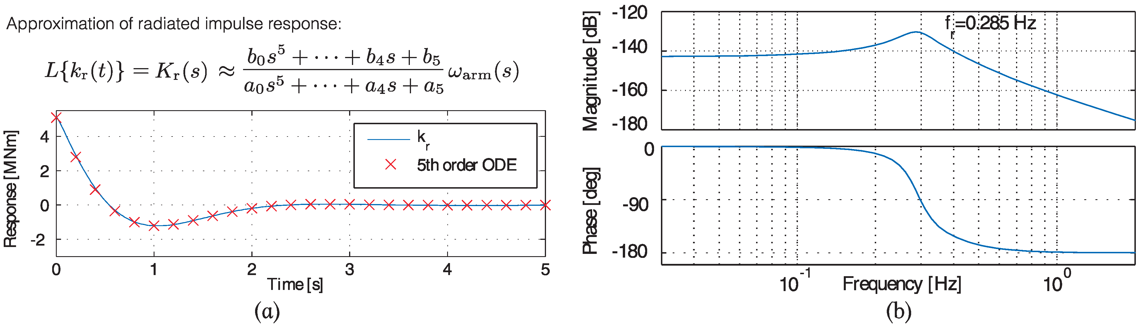
Figure 12a. To avoid performing the convolution term,
, the term is approximated as a system of Ordinary Differential Equations (ODE). This is performed using Prony’s method [
28]. The used fifth order approximation is shown in
Figure 12a.
Figure 11.
The wave excitation force filter impulse responses, , for different floats. (a) is for wave direction, ; (b) is for wave direction, ; and (c), the wave “measurement” point, float numbering and wave angle, , are defined.
Figure 11.
The wave excitation force filter impulse responses, , for different floats. (a) is for wave direction, ; (b) is for wave direction, ; and (c), the wave “measurement” point, float numbering and wave angle, , are defined.
Figure 12.
(a) the impulse response function, , being approximated; and (b) Bode diagram of Equation (12), .
Figure 12.
(a) the impulse response function, , being approximated; and (b) Bode diagram of Equation (12), .
The absorber dynamics may now be written as the following transfer function:
A Bode-diagram of Equation (
12) is given in
Figure 12b with the parameters in
Table 1. The Bode diagram shows that the system has a resonance peak at
, corresponding to a period of 3.51 s. Hence, the Wavestar point absorber will have optimal absorption at a wave period of 3.51 s. At Wavestar C5 production sites, this period corresponds to the sea states with the shortest peak-period, in which a substantial part of the yearly wave energy is concentrated.
Table 1.
Parameter values for the Wavestar C5 absorber.
Table 1.
Parameter values for the Wavestar C5 absorber.
| Parameter | Symbol | Value | Unit |
|---|
| Inertia of arm and float (with ballast water) | | 2.45 | [kgm2] |
| Hydrostatic restoring torque coefficient | | 14.0 | [Nm/rad] |
| Added-inertia for | | 1.32 | [kgm2] |
| Transfer-function coefficients for : |
|
|
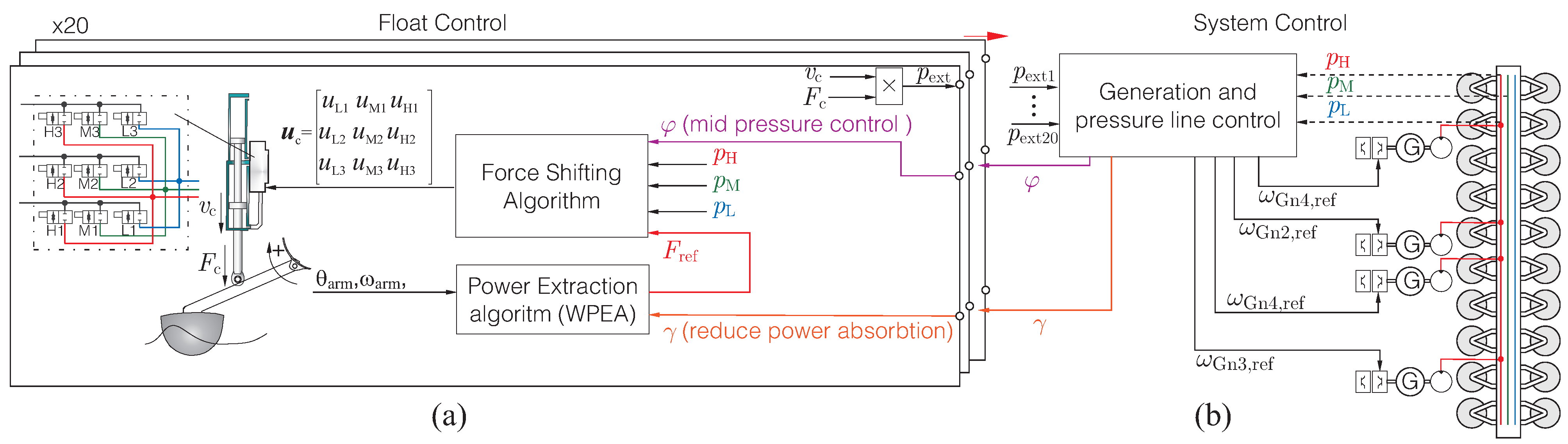
7. PTO Control
The PTO control may be divided into two parts, as shown in
Figure 20. The first part is the float control,
Figure 20a, which controls a DDC-system, compromising between maintaining efficiency and proper power absorption. A Wave Power Extraction Algorithm (WPEA) generates the force reference for optimizing power extraction, while taking into account the PTO efficiency.
The second part is the system control,
Figure 20b, which handles the overall control of pressure lines and power generation,
i.e., the numbers of active generators and their speed references. The system control may also manipulate the float control to put more or less flow into the mid-pressure line (control parameter,
φ) or to reduce the power absorption if the pressure lines are saturated.
7.1. Wave Power Extraction Algorithm
The power extracted by the absorbers from the wave,
, is the product of the applied PTO torque,
, and arm velocity,
(or -
). To maximize the extracted power, the float velocity should be in phase with the exiting wave torque,
,
i.e., the natural frequency of the float and arm should match the incoming wave. However, frequency-wise point absorbers are narrow-banded with an under-damped resonance frequency, as seen in
Figure 12b. Accordingly, point absorbers are prone to operate off-resonance, as the wave period varies wave to wave. On a larger time scale, the average wave period also varies from sea state to sea state, as seen for the wave spectra in
Figure 9.
Figure 20.
(a) float control (20 parallel system), handling the manifold control to track the generated force reference to extract wave power; and (b) system control for controlling generation and pressure lines.
Figure 20.
(a) float control (20 parallel system), handling the manifold control to track the generated force reference to extract wave power; and (b) system control for controlling generation and pressure lines.
To improve the behavior of point absorbers, it is well established that control of the PTO load force may be used, increasing the amount of energy extracted from waves [
4,
5]. Basically, the torque,
, applied to the absorber is controlled as a feedback of the absorber’s motion as:
allowing the PTO to adjust the absorber’s resonance frequency to match the wave frequency. The term,
, is the reactive term and imposes the PTO to implement a virtual spring element, changing the external experienced dynamics of the absorber.
Optimally, the feedback ensures that the velocity of the absorber is always in phase with the wave excitation force and the PTO damping matching the absorbers’ hydrodynamic damping [
4]. However, this requires future knowledge of
for some time,
, rendering the control non-causal. The required wave prediction horizon to remove the non-causal part is approximately the same as the settling time of the system [
4].
A causal and more robust control described for Wavestar in [
28] is to continuously gather statistically information of the current sea state over a window of 100 or more waves. The absorbers narrow frequency response is then widened and adjusted to a fixed resonance frequency, yielding the best average abortion in the current sea state. This may be implemented by having fixed control coefficients in the feedback law Equation (
60). This is a suboptimal approach, but has been applied with good performance results, as reported in [
32].
Optimal adjustment of the absorbers frequency, as the above, requires the PTO to transfer energy to the absorber (assisting its movement) in parts of an oscillation cycle. Thus, the above WPEAs are termed reactive strategies and require a PTO capable of four-quadrant behavior to supply the reactive power. If reactive control is not offered by the PTO, the reactive terms of the control are removed and damping control remains,
i.e., for linear damping control only the coefficient,
, is non-zero in Equation (
60). Linear damping is only optimal when the wave frequency and the absorber’s resonance frequency match by other means.
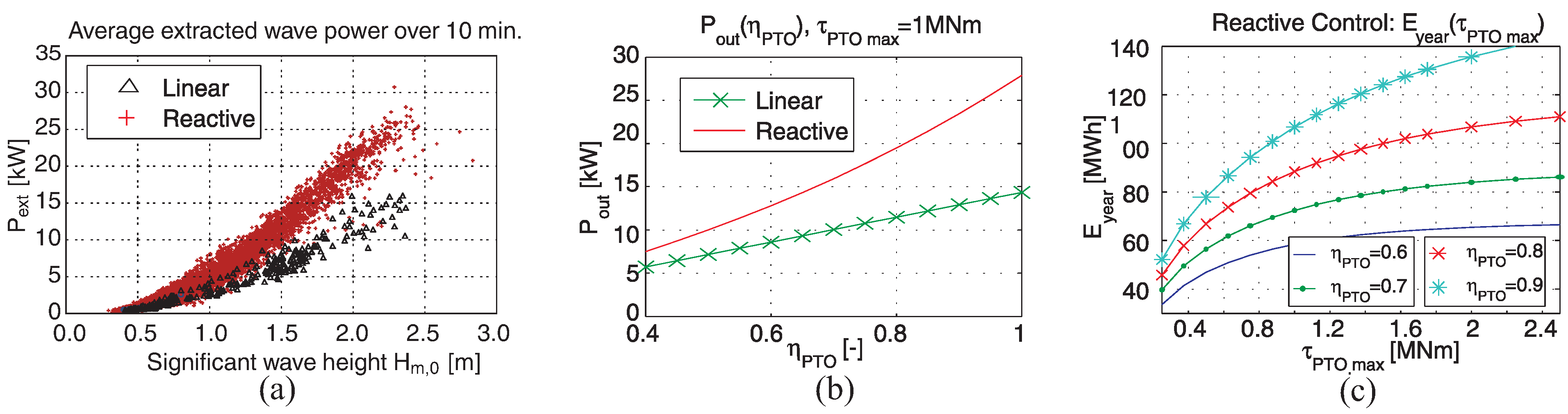
For the Wavestar concept, it has been verified from prototype measurement [
22] that increased production is obtained through reactive control; see
Figure 21a. Each point is an average of extracted power over a 10 min measurement, where both linear damping and reactive control have been tested. The measured average power results are given as a function of significant wave height. Consequently, some of the scatter is due to the different wave periods. The applied control is as in Equation (
60), where the coefficients are fixed for a given sea state. The system continuously gather statistically information of the current sea state over a window of 100 or more waves and, then, choose the coefficients yielding the best average abortion in the current sea state.
Figure 21.
(
a) average extracted power measurements for a single absorber of the prototype in
Figure 5a [
22]. Each point is a 10 min measurement; (
b) comparison of power extraction of linear damping and reaction as a function of efficiency in a sea state with
and
[
11]; and (
c), yearly production of a single absorber at the prototype site [
28] as a function of PTO torque limitation and efficiency [
11].
When optimizing reactive control schemes, it is important to take into account PTO power conversion efficiency, as power is lost in each conversion. Hence, having reactive power oscillating between float and PTO consumes energy. The control in Equation (
60) should always optimize the power output to the grid and not the amount of extracted power.
In [
8,
28], it is shown how the PTO force constraints and conversion efficiency may be included into the control design. The results are a map of control parameters,
and
, as a function of sea state and PTO efficiency. For detailed information on the methods, see [
11].
Figure 22.
(
a) model for reactive control optimization [
8]; and (
b) control parameters for two sea states as a function of PTO power conversion efficiency,
.
Figure 22.
(
a) model for reactive control optimization [
8]; and (
b) control parameters for two sea states as a function of PTO power conversion efficiency,
.
The optimal parameters in [
8,
28] are found by numerically optimizing the output of the simulation model shown in
Figure 22. The model includes the absorber dynamics, and the input to the model is an irregular sea wave,
. The PTO is characterized by a force limitation and an efficiency. The PTO power output may then be formulated as a function of the extracted power,
:
The optimal control parameters for Equation (
60) is then found as the arguments maximizing the energy output of the PTO:
The optimal values of
and
for two sea states are shown in
Figure 22b. These results are from [
11]. Here, it is seen as expected, that when the PTO conversion efficiency,
, is reduced, the reactive part (
) reduces and the resistive part increases. To further justify the reactive control, a comparison of reactive control and linear damping is shown in
Figure 21b [
11]. It shows that despite having a power conversion efficiency of, e.g., 70%, 50%, more power is produced to the grid compared to linear damping.
The torque requirement of the PTO is chosen to be
, which is a compromise made according to
Figure 21c, as the PTO efficiency is expected to be about 70%. In
Figure 21c, the yearly production for a single absorber has been computed in [
11] by calculating the average power output for all sea states and, then, assuming a yearly wave distribution.
To summarize, given the sea state and PTO information,
, the force reference to the cylinder is calculated as:
where
is the moment arm and
γ is a coefficient, which the system control may use to reduce the power absorption if the pressure lines are saturated. To reduce power absorption, a method could also have been to reduce the efficiency input to the WPEA algorithm, forcing the WPEA to move towards linear damping, thereby reducing power absorption and system stress.
The actual PTO efficiency is not independent of the WPEA defined in Equation (
63). Adjusting the reactive power may either improve or reduce component performances, depending on whether the increased power level brings the components closer to their rated/optimum power level. To this account, an initial efficiency estimate is given to find the WPEA, and through simulation of the PTO, a new efficiency is obtained, which is used to update the WPEA. A number of iterations have been performed to find the proper settings. This is also discussed in [
8] for the Wavestar converter.
The force control is going to be implemented discretely,
i.e., the continuous reference generated by Equation (
63) is subjected to a quantification. To investigate the influence, comparison of a continuous control and a discrete control has been performed.
The continuous control is simulated as in
Figure 22a, with the optimum parameters, a PTO efficiency of 70% and a maximum torque of ±1 MNm. The simulation of the discrete version is implemented likewise with the same WPEA parameters, but the PTO torque is quantified before being applied to the float. The available torque values besides zero are set to 9 evenly spaced values between
. Moreover, a limit is set on the shift rate, limiting the force to shift at maximum one time per 300 ms. Thus, after a shift has occurred, the force value is locked for 300 ms, whereafter the quantification process may choose the force closest to the continuous reference. This avoids the risk of jittering and PWM (Pulse Width Modulated)-like behavior and keeps the number of shifts at a reasonable level. The results are seen in
Figure 23, showing the two power matrices of average produced power. As seen, the difference is relatively low despite the relatively rough quantization. Thus, the force approximation of the DCC having 27 force values will be adequate.
Figure 23.
Power matrices of average produced power in [kW]. The matrices are shown for a continuous torque control and a discrete control with force values.
Figure 23.
Power matrices of average produced power in [kW]. The matrices are shown for a continuous torque control and a discrete control with force values.
The reason for the low impact of the discrete variation is that the 35 tons of the float and arm system serve as an effective low pass filter, having a break frequency around 0.28 Hz, c.f. the earlier calculated natural period of 3.5 s. Thus, from a load control point of view, implementation of extra dampers/low pass filters is not required.
Another aspect is the compliance of the mechanical structure when performing the rapid load force changes; however, these issues are not treated in this paper. One aspect to notice, though, is that the force steps are relatively small, e.g., a single step from zero to maximum is never performed.
7.2. DDC Control—Force Shifting Algorithm (FSA)
The purpose of the Force Shifting Algorithm (FSA), controlling the DDC, is to choose the appropriate force level to approximate the reference,
, generated by the WPEA. However, always shifting to the force closest to the continuous reference,
, may not energy-wise be optimal, as some force-shifts are more energy-expensive than others, due to the compression loss,
. The minimum compression loss of a volume when shifting
, independent of the pipe line dynamics [
33], is given as [
16]:
This loss is illustrated in
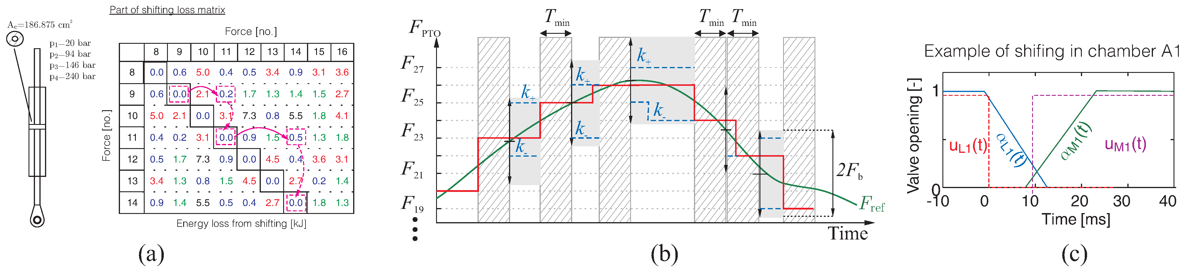
Figure 24a for a system consisting of four system pressures and a symmetric cylinder. The figure shows the compression loss in [kJ] from shifting between forces. The forces are sorted according to size. As illustrated, if the current force is force number 9 and an increase in force is desired, it is cheaper to shift to force number 11 instead of 10. Likewise, from number 11, it is cheaper to shift to number 14 and skip 12 and 13. Thus, to avoid doing very expensive force shifts, a more suitable strategy is to calculate the energy expense of possible force-shifts and make a compromise between tracking and energy-cost. This is the basis of the FSAstrategy developed in [
15] and which is also used in this study. Note that the loss matrix changes with pressure and cylinder position.
Figure 24.
(a) illustration of the shifting loses due to compression; (b) illustration of the force shifting algorithm; and (c) the opening and closing procedure of the valves during shifting.
Figure 24.
(a) illustration of the shifting loses due to compression; (b) illustration of the force shifting algorithm; and (c) the opening and closing procedure of the valves during shifting.
The shifting loss from shifting from force
x to
y is found summing the losses Equation (
64) for pressure changes in the individual volumes:
Note that the pressures, , may be equal, as the pressure is not necessarily shifted in all chambers.
To allow compromising between force tracking and performing less expensive force shifts, a maximum allowed tracking error, , is defined, meaning that must stay within a band of about . However, within the band, the FSA may choose the force steps with the lowest shift cost. A fixed time limit, , on how frequently shifting is allowed is also added to reduce tracking cost.
The FSA algorithm is illustrated in
Figure 24b. The values,
and
, are the numbers of the forces, which are the cheapest to shift to within the band,
. As seen, these are continuously updated. When the force reference comes closer to one of the forces,
or
, a shift is performed, and a new lock down period of
is initiated.
Based on the optimization procedure in [
15], it has been found that
and
for optimizing the power output of the Wavestar C5.
Thus, when a force shift is initiated, the control sends out a matrix,
, of control values for the nine on/off valves, corresponding to the desired pressure configuration. Regarding valve timing, it was found in [
16] that a small amount of overlap between opening and closing of the valves for a single volume was desirable; thus, a 3 ms overlap is used. As the valves have 12 ms opening and closing time, the signal to the opening valve is delayed 9 ms. This is illustrated in
Figure 24c.
To help in controlling the pressure in the mid-pressure line, the FSA continuously identifies the force combinations that would currently supply or consume flow from the mid-pressure line. For these configurations, an “artificial” energy loss,
φ, may be added in Equation (
65) by the system control to either penalize supplying or consuming flow from the mid-pressure line.
7.3. System Control
The purpose of the system control is to:
Avoid the high pressure accumulator storage from depletion or saturation;
Keep the mid-pressure line floating between high and low pressure;
Ensure as steady a power production as possible, while satisfying 1 and 2;
Choose the proper number of generators for a given sea state;
Reduce power absorption when full load capacity is reached.
To maintain a stable power production, the generators are set to initially produce the expected average power, , in the current sea state. An initial guess is given based on the current sea state when starting production, whereafter a moving average is used based on the absorbed power over a window of 5 min. The number of active generators, , is then chosen, such that generation capacity is roughly plus 30%. All active generators are operated at the same speed .
To avoid the high pressure accumulator storage from depleting or saturating, the power generation is increased or decreased based on the pressure in the accumulators. This is performed through the coefficient,
ψ. The speed reference is then given as
:
where
is the total active motor displacement in [m
3/rad]. As
is the absorber power, the efficiency from cylinder to power out of the generator,
, is required to calculate the average generator power. The maximum allowed speed is set according to 180 kW per generator, which is 15% overload. The lowest speed is set to 400 RPM.
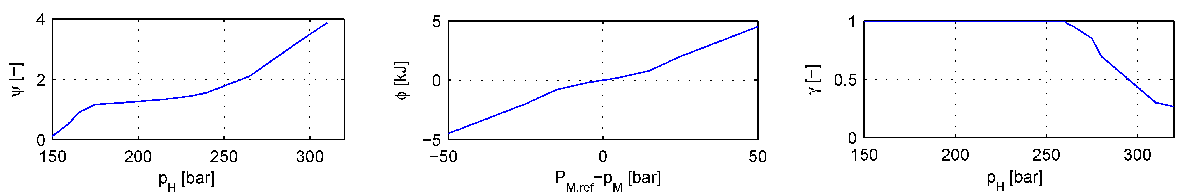
The high pressures are set to be between 150 bar and 300 bar; thus, the map in
Figure 25 for
ψ is used. Finally, if pressure is still reaching 300 bar, the value,
γ, is manipulated, such that the float reduces power absorption; see
Figure 25. This is similar to turbines pitching out of the wind when rated production is reached.
Figure 25.
Maps for the different system control parameters, ψ, φ and γ.
Figure 25.
Maps for the different system control parameters, ψ, φ and γ.
The mid-pressure is to be floating between high and low pressure for optimizing the DDC efficiency. Hence, the “reference”,
, for the mid-pressure line is:
Based on this, the penalty value,
φ, is set according to
Figure 25.
9. Conclusions
The paper has demonstrated a PTO-system for the Wavestar WEC capable of solving the following challenges:
Handling peak power input, which is a factor of 12 higher than mean power, while maintaining component efficiency—the DDC maintains above 90% in these conditions, and the remaining components are above 94% in efficiency, each;
Full controllability of load force on absorbers and four quadrant mode—the DDC offers 27 force steps and four quadrant mode;
Incorporating a short-term storage for supplying reactive power—reactive power is only processed by DDCs and accumulators;
Incorporating an efficient energy storage for power smoothing—generators are operated independent of the wave absorption; energy storage for operating generators at 1500 RPM for one minute;
Maintaining PTO efficiency in small waves when operating at 15% of full load capacity—total efficiency maintained above 70% in all sea states;
Being able to reduce power absorption when full load capacity is reached—the DDCs reduce absorption when the WEC reaches full load;
Being scalable to future multi-MW systems.
Based on rigorously modeling the system from wave-to-wire, the overall efficiency of the PTO was found to beyond 70% in all sea conditions, while providing excellent power absorption.
The utilized power absorption algorithms (WPEA) were based on reactive control methods, tuning the resonance of the system. The algorithms were tuned to take into account the efficiency of the PTO to maximize electrical power production.
The WPEA determined load force reference was applied using the specially developed DDC-modules mounted on each float, consisting of discrete controlled multi-chambered cylinders. The DDC modules directly convert and store the absorbed wave power as high pressure energy in the accumulators with a loss less than 10%.
The implemented PTO system had an extra intermediate pressure line for improved efficiency of the DCC. It was shown that by overall system control, the net flow to the intermediate line could be kept at zero; hence, extra pumps and motors for supporting this line are not required. The simulations verified that when reaching full load capacity, the system would reduce the power absorption using the DDCs, such that full load is sustained, but no extra energy has to be dissipated internally in the system.
Regarding scalability, the DDC-modules are fully scalable to be increased to larger systems. Currently, commercial valves with the required transient opening and closing times (≤15 ms) are available with only 2% loss at and with a peak power level of more than 4 MW. This is more than required for, e.g., a 6 MW Wavestar system with 20 floats. Furthermore, valves may be easily used in parallel, thereby also increasing redundancy. Regarding hydraulic motors, commercial 1000 cc high speed motors are available, producing 750 kW at 300 bar and 1500 RPM. Within the wind turbine industry, hydraulic transmission are also being investigated, leading to development of fast multi-MW motors with high efficiency; see, e.g., Digital Displacement® technology. These variable displacement also shows high part load efficiency, leading to the option of operating at a fixed generator speed of the 1500 RPM, thereby potentially removing the power converters.
The size of the storage may be increased as desired. The storage size is a cost optimization problem between power smoothness and accumulator cost. Increasing the storage does not reduce the overall efficiency, as the round-trip efficiency of accumulators is around 97%. Instead, increasing storage may increase efficiency and durability, as it narrows/stabilizes the operating region of the remaining PTO components, thereby making them operate near their optimum point at a constant load.
Looking at potential improvements, the control of the DDC-modules presented in this paper is a simplified version, not taking into account, e.g., cylinder velocity and simultaneous shifting of multiple-chambers. The system control is also a very simplified version, which does not use the energy storage at full potential to stabilize and increase energy production. Additionally, further optimization on the pressure line network may be performed, reducing pipe losses and improving transient behavior. Improved hydraulic motor-efficiencies are also obtainable with commercial available components (96% efficiency) and coming digital displacement motors. Using the rigid-body assumption, it was through simulation verified that the discrete force control yielded approximately the same energy extraction performance as a continuous control. However, regarding compliance of the mechanical system, the presented work did not cover this issue. For example, when using the DDC, there is a risk of exciting the structural eigen-frequencies. Thus, when applying the described DDC, a detailed dynamical mapping of the mechanical system should be performed as a part of the DDC design.
With the potential improvements, the PTO concept has been assessed to be able to reach about 80% efficiency from mechanical input to electrical output.


