An Analysis of Variable-Speed Wind Turbine Power-Control Methods with Fluctuating Wind Speed

Abstract

Variable-speed wind turbines (VSWTs) typically use a maximum power-point tracking (MPPT) method to optimize wind-energy acquisition. MPPT can be implemented by regulating the rotor speed or by adjusting the active power. The former, termed speed-control mode (SCM), employs a speed controller to regulate the rotor, while the latter, termed power-control mode (PCM), uses an active power controller to optimize the power. They are fundamentally equivalent; however, since they use a different controller at the outer control loop of the machine-side converter (MSC) controller, the time dependence of the control system differs depending on whether SCM or PCM is used. We have compared and analyzed the power quality and the power coefficient when these two different control modes were used in fluctuating wind speeds through computer simulations. The contrast between the two methods was larger when the wind-speed fluctuations were greater. Furthermore, we found that SCM was preferable to PCM in terms of the power coefficient, but PCM was superior in terms of power quality and system stability.

1. Introduction

Renewable energy sources have attracted growing research interest in recent years, particularly wind power, whose commercial installations in about 80 countries at the end of 2011 totaled about 240 GW [1]. Its average cumulative growth rates over 15 years amount to about 28%. In the early 1990s, fixed-speed wind turbines (FSWTs) were widely installed; however, FSWTs have drawbacks, including uncontrollable reactive power, excessive mechanical stress, and limited power-quality control. Recently, the variable-speed wind turbine (VSWT), which uses a power converter and hence is more controllable than a FSWT, has become the dominant type of wind turbine due to the increasingly more strict technical requirements of the grid operation codes [2]. There are three different types of wind turbine (WT) among VSWTs [3]. One of them uses a full-scale converter, another one uses a partial-scale converter, which is usually a doubly fed induction generator (DFIG), and the third one does not use power converter. VSWTs typically employ a maximum power-point tracking (MPPT) method to acquire the maximum amount of energy from the wind. The MPPT adjusts the angular velocity of the rotor to an optimum speed, corresponding to the wind speed, for maximizing the active power output, while the wind speed fluctuates. However, the active power fluctuates as the wind speed varies, which may lead to power quality and the power system stability issues.

In previous years, when the penetration level of wind power was low, the impact of these fluctuations in the output from WTs on the power system stability was minimal and, accordingly, regulations on WTs were unnecessary. However, the increasing wind-power penetration levels in modern power systems has led to specific technical requirements for the connection of large wind farms, usually as a part of the grid codes issued by the transmission system operators [4]. Grid codes for WTs include requirements for active and reactive power control, frequency and voltage deviation under normal operation, and behavior during grid disturbances [3,4,5]. Among these requirements, active power control is the most significant issue for power quality and system stability since the others can be easily met by controlling the reactive power output of the grid-side converter (GSC) of a VSWT, whereas the active power output is more strongly dependent on the wind speed.

For this reason, much research has been carried out into controlling the active power of VSWTs to smooth wind-power output [6,7,8] or to support frequency control [9,10,11]. A simple coordinated control method of a direct current (DC)-link voltage and pitch angle of a VSWT with a permanent magnet synchronous generator (PMSG) to smooth the output power is described in reference. [6]. In addition, a constant power-control scheme for a wind farm equipped with DFIG wind turbines with a super capacitor energy-storage system has been proposed [7]. Control strategies for optimal use of a battery energy-storage system integrated with a large wind farm have also been proposed [8]. Reference [9] describes a method to allow VSWTs to emulate inertia and support primary frequency control using the kinetic energy stored in the rotating mass of the turbine blades. This has been expanded to achieve a frequency response capability of a full converter VSWT with a PMSG [10], where a control scheme is used that improves the frequency control, illustrating the importance of the initial active power output of the VSWT generator. Reference [11] describes a strategy to provide frequency regulation for DFIGs by using pitch angle and modified linear slope control.

The studies described above represent attempts to mitigate wind-power fluctuations or support frequency control by adjusting the active power output of the WT. References [6,9] used regulation of the rotor speed at the outer control loop of the machine-side converter (MSC) to control the active power of the WT, while the other studies used direct control of the active WT power. However, all of these researchers have overlooked the differences between speed-control mode (SCM) and power-control mode (PCM). Therefore, to identify the differences between the two methods and prevent indiscriminate use of them, we have compared and analyzed these two control modes from the point of view of power quality and the power coefficient. The differences between the two methods during fluctuating wind speeds are illustrated by simulated data. Since the VSWT model used in this paper is a full-converter WT, the simulated data should be referred to the same type of WT for its application.

2. Wind Energy Conversion System

Figure 1 shows a schematic diagram of a wind-power generation system. It consists of a gearbox, a PMSG, a MSC, a DC-link capacitor, a GSC, and a filter. To implement MPPT, the rotational speed of the PMSG is controlled by the MSC using either SCM or PCM. The output power is delivered to the power system, which is modeled as an infinite bus in this paper, through the MSC and GSC. The GSC controller keeps the DC-link voltage constant and controls the reactive power output. If the gearbox is considered as non-ideal, factors such as backlash, mesh stiffness, and meshing error are reflected to the gearbox model [12]. This makes the problem complicated, so for convenience, the gearbox is assumed to be ideal since the analysis of this study is focused on the performance of the electrical parts of the system.

Figure 1. Schematic diagram showing an overview of the wind energy conversion system.

Figure 1. Schematic diagram showing an overview of the wind energy conversion system.

2.1. Wind Turbine Model

The power that can be extracted from the wind, $P_w$, is given by the following relationships:

$$P_w=\frac{1}{2}\rho \pi r^2{v}_w^3{C}_p\left(\lambda ,\beta \right)$$

(1)

$$\lambda =\frac{{\omega }_{t}r}{v_w}$$

(2)

where $\rho$ is the density of the air; $r$ is the radius of the wind turbine; $v_w$ is the wind speed; $C_p$ is the wind turbine power coefficient; $\lambda$ is the tip speed ratio; ${\omega }_t$ is the angular velocity of the wind turbine rotor; and $\beta$ is the pitch angle; $C_p$ is given by [3]:

$$C_p=0.73\left(\frac{151}{{\lambda }_i}-0.58\beta -0.002{\beta }^{2.14}-13.2\right)e^{-18.4/{\lambda }_i}$$

(3)

$${\lambda }_i={\left[\left(\frac{1}{\lambda -0.02\beta }\right)-\left(\frac{-0.003}{{\beta }^3+1}\right)\right]}^{-1}$$

(4)

Since the analysis will be carried out using the MPPT configuration, the pitch angle $\mathsf{\beta }=0°$. Then, the maximum power coefficient $C_{p,max}$ = 0.4412 at the optimum tip speed ratio ${\lambda }_{opt}$ = 7.206, as shown in Figure 2.

Figure 2. Relationship between the power coefficient $C_p$ and the tip speed ratio $\lambda$.

Figure 2. Relationship between the power coefficient $C_p$ and the tip speed ratio $\lambda$.

Using Equations (1) and (2), the maximum power from the wind can be calculated from:

$$P_{w,max}=\frac{1}{2}\rho \pi r^2{C}_{p,max}{\left(\frac{{\omega }_{t,opt}r}{{\lambda }_{opt}}\right)}^3=K_{opt}{\omega }_{t,opt}^3$$

(5)

where:

$$K_{opt}=\frac{1}{2}\rho \pi r^2{C}_{p,max}{\left(\frac{r}{{\lambda }_{opt}}\right)}^3$$

(6)

$${\omega }_{t,opt}=\frac{{\lambda }_{opt}{v}_w}{r}$$

(7)

The optimum angular velocity of the generator rotor ${\omega }_{m,opt}$ and the optimum electrical angular velocity of the generator rotor ${\omega }_{e,opt}$ can be calculated from:

$${\omega }_{m,opt}=N_{gr}{\omega }_{t,opt}$$

(8)

$${\omega }_{e,opt}=N_{pp}{\omega }_{m,opt}$$

(9)

where $N_{gr}$ is the gear ratio and $N_{pp}$ is the number of pole pairs in the PMSG.

2.2. PMSG Model

The voltage and torque relationships for the PMSG in the $dq$ reference frames are given by the following equations:

$$v_{md}=R_s{i}_{md}+L_d\frac{d{i}_{md}}{dt}-{\omega }_e{L}_q{i}_{mq}$$

(10)

$$v_{mq}=R_s{i}_{mq}+L_q\frac{d{i}_{mq}}{dt}+{\omega }_e{L}_d{i}_{md}+{\omega }_e{\lambda }_{pm}$$

(11)

$$T_e=\frac{3}{2}{N}_{pp}\left\{{\lambda }_{pm}{i}_{mq}+\left(L_d-L_q\right)i_{md}{i}_{mq}\right\}$$

(12)

where $v_{md}$ and $v_{mq}$ are the stator $dq$-axis voltages; $i_{md}$ and $i_{mq}$ are the stator $dq$-axis currents; $R_s$ is the stator resistance; $L_d$ and $L_q$ are the $dq$-axis inductances; ${\omega }_e$ is the electrical angular velocity of the generator rotor; ${\lambda }_{pm}$ is the permanent magnetic flux; and $T_e$ is the electromagnetic torque. For simplicity, we assume that the damping of the turbine and the generator can be neglected as many other literatures did [11,13,14,15,16]. Then, the rotational speed of the generator rotor and wind turbine driving torque can be expressed as:

$$T_m-T_e=J_{eq}\frac{d{\omega }_m}{dt}$$

(13)

where $T_m$ is the mechanical torque of the generator; $J_{eq}$ is the total equivalent inertia referred to the generator; and ${\omega }_m$ is the mechanical angular velocity of the generator rotor.

2.3. Machine-Side Converter Control

From Equations (10) and (11), the inner control loop of the MSC controller can be implemented as shown in Figure 3. The signals $i_{md}$ and $i_{mq}$ are compared to their reference signals $i_{md}^{*}$ and $i_{mq}^{*}$, and the error signals form inputs to the proportional-integral (PI) controllers.

Figure 3. Circuit diagram of the MSC inner control loop.

Figure 3. Circuit diagram of the MSC inner control loop.

To decouple the d- and q-axes, the ${\omega }_e{L}_q{i}_{mq}$ term is subtracted from output signal of the d-axis current controller, and ${\omega }_e{L}_d{i}_{md}$ and ${\lambda }_{pm}{\omega }_e$ terms are added to output signal of the q-axis current controller. The final control voltages $v_{md}^{*}$ and $v_{mq}^{*}$ are proportional to the converter output voltages $v_{md}$ and $v_{mq}$; therefore, the control configuration regulates $i_{md}$ and $i_{mq}$ using $v_{md}^{*}$ and $v_{mq}^{*}$, respectively.

The reference signals $i_{md}^{*}$ and $i_{mq}^{*}$ are determined by the outer control loop of the MSC controller. Since $T_e$ is a nonlinear function of the machine currents, an approach that avoids nonlinearities is to impose $i_{md}^{*}=0$ [17]. This reduces Equation (12) to:

$$T_e=\frac{3}{2}{N}_{pp}{\lambda }_{pm}{i}_{mq}$$

(14)

Equation (14) shows that $T_e$ can be controlled only by $i_{mq}$, since $N_{pp}$ and ${\lambda }_{pm}$ are constant. Two different methods of providing $i_{mq}^{*}$ are considered in this paper. One of them is SCM, which adjusts ${\omega }_e$, and the other is PCM, which adjusts $P_{out}$, as shown in Figure 4. In the MPPT method, the reference signals for PCM and SCM are $P_{out}^{*}=K_{opt}{\omega }_t^3$ and ${\omega }_e^{*}={\omega }_{e,opt}$, respectively, which follows from Equations (5) and (9). A comparison of these two modes is described in more detail in Section 3, and forms the main theme of this paper.

Figure 4. Two different modes of the MSC outer control loop.

Figure 4. Two different modes of the MSC outer control loop.

2.4. Grid-Side Converter Control

The voltage balance across the filter, shown in Figure 1, is given by the following equations:

$$v_{gd}=R_f{i}_{gd}+L_f\frac{d{i}_{gd}}{dt}-{\omega }_s{L}_f{i}_{gq}+v_{sd}$$

(15)

$$v_{gq}=R_f{i}_{gq}+L_f\frac{d{i}_{gq}}{dt}+{\omega }_s{L}_f{i}_{gd}+v_{sq}$$

(16)

where $v_{gd}$ and $v_{gq}$ are the GSC output dq-axis voltages; $i_{gd}$ and $i_{gq}$ are the GSC output dq-axis currents; $v_{sd}$ and $v_{sq}$ are the point of common coupling (PCC) dq-axis voltages; $R_f$ and $L_f$ are the resistance and inductance of the grid filter, respectively; and ${\omega }_s$ is the angular frequency of the PCC voltage. Based on Equations (15) and (16), the control scheme of the GSC is shown in Figure 5.

The inner control loop of the GSC is operated in similar way to that of the MSC. The outer control loop of the GSC provides $i_{gd}^{*}$ and $i_{gq}^{*}$, which are the reference signals for $i_{gd}$ and $i_{gq}$, respectively. In the PCC voltage-oriented frame, we assume that the loss on the filter is negligible, and that the active and reactive power values transferred from the GSC to the grid are proportional to $i_{gd}$ and $i_{gq}$, respectively, as shown by the following equations:

$$P_{out}=\frac{3}{2}\left(v_{gd}{i}_{gd}+v_{gq}{i}_{gq}\right)=\frac{3}{2}{v}_{gd}{i}_{gd}$$

(17)

$$Q_{out}=\frac{3}{2}\left(v_{gq}{i}_{gd}-v_{gd}{i}_{gq}\right)=-\frac{3}{2}{v}_{gd}{i}_{gq}.$$

(18)

Figure 5. GSC control structure.

Figure 5. GSC control structure.

Hence, $Q_{out}$ is controlled by varying $i_{gq}$, as shown in Figure 5. $Q_{out}^{*}$ = 0 is imposed to maintain the unity power factor at the PCC. We define the reference signal $i_{gd}^{*}$ by regulating the DC-link voltage $V_{dc}$ instead of $P_{out}$, since the active power transferred from the PMSG to the grid is determined by adjusting the MSC. This is illustrated in Figure 6, and is expressed by the following relationships:

$$P_{MSC}=P_{GSC}+P_C$$

(19)

$$P_C=V_{dc}{I}_{dc}=V_{dc}C\frac{d{V}_{dc}}{dt}$$

(20)

where $P_{MSC}$ is the active power transferred from the MSC to the DC-link; $P_{GSC}$ is the active power transferred from the DC-link to the GSC; $P_C$ and $I_{dc}$ are the active power and the current through the DC-link capacitor, respectively; and $C$ is the capacitance of the DC-link capacitor. From Equations (19) and (20), $P_{GSC}$ can be regulated by adjusting $V_{dc}$, which is kept constant in this study. Consequently, assuming that all the line and converter losses can be ignored, $P_{PMSG}$ the active power transferred from the PMSG to the MSC, $P_{PMSG}$, which is adjusted by the MSC controller, can be made equal to $P_{out}$.

Figure 6. DC-link power flow.

Figure 6. DC-link power flow.

3. Case Study

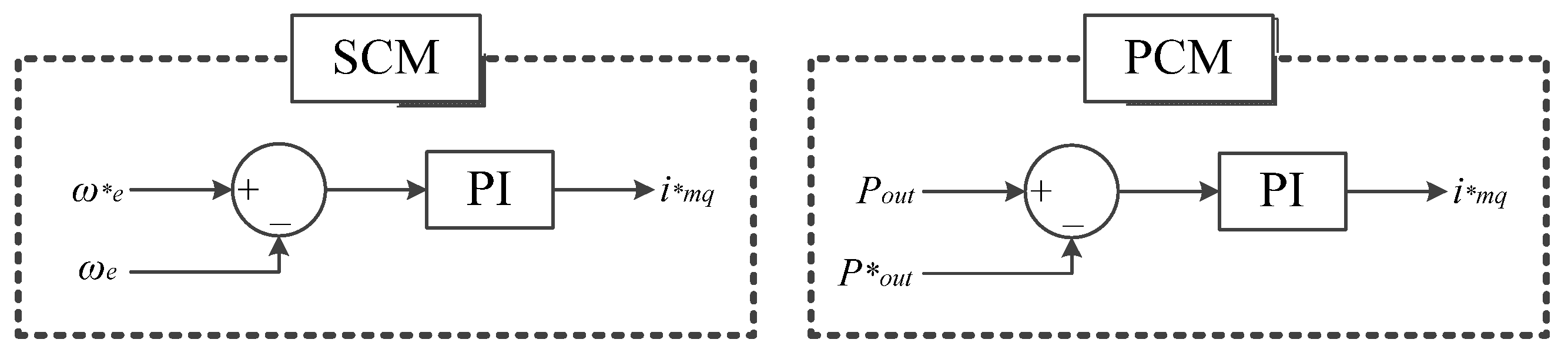
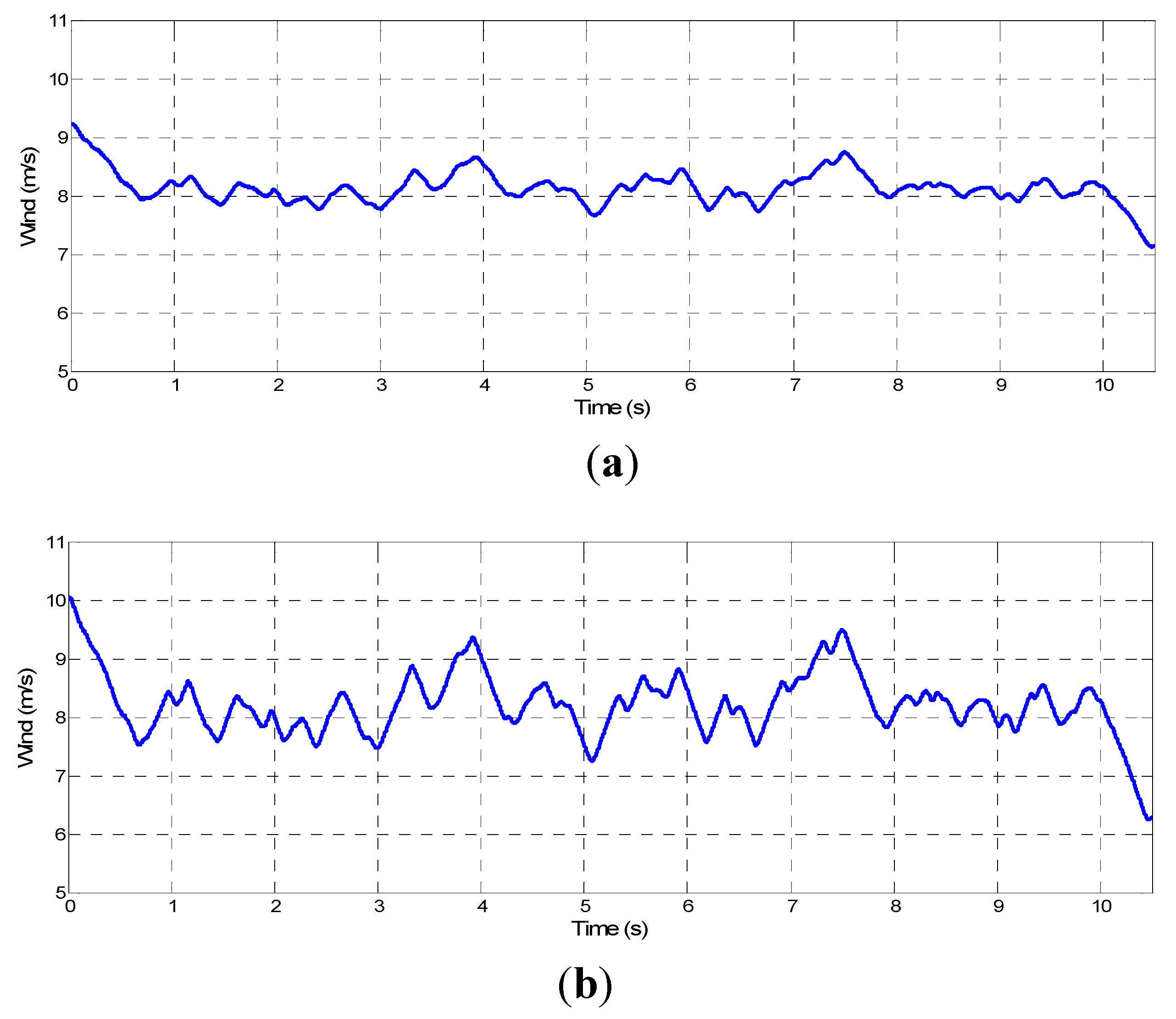
An analysis of the differences between SCM and PCM is described in this section. MPPT was used, since it is the most common method to control VSWTs. In theory, SCM and PCM are equivalent because they both control the active power. However, due to the differences in the time delays of the control loop, differences exist between applying SCM or PCM at the outer control loop of the MSC. These differences become greater as the wind-speed fluctuations become more severe. To illustrate this, two cases were investigated for both SCM and PCM. For each case, we used the same mean wind speed. However, the rate of change and the amount of change of the wind speed were varied, as shown in Figure 7. Since it can be expected and obvious that there will be no differences between SCM and PCM when the wind speed is constant, a case of constant wind speed is disregarded in the case study.

Figure 7. Time dependence of the wind speed for (a) case 1 and (b) case 2.

Figure 7. Time dependence of the wind speed for (a) case 1 and (b) case 2.

3.1. Simulation Results

Simulations were developed using MATLAB/SimPowerSystems to investigate these two cases using both SCM and PCM. The characteristics of the modeled wind turbine are summarized in Table 1.

Table 1. Characteristics of the wind turbine used in the simulations.

Parameters	Value	Unit
Rated power	7.35	MW
Rotor radius	83.5	m
Nominal wind turbine rotor speed	0.936	rad/s
Gearbox ratio	30	-
Number of pole pairs	9	-

Table 1. Characteristics of the wind turbine used in the simulations.

Parameters	Value	Unit
Rated power	7.35	MW
Rotor radius	83.5	m
Nominal wind turbine rotor speed	0.936	rad/s
Gearbox ratio	30	-
Number of pole pairs	9	-

Since voltage and frequency at the PCC are affected by characteristics of the transformer and the infinite bus, and hence the simulation results which contain performances of the power quality are related to them, it is useful to provide characteristics of the transformer and the infinite bus. They are shown in Table 2 and Table 3, respectively.

Table 2. Characteristics of the transformer used in the simulations.

Parameters	Value	Unit
Nominal power	7.35	MVA
Nominal primary/secondary voltage	3.3/22.9	kV
Primary and secondary resistance/inductance	0.002/0.08	p.u.

Table 2. Characteristics of the transformer used in the simulations.

Parameters	Value	Unit
Nominal power	7.35	MVA
Nominal primary/secondary voltage	3.3/22.9	kV
Primary and secondary resistance/inductance	0.002/0.08	p.u.

Table 3. Characteristics of the infinite bus in the simulations.

Parameters	Value	Unit
3-phase short-circuit level at base voltage	100	MVA
Base voltage	22.9	kV
X/R ratio	7	-

Table 3. Characteristics of the infinite bus in the simulations.

Parameters	Value	Unit
3-phase short-circuit level at base voltage	100	MVA
Base voltage	22.9	kV
X/R ratio	7	-

To determine whether the electrical rotor speed properly tracks the optimal electrical rotor speed, the rotor speeds for SCM and PCM were measured. The power coefficient was measured to compare the efficiencies of SCM and PCM. To analyze the relative power quality between SCM and PCM, the active power output, frequency, and root mean square (RMS) voltage were measured. The subscripts SCM and PCM are used to denote which mode was used for controlling the active power of the wind turbine.

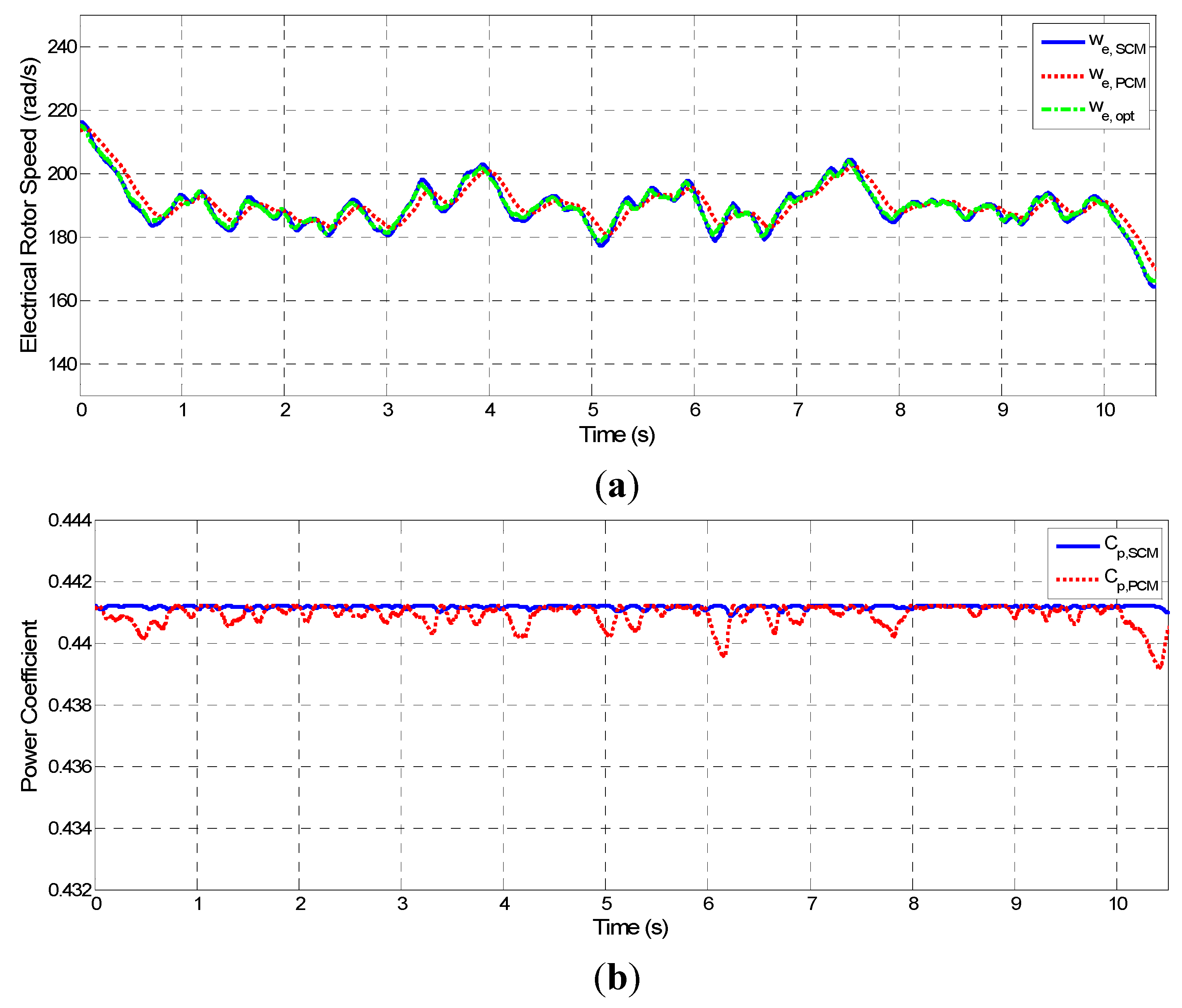
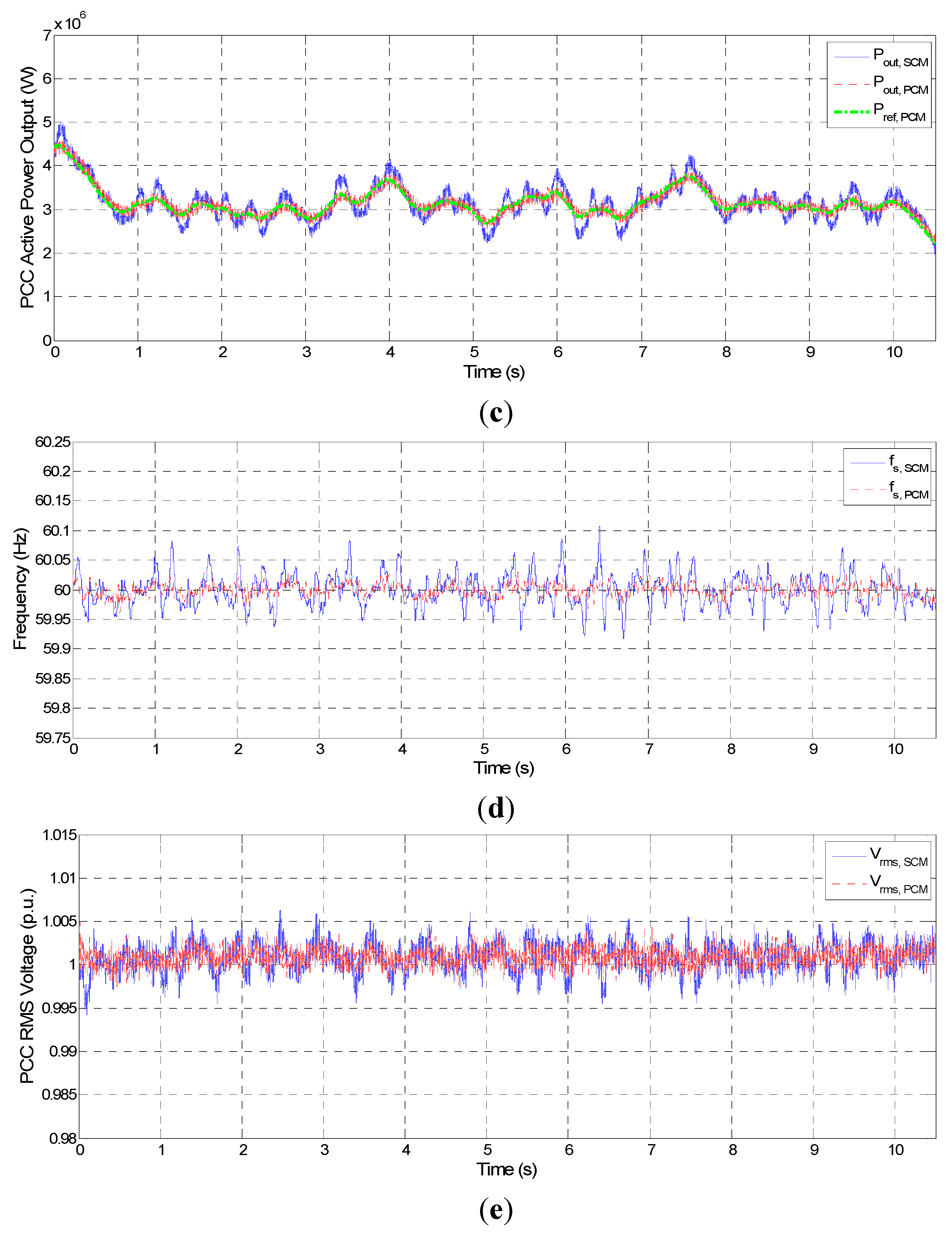
The simulated data for case 1 are shown in Figure 8. The power coefficient and power quality of SCM and PCM were slightly different when the wind-speed fluctuation was weak. Figure 8a shows ${\omega }_{e,SCM}$, ${\omega }_{e,PCM}$, and ${\omega }_{e,opt}$ for case 1; ${\omega }_{e,SCM}$ followed ${\omega }_{e,opt}$ slightly faster than ${\omega }_{e,PCM}$ did.

Figure 8. Simulated data for case 1. (a) Electrical rotor speed; (b) power coefficient; (c) active power output at the PCC; (d) frequency at the PCC; and (e) RMS voltage at the PCC.

Figure 8. Simulated data for case 1. (a) Electrical rotor speed; (b) power coefficient; (c) active power output at the PCC; (d) frequency at the PCC; and (e) RMS voltage at the PCC.

This means that SCM exhibited better performance than PCM in terms of efficiency, which can be verified from Figure 8b. However, from the power quality and system stability point of view, PCM exhibited more steady operation than SCM.

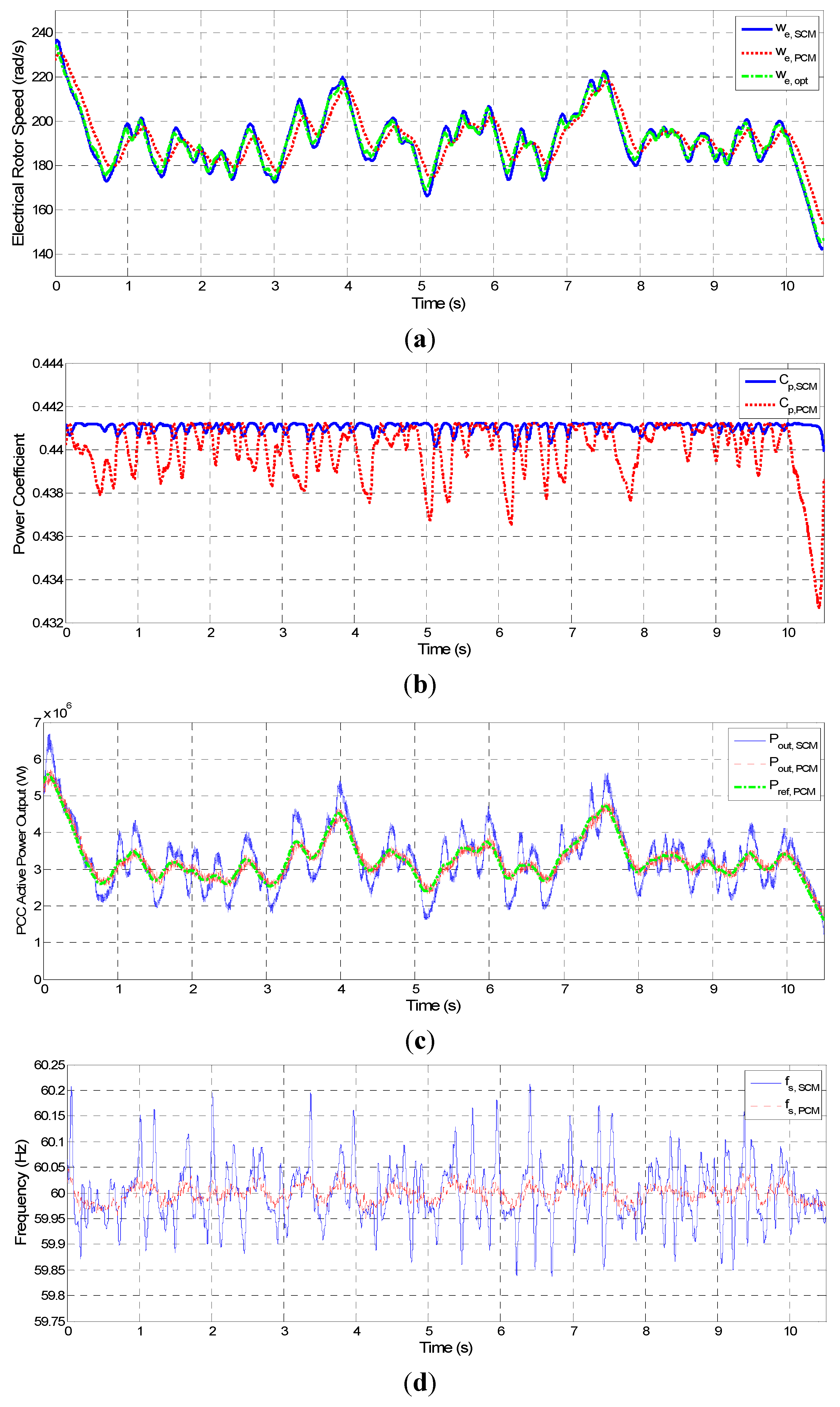
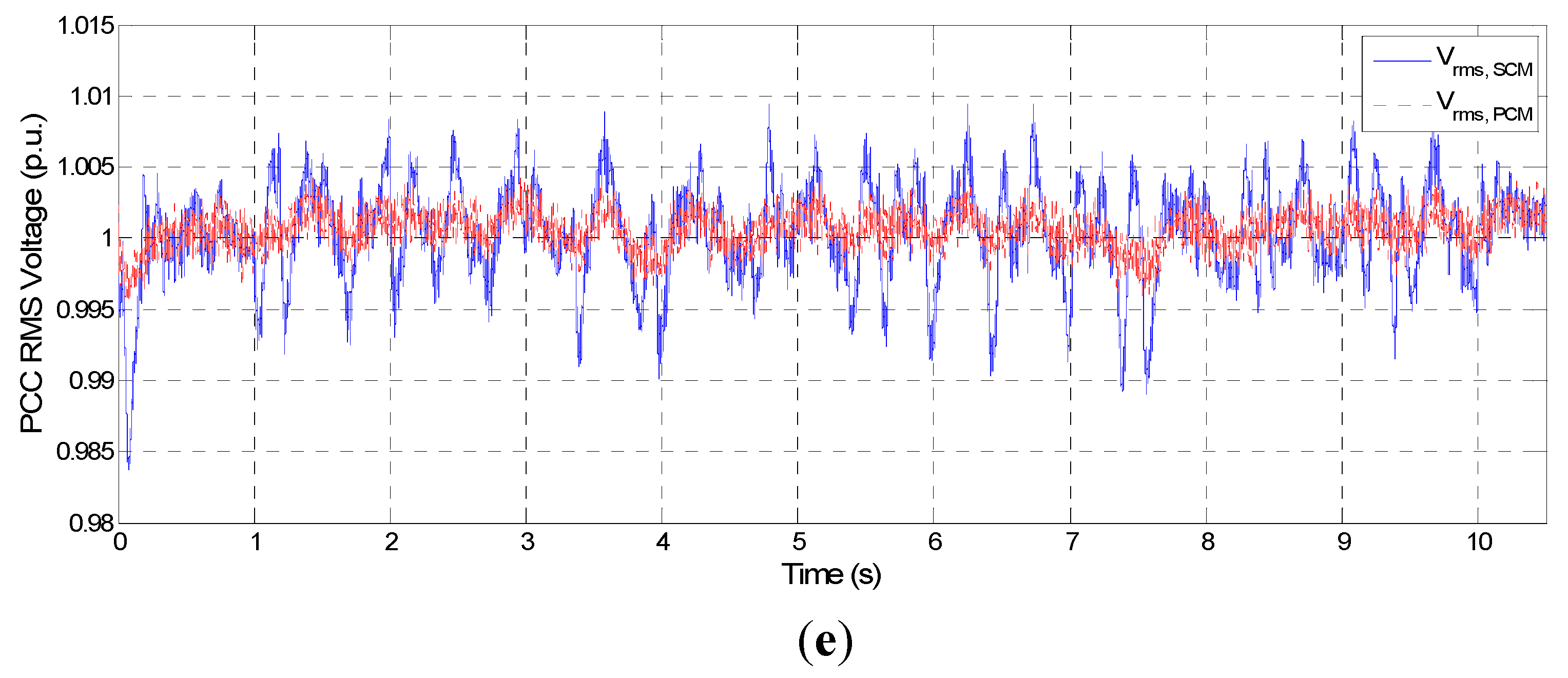
These differences between the two modes became more obvious as the wind-speed fluctuations increased. Figure 9a shows that as the rate and magnitude of the changes in wind speed became larger, the corresponding optimal rotor speed changed more rapidly. This became too fast for PCM to adjust ${\omega }_{e,PCM}$ in response to ${\omega }_{e,opt}$ due to the time delay of the PCM controller, while SCM adjusted ${\omega }_{e,SCM}$ in response to changes in ${\omega }_{e,opt}$ despite the intensified wind-speed fluctuations. Consequently, the efficiency gap between the two control modes increased. On the other hand, the power fluctuations, frequency deviation, and voltage deviation were more significant with SCM than with PCM. Thus, PCM is preferable from a power quality and system stability perspective.

Figure 9. Simulated data for case 2. (a) Electrical rotor speed; (b) power coefficient; (c) active power output at the PCC; (d) frequency at the PCC; and (e) RMS voltage at the PCC.

Figure 9. Simulated data for case 2. (a) Electrical rotor speed; (b) power coefficient; (c) active power output at the PCC; (d) frequency at the PCC; and (e) RMS voltage at the PCC.

3.2. Discussion

Table 4 shows the average of $C_p$ and $C_{p,av{g}_{,}}$ as well as the maximum deviation from $C_{p,max}$ and $\mathrm{\Delta }{C}_{p,max}$, for each case to provide a numerical analysis of the relative efficiencies of SCM and PCM.

Table 4. Numerical comparison of the power coefficients of the three cases.

Control Mode	Case 1		Case 2
	$C_{p,avg}$	$\Delta C_{max}$	$C_{p,avg}$	$\Delta C_{max}$
SCM	0.4412	0.0003	0.4410	0.0012
PCM	0.4409	0.002	0.4400	0.0085

Table 4. Numerical comparison of the power coefficients of the three cases.

Control Mode	Case 1		Case 2
	$C_{p,avg}$	$\Delta C_{max}$	$C_{p,avg}$	$\Delta C_{max}$
SCM	0.4412	0.0003	0.4410	0.0012
PCM	0.4409	0.002	0.4400	0.0085

For case 1, if wind-speed fluctuations occur, $C_{p,avg}$ of SCM is maintained close to $C_{p,max}$. On the other hand, with PCM, $C_{p,avg}$ fell below $C_{p,max}$ to 0.4409. This means that if PCM is used as the active power-control mode of a VSWT, an average active power loss of 0.453% will occur relative to the optimal value, while SCM maintains the optimal output power. In case 2, the average active power losses of SCM and PCM were 0.272% and 1.927%, respectively. Thus, SCM is preferable to PCM in terms of efficiency, and the gap between the two modes increases when the wind-power fluctuations are more significant.

It appears that SCM offers significantly better performance than PCM if efficiency is the only concern. However, from a system stability and power quality perspective, PCM is superior to SCM, as indicated by the data listed in Table 5 and Table 6. The maximum frequency deviation, $\mathrm{\Delta }{f}_{max}$, from the nominal value is shown in Table 5; in case 2, this was approximately two times larger than in case 1 when the VSWT was controlled using SCM. In contrast, when using PCM, the difference in $\mathrm{\Delta }{f}_{max}$ was less than a factor of two between cases 1 and 2. Moreover, $\mathrm{\Delta }{V}_{max}$, the maximum RMS voltage deviation from the nominal value, changed little for the two cases when the VSWT was controlled by PCM, while it changed dramatically when the VSWT was controlled using SCM.

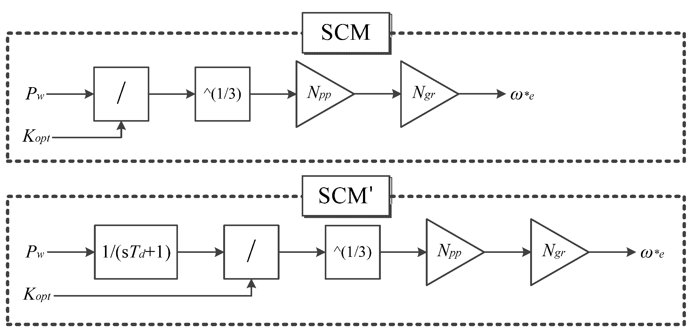
However, it may be arguable in the point of view that SCM can be controlled as similar as PCM in power quality perspective. For instance, it can be implemented by using time delay function before ${\omega }_e^{*}$ of SCM as shown in Figure 10, where $T_d$ is the time constant of the time delay function.

Table 5. Numerical comparison of the system frequencies of the three cases.

Control Mode	Case 1 (Hz)			Case 2 (Hz)
	$f_{s,min}$	$f_{s,max}$	${\Delta }{f}_{max}$	$f_{s,min}$	$f_{s,max}$	${\Delta }{f}_{max}$
SCM	59.9170	60.1070	0.1070	59.8377	60.2199	0.2199
PCM	59.9613	60.0301	0.0387	59.9457	60.0469	0.0543

Table 5. Numerical comparison of the system frequencies of the three cases.

Control Mode	Case 1 (Hz)			Case 2 (Hz)
	$f_{s,min}$	$f_{s,max}$	${\Delta }{f}_{max}$	$f_{s,min}$	$f_{s,max}$	${\Delta }{f}_{max}$
SCM	59.9170	60.1070	0.1070	59.8377	60.2199	0.2199
PCM	59.9613	60.0301	0.0387	59.9457	60.0469	0.0543

Table 6. Numerical comparison of the RMS voltages of the three cases.

Control Mode	Case 1 (p.u.)			Case 2 (p.u.)
	$V_{min}$	$V_{max}$	${\Delta }{V}_{max}$	$V_{min}$	$V_{max}$	${\Delta }{V}_{max}$
SCM	0.9942	1.0063	0.0063	0.9838	1.0095	0.0162
PCM	0.9974	1.0050	0.0050	0.9958	1.0045	0.0045

Table 6. Numerical comparison of the RMS voltages of the three cases.

Control Mode	Case 1 (p.u.)			Case 2 (p.u.)
	$V_{min}$	$V_{max}$	${\Delta }{V}_{max}$	$V_{min}$	$V_{max}$	${\Delta }{V}_{max}$
SCM	0.9942	1.0063	0.0063	0.9838	1.0095	0.0162
PCM	0.9974	1.0050	0.0050	0.9958	1.0045	0.0045

Figure 10. Methods of giving ${\omega }_e^{*}$ signal to speed controller.

Figure 10. Methods of giving ${\omega }_e^{*}$ signal to speed controller.

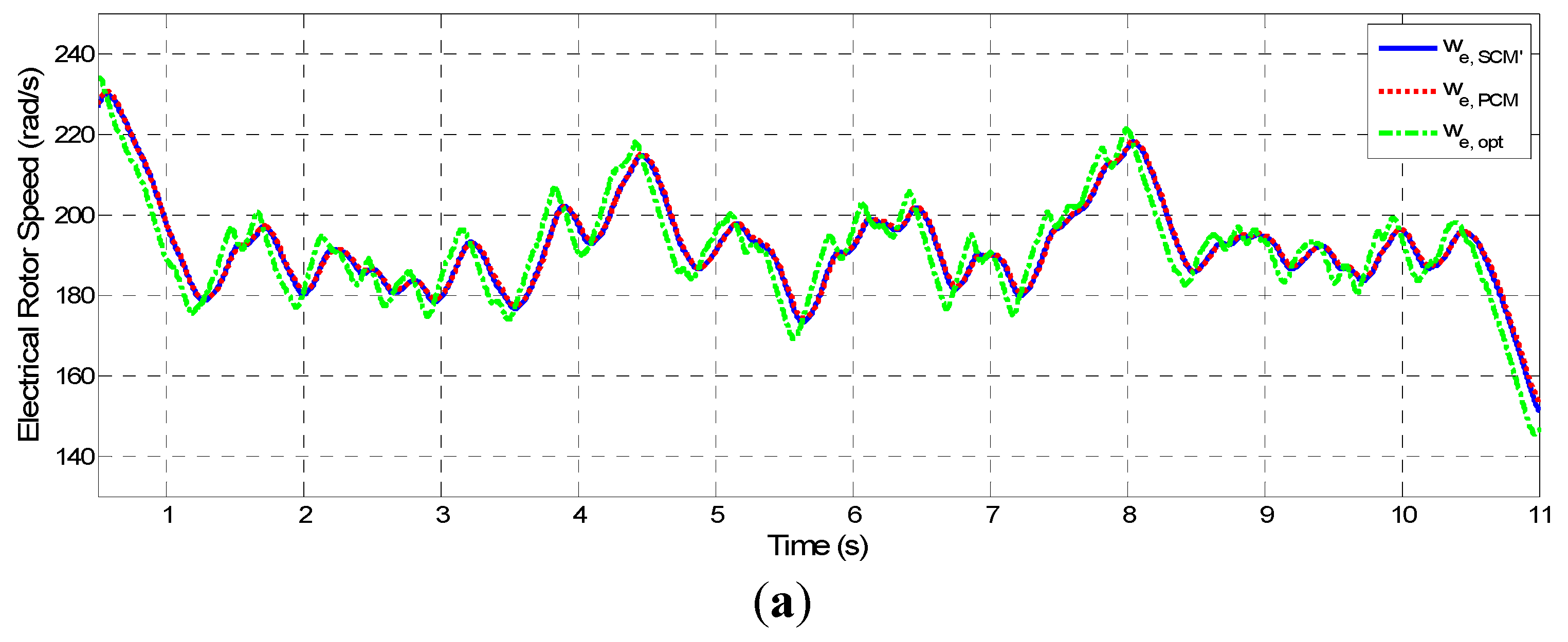
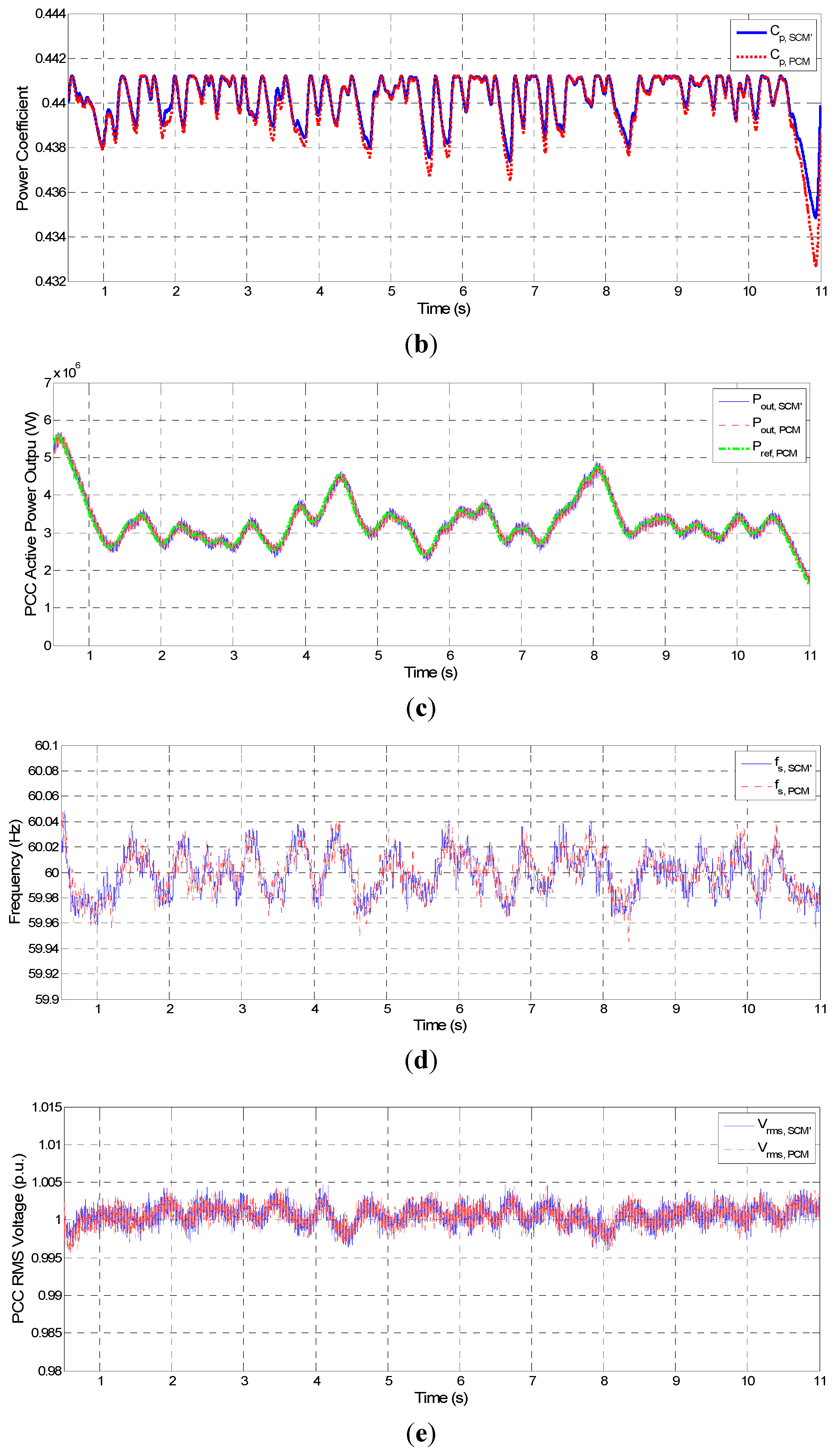
Since SCM′ is suggested to improve power quality, it may be compared with PCM as shown in Figure 11. $T_d$ is given as 0.1 s. From Figure 11a, it can be noticed that ${\omega }_e$ of both SCM′ and PCM are slightly deviated from ${\omega }_{e,opt}$, and as a result, power coefficients of both methods are deviated from $C_{p,max}$. Besides, power quality of SCM′ is similar to that of PCM as shown by Figure 11c–e. This proves that SCM can be controlled as similar as PCM in power quality point of view. However, it is hard to determine the value of $T_d$ to make performance of electrical signals of SCM as same as those of PCM, and still, SCM′ is slightly superior to PCM in power coefficient perspective as can be shown in Figure 11b.

Figure 11. Comparison between SCM′ and PCM. (a) Electrical rotor speed; (b) power coefficient; (c) active power output at the PCC; (d) frequency at the PCC; and (e) RMS voltage at the PCC.

Figure 11. Comparison between SCM′ and PCM. (a) Electrical rotor speed; (b) power coefficient; (c) active power output at the PCC; (d) frequency at the PCC; and (e) RMS voltage at the PCC.

4. Conclusions

We compared two control modes of wind turbines using MPPT; SCM adjusts the rotor speed and PCM adjusts the active power. Most of the previous work has considered only one of these in the control loop, regardless of the objectives, which are typically power quality, system stability, and efficiency. We carried out simulations to investigate the differences between the two control methods in the presences of wind-speed fluctuations.

Two cases were investigated with various magnitudes of wind-speed fluctuations using both SCM and PCM. Although it is not tested by simulation, it is obvious that with constant wind speed, the two control mechanisms were identical. However, when the wind-speed fluctuations increased in magnitude, differences appeared between the two control methods. We concluded that SCM is preferable to PCM in terms of the power coefficient and therefore yields slightly higher power output, whereas PCM is superior in terms of power quality and system stability, yielding a more stable electricity signal. The method of applying time delay function to SCM to make it as similar as PCM in power quality point of view is investigated. Although power quality can be improved by this method, SCM still has superiority to PCM in power coefficient perspective. These results can be used as a reference by wind-farm operators to determine the optimum control mode of VSWTs depending on the magnitude of the wind-speed fluctuations and on their operational goal, whether to maximize power output or the quality of the output signal. However, since the VSWT used in this simulation is full-converter WT, the results can be applied only to WTs equipped with full-converter and not to other types of VSWT such as DFIGs.

References

1. Global Wind Energy Council. Global Wind Energy Outlook 2012; Global Wind Energy Council: Brussels, Belgium, 2012. Available online: http://www.gwec.net/wp-content/uploads/2012/11/GWEO_2012_lowRes.pdf (accessed on 5 June 2013).
2. Iglesias, R.L.; Arantegui, R.L.; Alonso, M.A. Power electronics evolution in wind turbines—A market-based analysis. Renew. Sustain. Energy Rev. 2011, 15, 4982–4993. [Google Scholar] [CrossRef]
3. Ackermann, T. Wind Power in Power Systems; John Wiley & Sons: Hoboken, NJ, USA, 2005. [Google Scholar]
4. Tsili, M.A.; Papathanassiou, S.A. A review of grid code technical requirements for wind farms. IET Renew. Power Gener. 2009, 3, 308–332. [Google Scholar] [CrossRef]
5. Teodorescu, R.; Liserre, M.; Rodríguez, P. Grid Converters for Photovoltaic and Wind Power Systems; John Wiley & Sons: Hoboken, NJ, USA, 2011. [Google Scholar]
6. Uehara, A.; Pratap, A.; Goya, T.; Senjyu, T.; Yona, A.; Urasaki, N.; Funabashi, T. A coordinated control method to smooth wind power fluctuations of a PMSG-based WECS. IEEE Trans. Energy Convers. 2011, 26, 550–558. [Google Scholar] [CrossRef]
7. Qu, L.; Qiao, W. Constant power control of DFIG wind turbines with supercapacitor energy storage. IEEE Trans. Ind. Appl. 2011, 47, 359–367. [Google Scholar] [CrossRef]
8. Teleke, S.; Baran, M.E.; Huang, A.Q.; Bhattacharya, S.; Anderson, L. Control strategies for battery energy storage for wind farm dispatching. IEEE Trans. Energy Convers. 2009, 24, 725–732. [Google Scholar] [CrossRef]
9. Morren, J.; de Haan, S.W.H.; Kling, W.L.; Ferreira, J.A. Wind turbines emulating inertia and supporting primary frequency control. IEEE Trans. Power Syst. 2006, 21, 433–434. [Google Scholar] [CrossRef]
10. Conroy, J.F.; Watson, R. Frequency response capability of full converter wind turbine generators in comparison to conventional generation. IEEE Trans. Power Syst. 2008, 23, 649–656. [Google Scholar] [CrossRef]
11. Chang-Chien, L.R.; Lin, W.T.; Yin, Y.C. Enhancing frequency response control by DFIGs in the high wind penetrated power systems. IEEE Trans. Power Syst. 2011, 26, 710–718. [Google Scholar] [CrossRef]
12. Wang, X.; Wu, S. Nonlinear Dynamic Modeling and Numerical Simulation of the Wind Turbine’s Gear Train. In Proceedings of the 2011 International Conference on Electrical and Control Engineering, Yichang, China, 16 September–18 September 2011; pp. 2385–2389.
13. Chang-Chien, L.R.; Yin, Y.C. Strategies for operating wind power in a similar manner of conventional power plant. IEEE Trans. Energy Convers. 2009, 24, 926–934. [Google Scholar] [CrossRef]
14. Luo, C.; Bankar, H.; Shen, B.; Ooi, B.T. Strategies to smooth wind power fluctuations of wind turbine generator. IEEE Trans. Energy Convers. 2007, 22, 341–349. [Google Scholar] [CrossRef]
15. Morren, J.; Pierik, J.; de Haan, S.W.H. Inertial response of variable speed wind turbines. Electr. Power Syst. Res. 2006, 76, 980–987. [Google Scholar] [CrossRef]
16. Bankar, H.; Luo, C.; Ooi, B.T. Steady-state stability analysis of doubly-fed induction generators under decoupled P-Q control. IEE Proc. Electr. Power Appl. 2006, 153, 300–306. [Google Scholar] [CrossRef]
17. Yazdani, A.; Iravani, R. A neutral-point clamped converter system for direct-drive variable-speed wind power unit. IEEE Trans. Energy Convers. 2006, 21, 596–607. [Google Scholar] [CrossRef]