Comparative Study of Dynamic Programming and Pontryagin’s Minimum Principle on Energy Management for a Parallel Hybrid Electric Vehicle

Abstract
:1. Introduction
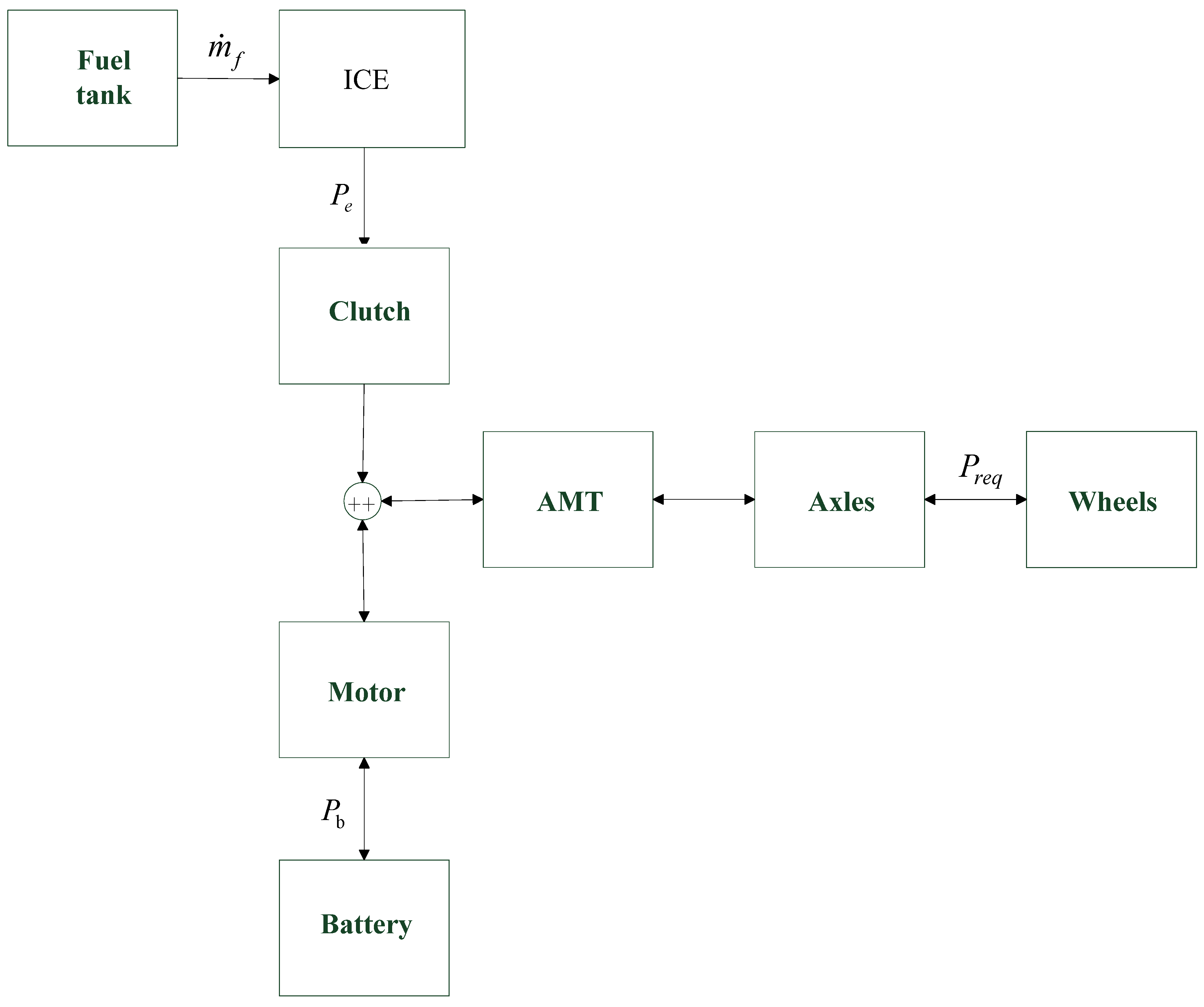
2. Hybrid Powertrain Modeling


3. Application of DP and PMP
3.1. The DP-Based Numerical Optimization
 , which results in:

3.2. The PMP-Based Optimization
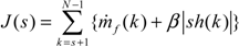
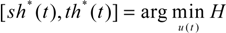
- The u*(t) minimizes the Hamiltonian H(x(t), u(t), t, p(t)) for all :where the Hamiltonian is defined as:
![Energies 06 02305 i007]() With p(t) is a vector of the auxiliary variables called co-states and the dimension of p(t) is the same as x(t).
With p(t) is a vector of the auxiliary variables called co-states and the dimension of p(t) is the same as x(t).![Energies 06 02305 i008]()
- The co-state p(t) satisfies the following equation:
![Energies 06 02305 i009]()
- The terminal condition is similar to Equation (12).


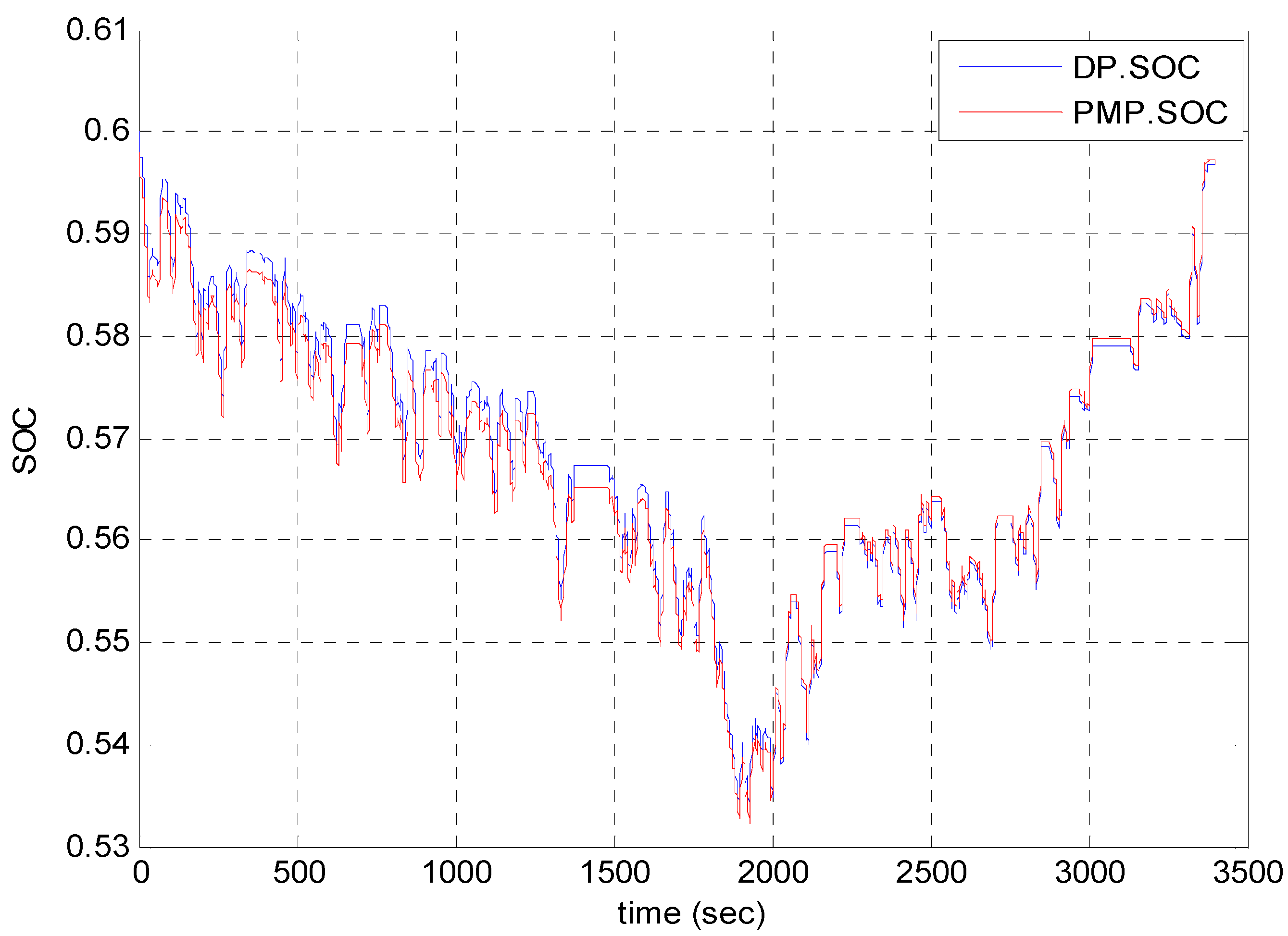
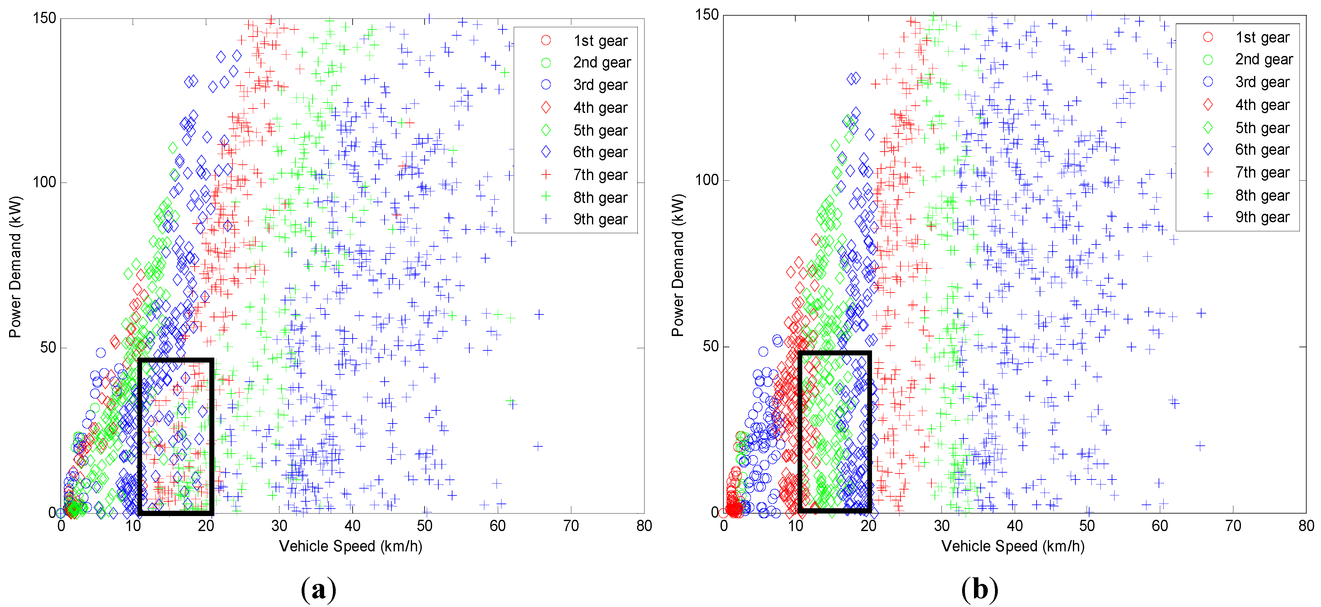
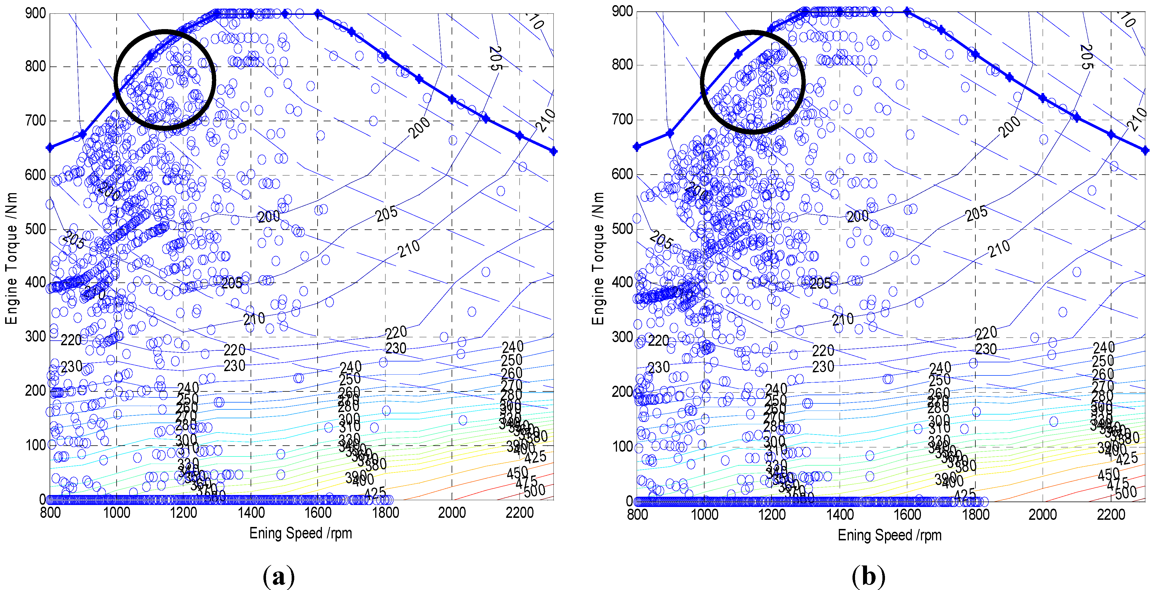
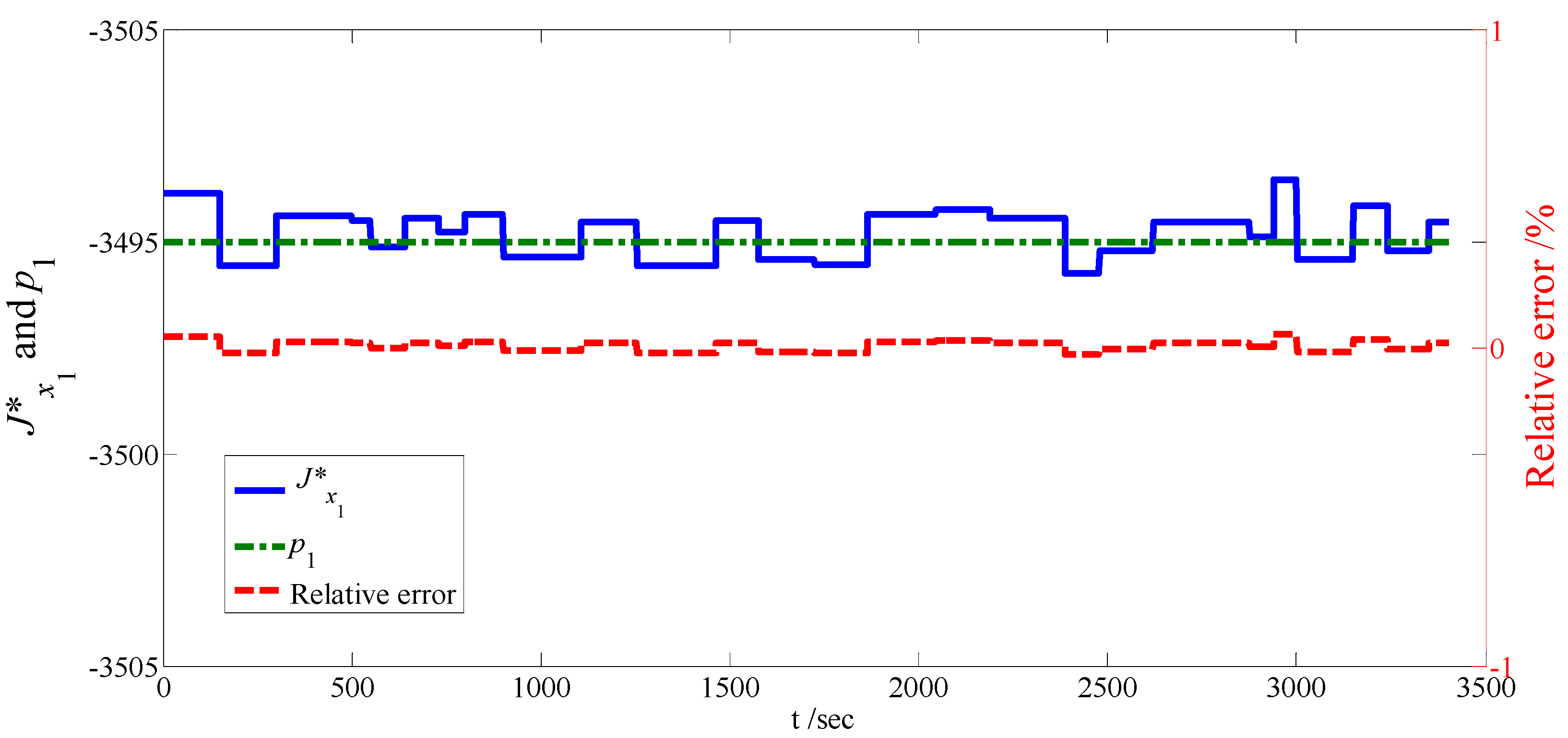
4. Comparative Analysis for the Results from PMP and DP

5. Conclusions
Acknowledgements
References
- Sciarretta, A.; Guzzella, L. Control of hybrid electric vehicles. IEEE Control Syst. Mag. 2007, 27, 60–70. [Google Scholar] [CrossRef]
- Serrao, L.; Onori, S.; Rizzoni, G.; Guezennec, Y. A Novel Model-Based Algorithm for Battery Prognosis. In Proceedings of the Seventh IFAC Symposium on Fault Detection, Supervision and Safety of Technical Processes, Barcelona, Spain, 30 June–3 July 2009.
- Brahma, A.; Guezennec, Y.; Rizzoni, G. Optimal Energy Management in Series Hybrid Electric Vehicles. In Proceedings of the 2000 American Control Conference, Columbus, OH, USA, 28–30 June 2000; pp. 60–64.
- Lin, C.-C.; Peng, H.; Grizzle, J.W.; Kang, J.-M. Power management strategy for a parallel hybrid electric truck. IEEE Trans. Control Syst. Technol. 2003, 11, 839–849. [Google Scholar] [CrossRef]
- Sundström, O.; Ambühl, D.; Guzzella, L. On implementation of dynamic programming for optimal control problems with final state constraints. Oil Gas Sci. Technol. 2009, 65, 91–102. [Google Scholar] [CrossRef]
- Anatone, M.; Cipollone, R.; Sciarretta, A. Control-Oriented Modeling and Fuel Optimal Control of a Series Hybrid Bus; SAE Technical Paper 2005-01-1163; SAE International: Warrendale, PA, USA, 2005. [Google Scholar] [CrossRef]
- Wei, X.; Guzzella, L.; Utkin, V.; Rizzoni, G. Model-based fuel optimal control of hybrid electric vehicle using variable structure control systems. J. Dyn. Syst. Meas. Control 2007, 129, 13–19. [Google Scholar] [CrossRef]
- Serrao, L.; Rizzoni, G. Optimal Control of Power Split for a Hybrid Electric Refuse Vehicle. In Proceedings of the 2008 American Control Conference, Seattle, WA, USA, 11–13 June 2008; pp. 4498–4503.
- Johannesson, L.; Åsbogård, M.; Egardt, B. Assessing the potential of predictive control for hybrid vehicle powertrains using stochastic dynamic programming. IEEE Trans. Intell. Transp. Syst. 2007, 8, 71–83. [Google Scholar] [CrossRef]
- Tate, E.; Grizzle, J.; Peng, H. Shortest path stochastic control for hybrid electric vehicles. Int. J. Robust Nonlinear Control 2008, 18, 1409–1429. [Google Scholar] [CrossRef]
- Borhan, H.; Vahidi, A.; Phillips, A.; Kuang, M.; Kolmanovsky, I. Predictive Energy Management of a Power-Split Hybrid Electric Vehicle. In Proceedings of the 2009 American Control Conference, St. Louis, MO, USA, 10–12 June 2009.
- Jeon, S.I.; Jo, S.T.; Park, Y.I.; Lee, J.M. Multi-mode driving control of a parallel hybrid electric vehicle using driving pattern recognition. J. Dyn. Syst. Meas. Control 2002, 124, 141–149. [Google Scholar] [CrossRef]
- Delprat, S.; Guerra, T.M.; Rmaux, J. Control Strategies for Hybrid Vehicles: Optimal Control. In Proceedings of Vehicular Technology Conference, 2002 (VTC 2002-Fall), Vancouver, Canada, 24–28 September 2002; pp. 1681–1685.
- Delprat, S.; Lauber, J.; Marie, T.; Rimaux, J. Control of a paralleled hybrid powertrain: Optimal control. IEEE Trans. Veh. Technol. 2004, 53, 872–881. [Google Scholar] [CrossRef]
- Rousseau, G.; Sinoquet, D.; Rouchon, P. Constrained optimization of energy management for a mild-hybrid vehicle. Oil-Gas Sci. Technol. IFP 2007, 62, 623–624. [Google Scholar] [CrossRef]
- Cipollone, R.; Sciarretta, A. Analysis of the Potential Performance of a Combined Hybrid Vehicle with Optimal Supervisory Control. In Proceedings of the 2006 IEEE International Conference on Control Applications, Munich, Germany, 4–6 October; pp. 2802–2807.
- Sciarretta, A.; Back, M.; Guzzella, L. Optimal control of paralleled hybrid electric vehicles. IEEE Trans. Control Syst. Technol. 2004, 12, 352–363. [Google Scholar] [CrossRef]
- Guzzella, L.; Sciarretta, A. Vehicle Propulsion Systems: Introduction to Modeling and Optimization; Springer-Verlag: Berlin, Germany, 2005; pp. 208–225. [Google Scholar]
- Musardo, C.; Rizzoni, G.; Guezennec, Y.; Staccia, B. A-ECMS: An adaptive algorithm for hybrid electric vehicle energy management. Eur. J. Control 2005, 11, 509–524. [Google Scholar] [CrossRef]
- Serrao, L.; Onori, S.; Rizzoni, G. A comparative analysis of energy management strategies for hybrid electric vehicles. J. Dyn. Syst. Meas. Control 2011, 133, 031012:1–031012:9. [Google Scholar] [CrossRef]
- Kim, N.; Cha, S.; Peng, H. Optimal control of hybrid electric vehicles based on Pontryagin’s minimum principle. IEEE Trans. Control Syst. Technol. 2011, 19, 1279–1287. [Google Scholar] [CrossRef]
- Zou, Y.; Hou, S.J.; Li, D.G.; Gao, W.; Hu, X.S. Optimal energy control strategy design for a hybrid electric vehicle. Discret. Dyn. Nat. Soc. 2013. [Google Scholar] [CrossRef]
- Kirk, D.E. Optimal Control Theory: An Introduction; Dover Publications Incorporated: Mineola, NY, USA, 2004; pp. 227–240. [Google Scholar]
- Krotov, V.F. Global Methods in Optimal Control Theory; Marcel Dekker, Inc: New York, NY, USA, 1996; p. 140. [Google Scholar]
© 2013 by the authors; licensee MDPI, Basel, Switzerland. This article is an open access article distributed under the terms and conditions of the Creative Commons Attribution license (http://creativecommons.org/licenses/by/4.0/).
Share and Cite
Yuan, Z.; Teng, L.; Fengchun, S.; Peng, H. Comparative Study of Dynamic Programming and Pontryagin’s Minimum Principle on Energy Management for a Parallel Hybrid Electric Vehicle. Energies 2013, 6, 2305-2318. https://doi.org/10.3390/en6042305
Yuan Z, Teng L, Fengchun S, Peng H. Comparative Study of Dynamic Programming and Pontryagin’s Minimum Principle on Energy Management for a Parallel Hybrid Electric Vehicle. Energies. 2013; 6(4):2305-2318. https://doi.org/10.3390/en6042305
Chicago/Turabian StyleYuan, Zou, Liu Teng, Sun Fengchun, and Huei Peng. 2013. "Comparative Study of Dynamic Programming and Pontryagin’s Minimum Principle on Energy Management for a Parallel Hybrid Electric Vehicle" Energies 6, no. 4: 2305-2318. https://doi.org/10.3390/en6042305