1. Introduction
The current electricity grid is a product of decades of development and evolution, serving its primary goal of reliably delivering electricity to the masses. Recently, there has been a concerted push to modernize the electricity grid and introduce new energy resources, requiring the integration of modern communication technologies to allow for better communication and information flow between grid operators, utilities and consumers [
1,
2,
3,
4,
5,
6,
7,
8,
9]. This new paradigm of electricity distribution will allow for better load balancing between suppliers and consumers and even allow for some degree of demand shaping. This potential in demand management is generating huge interest in research, generating a fast growing body of work.
The amount of electricity that needs to be produced by energy producers in order to meet consumer demands in a residential sector varies temporally. These temporal variations in electricity demand result from varying power consumption and scheduling requirements of electrical appliances (loads/devices) of different consumers. In a traditional power grid, all the electrical appliances are managed by each user according to his/her preferred scheduling times, e.g., a user might prefer clothes drying early in the morning, while someone else prefers to do the same task in the evening. The electricity grid is then required to deliver electricity to match this demand. In a future smart grid, this relationship may change. In such smart grid system, consumers might be persuaded (maybe through proper motivations/incentives) by the grid to allow certain tasks, which are not essential, to become flexible in their operation. A user might then shift some of its flexible loads in order to achieve a more steady (flat) demand profile for the benefit of the electricity grid. This scheduling flexibility may however, result in more inconvenience to users.
1.1. Motivation
The objective of our paper is to study the impact of scheduling flexibility on demand profile flatness and user inconvenience. Through this study, we can understand how much demand profile flatness can be achieved and how much inconvenience is experienced by users if their loads are re-scheduled by a certain amount. A user can change the schedule of its tasks and participate in demand response only if proper incentives are offered by the grid to compensate for the resulting inconvenience. In many previous works, dynamic pricing model is often used as an incentive for demand shaping [
10,
11,
12,
13,
14,
15]. The most widely used dynamic pricing model in literature is a two-tier pricing model (where according to time of use different prices are charged). Some authors have used linear or quadratic functions to reflect the dynamic price. Real-time pricing (RTP) is also considered in some papers. In all such formulations, dynamic energy price is an incentive that is offered by the grid and assumed to be accepted by the users. The reason why some dynamic pricing function should be adopted by the grid and accepted by the users is not specified. The questions, e.g., “is it the appropriate dynamic pricing function to meet the objectives of the grid?" or “is it the appropriate dynamic pricing function that will result in the required amount of user participation to meet the required objectives?" or “is it the best dynamic pricing function for a user to accept it and motivate him for demand response?" are never answered. Therefore, in order to come up with proper incentives, it is extremely crucial that the grid should know how much it can gain from causing inconvenience to users and what should be the user participation rate in order to obtain specific demand response objectives. Similarly, the users should also need to know how much inconvenience they will experience for a given incentive provided by the grid.
1.2. State of the Art
The objective of this paper is to understand and quantify the impact of scheduling flexibility in load on both demand profile flatness and user inconvenience in residential smart grid systems. There are some recent studies on this problem. The authors in [
14] propose a game-theoretic approach for scheduling home appliances. This method proposes the consumer perspective of the problem where the users always want to schedule their loads for hours when the price is low. However, the side-effect of this algorithm is a shift in peak load without any significant peak reduction. To mitigate this problem, the authors propose to use RTP. However, they fail to consider and quantify the impact of this re-scheduling onto the grid and user inconvenience. In [
15], the authors propose the use of RTP by the utility company as a demand response program in smart grid. This would result in reduced power consumption during peak hours. The objective is to optimize the shiftable load scheduling to minimize the power consumption cost using a constrained Markov decision process model. By using the RTP, the grid is able to reduce its inconvenience but no discussion is provided on the quantification of the user inconvenience. In [
16] the authors design incentives and propose scheduling algorithms considering strictly convex functions of costs. Users are given incentives to move to off peak hours and these incentives are proposed using game theoretic analysis. However they do not consider or quantify the inconvenience levels of the users. The authors in [
17] propose a Stackelberg game between operators and consumers. This game allows operators to determine optimal electricity price and consumers their optimal power consumption. In [
18] authors propose a pricing scheme for users in order to achieve a perfectly flat demand curve. They show that finding an optimum schedule is a NP-hard problem. They propose centralized and distributed algorithms depending on the degree of knowledge of the state of the network. In [
19], the author propose a framework for demand response in smart grids that integrates renewable distributed generators (DGs). In this model, some users have DGs that help partially accommodating their electricity needs. The users can also sell additional generated electricity to the utility company. The authors demonstrate through numerical examples that their distributed algorithm is able to achieve significant reduction in the peak-hour load and costs to the utility and users with significantly reduced computation cost. However, the work again does not consider or quantify the user inconvenience caused due to rescheduling of load from peak hours. The authors in [
20] propose a strategy to achieve a uniform power consumption over time. Their algorithm schedules the devices in such a way that a target power level is not exceeded in each time slot. Again, the authors do not take into account the inconvenience level of users while designing these algorithms. In [
21] the authors use convex optimization tools and solve a cooperative scheduling problem in a smart grid. The authors in [
22] used a water-filling based scheduling algorithm to obtain a flat demand curve. The proposed algorithm does not require any communication between scheduling nodes. The authors also study the possible errors in demand forecast and incentives for customer participation. The authors in [
23] presented demand side management strategies for a large number of household appliances of several types using heuristic optimization techniques. In [
24] the authors consider load shifting, introduce another management strategy through manipulating throttle-able appliances. These appliances are defined as appliances which have a fixed operational period but flexible power consumption pattern. The authors in [
25] provide a comprehensive survey of the demand side management (DSM) that covers the taxonomy for DSM, analyzes the various types of DSM, and gives an outlook on the latest demonstration projects in this domain. However, it misses the grid side perspective of the problem.
It should be noted that the objectives of most of these studies are to achieve a flat demand curve for the electricity grid. In other words, they are mostly looking at the reduction in grid inconvenience by offering some sorts of incentives to the users. However, they ignore to formulate or quantify the user inconvenience level that actually help forming an incentive based system for future grid. In our proposed work, we study the compromise between the grid objective of flat electricity demand vis-a-vis the inconvenience level of users. This is a significant problem as the acceptance of smart grid technologies by end users is one of the keys to the success of smart grid system.
1.3. Contributions
We formulate an optimization problem with the objective of minimizing peak load in the aggregated demand of several households in a residential smart grid system. This formulated optimization problem is NP-hard. We then develop optimal and greedy scheduling algorithms which are used to study the impact of scheduling flexibility variations in loads. We consider three variations of scheduling flexibility: delaying of loads, advance scheduling of loads, or a combination of both delaying and advance scheduling. We study the impact of these different flexibilities and duration of each type on the demand profile and user inconvenience. These scheduling algorithms can be implemented in a centralized, distributed or hybrid approach. In a centralized implementation, each consumer announces his/her set of appliances, their load consumption profiles, preferred time slots,
etc. to the Centralized Scheduler (CS), and the scheduling algorithm is executed by the CS. In a distributed implementation, there is no need for consumers to share these information with a CS (due to privacy concerns of consumers [
26,
27,
28]), and the scheduling algorithm is implemented individually at the level of the consumer. A hybrid distributed approach, here termed partially distributed implementation is also considered. In such an implementation, each consumer only needs to report its aggregated consumption over a certain period of time to the CS, and the CS will coordinate among the users. In such a partially distributed system, we show that the performance can approach a centralized performance while consumers need not report individual load info to the grid. We simulate the algorithms using practical load types and we have following important observations:
In the fully distributed case, when users are not willing to share any information with the CS, more scheduling flexibility is required (to achieve a certain amount of demand shaping) as compared to a centralized case.
In the partially distributed case, through the coordination of grid among multiple users on re-scheduling of flexible loads, the results can be comparable to the centralized case.
When more households participate, the grid operator can achieve a higher degree of flatness. However, the increase in user participation has diminishing returns for the grid in terms of demand shaping.
For a certain household participation rate, there exists a saturation point, and increasing scheduling flexibility beyond this saturation point does not significantly impact demand profile flatness.
Increasing user participation rate beyond a certain threshold does not impact the saturation point. We observed in our simulation setup that it is not possible to bring the saturation point down from 6 time slots even by increasing user participation from 50% to 100%.
1.4. Paper Organization
The rest of the paper is organized as follows. In
Section 2 we explain the system model, load model and formulate the optimization problem. In
Section 3 we discuss the solution and scheduling algorithm development.
Section 4 develops and explains the centralized and distributed implementations of scheduling algorithms. Simulation results are presented in
Section 5. The paper is concluded in
Section 6 and we discuss future work in
Section 7.
2. System Model, Load Model and Problem Formulation
2.1. System Model
We consider a residential smart grid system comprising of K households (also interchangeably called users or consumers throughout the paper) interacting with a system operator (also interchangeably called the grid) that manages the electricity generation and distribution network. Each household has a smart meter which is connected to a CS. We assume that in the centralized case, the smart meter gathers all the required information about consumer loads and their demand profiles and communicates it to CS. Any scheduling algorithm is executed by CS and the resulting demand profile flatness and user inconvenience levels are also measured by CS. In the distributed case, we assume that each user is equipped with its own scheduler which is used for the implementation of scheduling algorithms. In the partially distributed scenario, the CS exists to coordinate between the individual households. The resulting user inconvenience is also computed by the user and reported to the grid. Demand profile flatness is measured by the grid from the final aggregated load profile of all the users.
2.2. Load Model
The electrical load of each consumer can be classified into two types [
16,
29,
30]:
Essential load: These loads have fixed scheduling needs and cannot be re-scheduled. Refrigeration, watching television (TV), essential lighting are a few examples of such essential loads.
Flexible load: These loads have preferred scheduling times, however unlike essential loads these can be re-scheduled to other time slots.
Typically, each user has a limited number of loads (appliances) which can be declared as flexible. Typical flexible loads include Heating, Ventilation and Air conditioning (HVAC), Water Heating (WH), Clothes Drying (CD), Plug-In Hybrid Electrical Vehicles (PHEVs) and Optional Lighting (OL). Flexible load may be further categorized into several types, e.g., Thermostatically Controlled Loads (TCLs) (HVAC, WH) and shiftable loads (CD, PHEV). The power consumption of shiftable loads is not sensitive to scheduling variations. On the other hand, power consumption of TCLs in the presence of scheduling variations can be modeled in two different ways:
As fixed power consumption loads [
16,
29]: In this model, the power consumption of any TCL is assumed to be fixed and insensitive to scheduling variations. It is assumed that the objective is to achieve a constant thermostat reading and power variations in order to maintain fix thermostat reading are assumed to be insignificant.
As power throttling loads [
13,
24]: In this model, the power consumption of TCL can be varied within a certain range, e.g., [Power
, Power
]. Power variations result in temperature deviation from desired thermostat set point.
In this paper, we model TCLs as fixed power consumption loads. Without this assumption, different amount of scheduling flexibility will result in different total amount of power consumptions and it will become difficult to do a fair comparison of various schedules and their impact on demand profile flatness and user inconvenience. Thus our designed schedulers do not change the overall energy consumption but instead systematically manage and shift it according to the amount of scheduling flexibility. It should be noted here that operational constraints of TCL and their detailed thermodynamic model may also be incorporated in the optimization problem as additional constraints. Such formulation and modeling can capture the switching frequency and turn-on time and TCL duration correlations in different time slots. However, measuring the impact of these correlations on demand profile flatness and user inconvenience is not an easy task and is linked to the underlying thermal dynamic model for TCL (which is not unique).
We divide total time of a day (
h) into discrete time slots indexed by
t. The duration of each time slot can be an hour, half hour,
etc. Let,
denote the essential load of consumer
k in time slot
t. The essential load in time slot
t is obtained from the combination of essential load demands in period
t, e.g., if a user turns on essential lights from 7 pm to 8 pm and also watches TV in the same time duration, then his essential load in this time slot is the sum of these two loads. We assume that consumer
k has
flexible loads. We assume that
i-th flexible load of user
k requires
time slots to complete. We call
as the service time of flexible load
i of user
k. In this paper, we assume continuous operation of each flexible load until its completion. It means that if the flexible load is scheduled at time slot
, then it cannot be stopped and it will operate in consecutive time slots
. We assume that the electricity consumed by the flexible load
i of user
k if it is scheduled in time slot
M is given as:
where,
is the power consumption of flexible load
i of consumer
k. Each flexible load is assumed to have a preferred scheduling time slot denoted by
. The consumer enjoys the most convenience if the flexible load is scheduled at its most preferred time slot, e.g., for a certain consumer the most preferred time for CD might be at 1800 h, while for some other consumer the most preferred time slot for CD might be 2000 h. We consider a generalized framework, where we can introduce any type of scheduling flexibility in loads (delay only, advance scheduling only, or flexible in both delay and advance scheduling):
Delay (Post-loading): The operation of flexible loads can only be delayed. Re-scheduling can be done only after the most preferred time slot of a certain flexible load, e.g., use of optional lighting can be delayed.
Advance Scheduling (Pre-loading): The flexible loads can only be scheduled in advance, i.e., ahead of their most preferred time slot, e.g., air-conditioners turned on in advance to pre-cool the room before user’s preferred time slot.
Fully Flexible in both directions: In this case, flexible loads can be both delayed or advance scheduled depending on the requirements of the grid. Re-scheduling of a flexible load can be done on either side of its most preferred time slot, e.g., clothes drying can be done earlier than user’s preferred time slot or can be delayed.
We assume that the user suffers the same degree of inconvenience if its flexible load is shifted in either direction (before or after) of its most preferred time slot. In other words, delaying a flexible load by 2 time slots or advance scheduling the same load by 2 time slots will result in same amount of user inconvenience. In general, a scheduling flexibility of
X time slots in both directions will enable the scheduler to re-schedule flexible load
i of consumer
k between time slots,
. However, since we consider the scheduling problem in the interval
the re-scheduling has to be done in the interval
, where:
and
A flexible load
i of user
k cannot be re-scheduled before the first time slot
i.e.,
which means that it can only be advance scheduled in times slots
. Similarly the re-scheduling of flexible load
i of user
k cannot be delayed beyond
i.e.,
because otherwise this task could not be completed before
. Therefore, it can only be delayed to start in any of the time slots
. Depending on the type of scheduling flexibility we can define the scheduling interval denoted by
as follows:
Delay (Post-loading): In this case scheduling interval is defined as:
Since flexible load starts before the preferred time, the left limit of the scheduling interval
is set as
while the right limit of the scheduling interval is set according to amount of scheduling flexibility.
Advance Scheduling (Pre-loading): In this case, the scheduling interval is defined as:
Since flexible load cannot start after the preferred time, the right limit of the scheduling interval
is set as
while the left limit of the scheduling interval is set according to amount of scheduling flexibility.
Fully Flexible Schedule: In this case, the scheduling interval is defined as:
The load can be re-scheduled to either side of the preferred start time.
2.3. Problem Formulation
In this subsection, we formulate an optimization problem for the centralized case (the optimization problem for a distributed case can be easily derived from the centralized problem). Let
denote the combined essential load of
K consumers in time slot
t. For notational convenience, we denote flexible load
i of consumer
k and its parameters (service time, power consumption and preferred start time) by
,
and
. We formulate the optimization problem (for any amount and type of scheduling flexibility) as follows:
subject to
The objective of the optimization problem is to minimize the peak load in any given time slot t. Constraint (3) indicates that the sum of power demand of flexible load i of consumer k over the scheduling interval should be equal to its total power consumption. Constraint (4) indicates that flexible load i of consumer k can only be scheduled in consecutive time slots starting from t till . Moreover, flexible load i of consumer k can be re-scheduled in interval (depending on X and the type of flexibility). The scheduling interval is computed according to the type of scheduling flexibility introduced in flexible loads as explained previously.
The optimization problem for
k-th user in the distributed case can be formulated by considering only the load of this particular user. This problem is given as:
subject to
In the distributed case, each individual user considers only its own flexible and essential loads. All the constraints are same but apply only on to the flexible loads of user k.
In the next section, we will develop algorithms to solve these optimization problems.
3. Solution and Algorithm Development
The optimization Problems (2) and (5) minimize peak load by re-scheduling flexible loads away from their most preferred time slots. While minimizing peak load achieves demand profile flatness, we can also consider the minimization of scheduling deviation from preferred time slots of flexible loads. This consideration would reduce user inconvenience. Before we look at algorithm development for the solution of the optimization problems, we have to define two extreme schedules. These extreme schedules will help us in measuring the amount of demand profile flatness and amount of inconvenience suffered by a user from any other schedule.
Grid Convenient Schedule (GCS): This schedule allows us to measure the amount of demand profile flatness provided by any other schedule. For a given set of essential and flexible loads this schedule represents the best schedule from the perspective of the grid (so we name it GCS). This schedule can be obtained by adding load over all time slots and then dividing the entire load (essential and flexible of all users) by the total number of time slots
T. Let
denote the load in time slot
t. Then in GCS we have,
where,
is constant in each time slot
t. It is assumed that if the grid can achieve a constant demand profile in each time slot through re-scheduling consumer loads then it suffers zero inconvenience. Note that this schedule is not a practical schedule for any given set of essential and flexible loads because in this schedule essential load is also re-scheduled (which is not possible). However this schedule represents an ideal situation for the grid and allows us to measure the amount of demand profile flatness achieved by other schedules. Let,
denote the load scheduling vector, where
is the total re-scheduled load in time slot
t provided by the schedule. Let
denote the mean square deviation of any schedule from GCS (
) for a given amount of scheduling flexibility
X. We can measure this deviation as follows:
In general we can achieve a flatter demand profile at the expense of increasing user inconvenience.
User Convenient Schedule (UCS): This schedule allows us to measure the amount of inconvenience experienced by a user from any other schedule. This schedule is the preferred and most convenient schedule for a user (so we name it UCS). In UCS, all the flexible loads of a user are exactly scheduled at their most preferred time slots. We can determine this schedule by treating all flexible loads of a user as essential loads and then schedule each load at its most preferred time slot (this is what happens in a traditional grid; all flexible loads of a user are scheduled according to his/her preferences), e.g., if for flexible load
i of user
k the most preferred time slot is
and
then in UCS we schedule this flexible load exactly in the third time slot as follows:
We determine
and then the total scheduled load of user
k during time slot
t is given as:
We denote UCS of user
k as
. Let
denote the mean square deviation of any schedule from
k-th user UCS. This deviation can be measured as follows:
where,
is the re-scheduled load of user
k in time slot
t provided by the schedule. The aggregate user inconvenience is then given as:
The inconvenience metrics and as defined above is one possible way to capture demand profile flatness and user inconvenience. It should be noted that one can also define several other metrics. For example, for measuring user inconvenience, user preferences for re-scheduling their flexible loads might also be considered by assigning different weights. Some users might declare HVAC to be of highest priority, followed by WH, etc. Thus for such users re-scheduling HVAC will cause more inconvenience. Specific inconvenience metrics can then be developed to measure the impact of re-scheduling on net user inconvenience.
We will now develop algorithms for the formulated optimization problems. In general flexible loads have to be considered one after another for re-scheduling. Peak load depends on the sequence or order in which the loads are considered. Flexible loads can be arranged in a number of different ways, e.g., given I flexible loads (regardless of X), we can consider them for re-scheduling in possible ways. Therefore, finding the optimal solution of the Problem (2) becomes very difficult since the complexity increases exponentially as the number of flexible loads increase. We have the following result.
Theorem 1 The optimization Problem (2) is NP-hard.
Proof: We consider the special case of the defined problem, with only one user. Furthermore, we restrict that , and . We then prove that this special case is NP-hard by an induction from Multi-Processor Scheduling problem, which is a well-know NP-hard problem in the strong sense.
Multi-Processor Scheduling problem: We are given m identical machines in and n jobs in . Job has a processing time . The objective of Multi-Processor Scheduling problem is to assign jobs to the machines so as to minimize the maximum load of the machines.
Given an instance of Multi-Processor Scheduling Problem, we can construct an instance of the decision version of the above special case of the defined problem in polynomial time as follows. Let there be time slots that can be scheduled for tasks, there be shiftable tasks, and be the power consumed for the i-th task. Then, the load of the tasks scheduled at time t is equal to the load of the jobs assigned at the t-th machine. In other words, the objective of minimizing the maximum load at each time is to minimize the maximum working load assigned at each machine. Thus, the instance of Multi-Processor Scheduling problem is equivalent to an instance of the special case of the defined load balancing problem. To sum up, the defined load balancing problem is NP-hard.
Before we develop the optimal algorithm, we develop a Greedy Algorithm. This algorithm is optimal only for a given flexible load order. However, this algorithm will be very helpful not only in developing an optimal algorithm, but affect both centralized and distributed implementations of the system as well.
3.1. Greedy Algorithm
We develop a greedy algorithm algorithm for a general set of flexible loads given in some particular order. Greedy algorithms are often proposed for NP-hard problems (since such algorithms provide workable heuristics). However, there is no universal greedy solution which could be used for every NP-hard problem. In fact depending on the nature of the optimization problem, different greedy algorithms can be proposed. Our greedy algorithm is particularly suited to the optimization problem presented in our paper and it provides the best possible schedule for a given device order.
Let
I denote a set of flexible loads with service times denoted by
, preferred time slots denoted by
and power consumptions by
(these loads may belong to one user or several users and may be given in any specified order). We present this algorithm as Algorithm 1. In this algorithm for a given scheduling flexibility
X, for all the flexible loads we determine their respective scheduling intervals
in line 2. Flexible load
i can be re-scheduled in any time slot
. If flexible load
i is scheduled at time
t then it will be complete after
time slots. We obtain all possible schedules for flexible load
i with all possible start times in lines 4–8 of the algorithm. From all possible schedules, we select the one which minimizes the peak load in line 9 and declare it as the best schedule for flexible load
i. In line 10, we update the total load and consider the next flexible load
i.
| Algorithm 1 Greedy Algorithm |
| 1. Initialize: and . |
| 2. For the given value of X, find . |
| 3. For all , |
| 4. For all |
| 5. For |
| 6. |
| 7. End for |
| 8. End for |
| 9. |
| 10. |
| 11. End for |
3.2. Optimal Algorithm
The schedule obtained by the greedy algorithm does not optimize over every possible device order. Hence the greedy algorithm is not an optimal algorithm for the developed optimization Problems (2) and (5). The dependence of the optimal schedule on the order or sequence in which we consider flexible loads is further illustrated by the following simple example.
Example: Consider
time slots and
user. Suppose the essential load is given as
. Suppose there are two flexible loads with power consumption in each time slot given as
and
. There are two possible permutations: load 1 followed by load 2 or load 2 followed by load 1. In the first case (when we schedule load 1 followed by load 2), the final schedule is:
with a peak load of 5 in third time slot. In the second case when load 2 is scheduled before load 1 we obtain two possible schedules:
both of which are optimal for this flexible load order and give a peak load of 7 either in first or third time slots. Therefore in order to reduce the peak load, it is optimal to schedule load 1 before scheduling load 2 (the sequence in which we consider flexible loads in general cannot be ignored).
Despite the fact that the optimization problem is NP-hard we can still develop an optimal algorithm with the help of the Greedy algorithm to find the optimal schedule for any given value of
X. The optimal algorithm can only be used if the number of flexible devices is low. Normally the number of flexible loads in each household does not exceed 4 or 5 (e.g., HVAC, WH, CD, PHEV and OL). Again this optimal algorithm can by employed by individual users in a distributed implementation or by the CS in a centralized implementation. Like the greedy algorithm, we develop this algorithm for a general case of
I flexible loads (its implementation in distributed and centralized cases will be explained later). There are
possible ways of arranging these flexible loads. The optimal algorithm based on the greedy algorithm is presented below as Algorithm 2. In this algorithm, we have a loop in which we select all possible device orders one after another (in order to find the best device order) and for every device order we use greedy algorithm to find the best schedule. In the first line of this algorithm for a given value of scheduling flexibility
X, we determine the scheduling interval of all flexible loads. In line 3, for each permutation
m, we arrange the flexible loads according to this particular sequence. In line 4, we call the Greedy algorithm (greedy algorithm is the optimal algorithm for a given sequence of flexible loads) to find schedule
for current permutation
m. In line 5, we find the mean square deviation of schedule
from GCS. This step allows us to select a schedule which results in more flatness. Finally, in lines 7 and 8, we select the schedule with minimum value of
. This schedule is optimized over all the device orders and is therefore an optimal schedule for the overall optimization problem.
| Algorithm 2 Optimal Algorithm |
| 1. For a given value of X, find . |
| 2. For |
| 3. Arrange flexible load parameters according to current permutation order. |
| 4. For this permutation, use Greedy Algorithm 1 to obtain a greedy schedule and denote it by for current permutation m. |
| 5. Determine |
| 6. End for |
| 7. |
| 8. The final optimal schedule is . |
This algorithm provides a very clear and a structured approach to arrive at an optimal schedule. However, since the problem is NP-hard problem, the computational complexity of this algorithm is very high (exponential in the number of flexible loads). Therefore, this algorithm can only be used if the total number of flexible loads I is low.
4. Implementation of Algorithms
The greedy and optimal algorithms developed in the previous section can be used to develop algorithms for centralized and distributed implementations.
4.1. Centralized Implementation
In the centralized case, each household reports the information about all its essential and flexible loads to the CS. We can imagine the CS as one “super-user". The number of flexible loads of this super-user is the sum of flexible loads of all K participating users, i.e., (where denotes the flexible loads of user k).
4.1.1. Centralized Optimal Implementation
This implementation will provide an optimal schedule for the residential smart grid problem. Algorithm 3 describes the centralized optimal implementation. In this algorithm, CS determines the optimal schedule in line 2 by calling the optimal Algorithm 2. In lines 3–5, CS computes the mean square deviation from the GCS and aggregate the mean square deviation from the UCS. The output of this algorithm is an optimal schedule. This implementation in fact serves as a lower bound. Since the problem is NP-hard, centralized optimal implementation for large residential communities is not practical. However, this implementation might be useful for small number of users in the system.
| Algorithm 3 Centralized Optimal Implementation |
| 1. CS gathers all flexible loads from all users. Let denote all the flexible loads reported to the CS. |
| 2. For given value of X, use optimal Algorithm 2 to determine the optimal schedule of these flexible loads. Let denote the optimal schedule and denote the resulting schedule for each user k. |
| 3. CS computes mean square deviation of optimal schedule from GCS ():
|
| 4. CS computes mean square deviation from each user UCS ():
|
| 5. CS computes aggregate mean square deviation from UCS:
|
4.1.2. Centralized Heuristic Implementation
When the CS needs to schedule a large number of flexible loads, centralized optimal implementation becomes infeasible since its complexity is exponential in the number of device. Hence, we now discuss a heuristic implementation, Algorithm 4. Since we cannot optimize on every flexible load order (when number of flexible load is high), we only consider some special device orders in line 2 of this algorithm. It has been shown for some NP-hard problems, e.g., bin packing problems and box packing problems that sorting objects in certain ways (e.g., increasing or decreasing order of their size) before filling the bins or boxes can outperform several other heuristic solutions [
31,
32,
33]. For each special order we implement the greedy algorithm and determine the schedule in step 3. We compute the mean square deviation from the GCS and aggregate mean square deviation from the UCS of the individual user in line 4 for these special device orders. Finally we select the schedule which minimizes the mean square deviation from the GCS in line 5. This implementation cannot guarantee the optimality of final schedule. However, since the problem is NP-hard, the implementation is workable, and in fact good enough for practical use (e.g., the grid operator may use this study to determine appropriate incentives for participating users). Moreover, through simulations, we will also observe that there is a very high probability that one of the specified order will outperform any randomly selected order. Due to its lower complexity, this centralized heuristic implementation can therefore be carried out for any number of users and flexible loads in the system.
| Algorithm 4 Centralized Heuristic Implementation |
| 1. CS gathers all flexible loads from all users. Let denote all the flexible loads reported at CS. |
2. Arrange flexible loads in the following different orders:
sort flexible loads in ascending order of power consumption; sort flexible loads in descending order of power consumption; sort flexible loads in ascending order of service time; sort flexible loads in descending order of service time; sort flexible loads in ascending order of most preferred time slot; sort flexible loads in descending order of most preferred time slot.
|
| 3. For each sorting order and for a given value of X, use greedy Algorithm 1 to determine the greedy schedule. |
| 4. Compute mean square deviation from GCS and aggregate means square deviation from UCS for the schedule obtained from each sorting order. |
| 5. Select the final schedule as the one which minimizes mean square deviation from GCS. |
4.2. Distributed Implementation
In some cases, individual households do not want to disclose information about their individual flexible loads and their power consumptions to a CS. In addition, in order to provide a solution that is scalable to the number of users, we design a distributed implementation. We discuss two different distributed implementations: a fully distributed implementation and a partially distributed implementation. In a fully distributed implementation, individual households perform the re-scheduling of their own flexible loads without any intervention from the grid. In a partially distributed implementation, scheduling decisions are also made by each individual user on its own set of flexible loads (like in fully distributed implementation). However, information about the final scheduled aggregated load in each time slot is reported to the grid along with the measured values of mean square deviations from individual UCS. The users will schedule their loads based on the information provided by the grid (which was received previously from other users).
4.2.1. Fully Distributed Implementation
In general, each individual household has only a limited number of flexible loads. Thus if the number of flexible loads per individual household is low (normally four or five), the optimal Algorithm 2 can be implemented. Each user individually reduces its own peak load by re-scheduling its flexible loads. Algorithm 5 fully describes the distributed implementation.
| Algorithm 5 Fully Distributed Implementation |
| 1. Grid computes the value of from aggregated load demand and communicates it to all the households. |
| 2. Each household implements optimal Algorithm 2 considering its own set of flexible loads. The value of for user k in line 5 of optimal algorithm is now computed as follows:
|
| 3. Each user measures its deviation from its UCS () and reports it to the grid. |
| 4. From the final schedule of all the users, grid computes mean square deviation from GCS (). |
| 5. Grid aggregates individual mean square deviations from the UCS. |
In this algorithm, each user implements the optimal algorithm for its own set of flexible loads and computes a schedule. The user measures its mean square deviation from its own UCS and reports it to grid. From the final schedule of all the users, grid measures the mean square deviation from the GCS and aggregate mean square deviation from the individual UCS. This is a fully distributed implementation in which the grid is not allowed to participate in the scheduling decisions of users. In step 5 of this algorithm, individual households select the schedule which has minimum mean square deviation from the average optimal load in GCS over all the households. This step ensures that individual households have at least some measure of overall average aggregated demand profile flatness. Without this step, some households might select their own schedules which are more flat, however, achieving local flatness is not useful and in fact can be counter productive to the overall optimization of demand profile flatness in the aggregated load. Despite setting the value of as in step 5, the drawback in fully distributed implementation is that since individual users are unaware of the scheduling decisions of others, all the users might re-schedule their loads in the same time slots and the final schedule (after the implementation of the optimal algorithm) might have more peaks in the resulting aggregated demand profile.
4.2.2. Partially Distributed Implementation
This distributed implementation incorporates some coordination by the grid. Similar to a full distributed implementation, scheduling decisions are made by each individual user on its own set of flexible loads. However, information about its final scheduled aggregated load in each time slot is reported to the grid (users do not report information about their individual loads to the grid) along with the measured values of mean square deviations from their individual UCS. The users take turns to schedule their loads. Each user schedules its flexible loads on top of the schedule provided by the grid (which was received from all previous users). Algorithm 6 explains the partially distributed implementation. In this algorithm, the grid coordinates load scheduling among users. Users re-schedule their loads sequentially. In line 3 of this algorithm, grid communicates the value of the aggregated load
obtained from
users to current user
k. In line 4, current user adds its essential load to the received aggregated load from the grid. In line 5, user implements the optimal algorithm to find the optimal schedule for its flexible loads. After re-scheduling, in line 6, user
k measures the mean square deviation from its UCS. In line 7, the obtained schedule and mean square deviation from UCS is communicated to the grid. Grid then asks
-th user to do re-scheduling on top of the schedule provided by
k-th user and this process is repeated. The algorithm terminates when all the users have done re-scheduling for their flexible loads.
| Algorithm 6 Partially Distributed Implementation |
| 1. Grid coordinates scheduling by allowing users to participate one after another. Initialize |
| 2. For |
| 3. Grid communicates the value of to user k. |
| 4. User adds to its essential load . The new essential load of user k becomes . |
| 5. User implements optimal Algorithm 2 to determine optimal schedule for its set of flexible loads. Let denote this schedule. |
| 6. User measures mean square deviation form its UCS (). |
| 7. User communicates the schedule and mean square deviation from its UCS to the grid. |
| 8. Grid puts: for next user. |
| 9. End for |
| 10. The final aggregated load on the grid is . Using this load, grid computes mean square deviation from GCS () and finds aggregated sum of mean square deviation from UCS. |
In
Table 1, we tabulate the information exchange that is required between the CS and each consumer
k for the centralized and distributed implementations presented in this paper.
Table 1.
Information exchange between CS and consumer k for different implementations.
Table 1.
Information exchange between CS and consumer k for different implementations.
| Implementation | Consumer k to CS | CS to consumer k |
|---|
Centralized-Optimal
(Algorithm 3) | Service time, power consumption and preferred | Final schedule of
consumer k |
| time slot of all flexible loads of consumer k |
|
Centralized-Heuristic
(Algorithm 4) | Service time, power consumption and preferred | Final schedule of
consumer k |
| time slot of all flexible loads of consumer k |
|
| Fully Distributed | Mean square deviation from UCS: | Perfectly flat demand: |
| (Algorithm 5) |
| Partially Distributed | Mean square deviation from UCS: , | Perfectly flat demand: , |
| (Algorithm 6) | Final aggregated load: | Aggregated load: |
In both the centralized implementations (optimal as well as heuristic) each consumer k is required to send complete information about all its flexible loads to the CS. In a partially distributed implementation, consumer k transmits its inconvenience and the aggregated load in each time slot to the grid while the grid transmits the value of GCS and aggregated load received from -th consumer to the current user selected for load re-scheduling. In a fully distributed implementation, consumer k only reports its inconvenience to the grid and receives the value of GCS from grid.
5. Simulation Results
5.1. Simulation Setup
We consider a simulation setup in which the unit of load is assumed to be in kWh. We generate the essential load of each user in each time slot as a discrete uniform random integer variable taking values between 1 kWh and 5 kWh. Each time slot represents one hour. Each household has five flexible loads which comprises of the AC, WH, CD, PHEV and OL. The service time of each flexible load is generated as a discrete uniform random integer variable taking values between 1 and 6 time slots. The power consumption and the preferred time slot of different flexible loads for different households are generated as following:
Air-Conditioner (AC): Power consumption of HVAC is generated as a uniformly distributed random variable taking values between . The preferred time slot for HVAC is generated as a uniformly distributed integer random variable taking values between (assuming that air-conditioning is mostly required in the afternoon).
Water Heater (WH): Power consumption of a WH is generated as a uniformly distributed random variable taking values between . The preferred time slot for a WH is generated as a uniformly distributed integer random variable taking values between (assuming that hot water is mostly required in the morning).
Clothes Dryer (CD): Power consumption of a CD is generated as a uniformly distributed random variable taking values between . The preferred time slot for a CD is generated as a uniformly distributed integer random variable taking values between (assuming that clothes drying is usually done in the evening).
Plug-In Hybrid Electrical Vehicle (PHEV): Power consumption of a PHEV is generated as a uniformly distributed random variable taking values between . The preferred time slot for a PHEV is generated as a uniformly distributed integer random variable taking values between (assuming that electrical vehicle charging is done at night).
Optional Lighting (OL): Power consumption of OL is generated as a uniformly distributed random variable taking values between . The preferred time slot for OL is generated as a uniformly distributed integer random variable taking values between (assuming that additional lighting is required in the evening or night).
We generate preferred time slots of each load in such a way that the operation can be completed till 2400 h (, , are service times of HVAC, CD and OL respectively. Note that we are also denoting HVAC, WH, CD, PHEV and OL as loads 1, 2, 3, 4 and 5 respectively).
We consider a residential setup comprising of 1000 households. Different flexible loads are generated for different users as explained in the simulation setup. In the simulations, we further assume that out of these 1000 households some of them might not participate and show no flexibility (some users might value their convenience more). All the loads from these households are then treated as essential loads and are scheduled at their most preferred time slots. We do not consider the implementation of a centralized optimal implementation (Algorithm 3) since the aggregated number of flexible loads across all households is too big. We therefore, adopt the centralized heuristic implementation (Algorithm 4). We first identify the best sorting order (Step 2 of Algorithm 4) for implementation in a centralized heuristic implementation. In general, the CS re-schedules the flexible loads of only the participating households. For each sorting order as well as for several randomly generated orders we implement the greedy algorithm and measure the mean square deviation of the resulting schedule from the GCS by varying the scheduling flexibility of these loads for all three types of scheduling flexibility (fully flexible, delay only or advance scheduling only). We consider two participation levels, 100% (1000 households) and 50% (500 households) of households for this setup. The best sorting order for each type of scheduling flexibility is presented in
Table 2.
Table 2.
Best sorting order: centralized heuristic implementation.
Table 2.
Best sorting order: centralized heuristic implementation.
| Serial No. | Type of flexibility | Best sorting order |
|---|
| 1 | Fully flexible (both directions) | Descending order of service time |
| 2 | Delay (post-loading) | Descending order of service time |
| 3 | Advance scheduling (pre-loading) | Descending order of power consumption |
If we can re-schedule flexible loads in both directions or if we can only delay them, then sorting flexible loads in descending order of their service time (step 2 in Algorithm 4) results in more demand profile flatness when compared to other sorting orders. For the case of advance scheduling (pre-loading), sorting flexible loads in descending order of their power consumption achieves more demand profile flatness compared to other sorting orders. We also compared the best sorting order with several randomly generated device orders. In most of the cases, the identified best sorting order mentioned in
Table 2, in fact outperforms any randomly generated device order. Although, we cannot guarantee the optimality of the schedule obtained through the best sorting order, however, since the problem is NP-hard, we get a workable and practical solution.
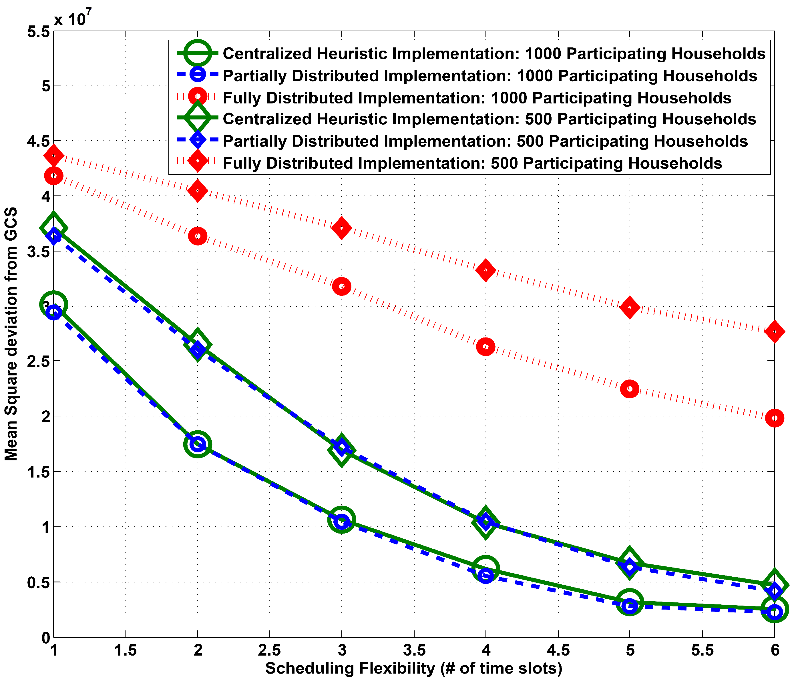
In
Figure 1, we plot the mean square deviation from the GCS
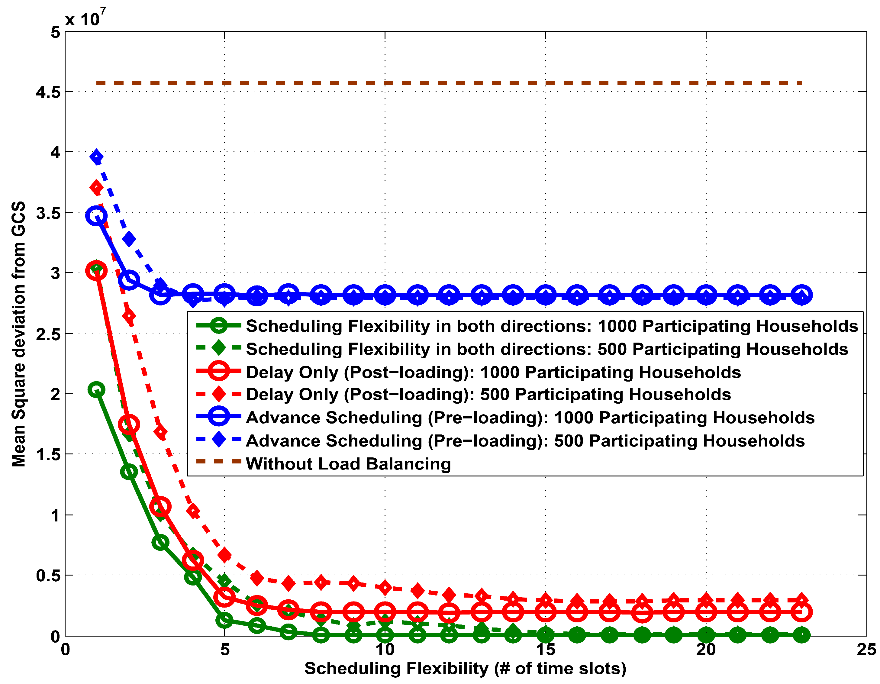
versus scheduling flexibility (in terms of number of time slots) for a centralized heuristic implementation consisting of 1000 households. We consider both 100% and 50% participation rates and we compare the results for different types of scheduling flexibility. We also compare the developed algorithm to a base case, “without load balancing”. This base case represents a traditional grid in which all loads are essential without the ability to reschedule flexible loads. We can observe that just by introducing a small amount of scheduling flexibility of any type can result in a significant increment of demand profile flatness. When flexible loads can be re-scheduled in both directions, the grid has more flexibility and it can achieve a flatter demand profile as compared to both delay only (post-loading) and advance scheduling only (pre-loading) cases.
Figure 1.
Mean square deviation from GCS vs. scheduling flexibility: centralized heuristic implementation with different participation rate of households.
Figure 1.
Mean square deviation from GCS vs. scheduling flexibility: centralized heuristic implementation with different participation rate of households.
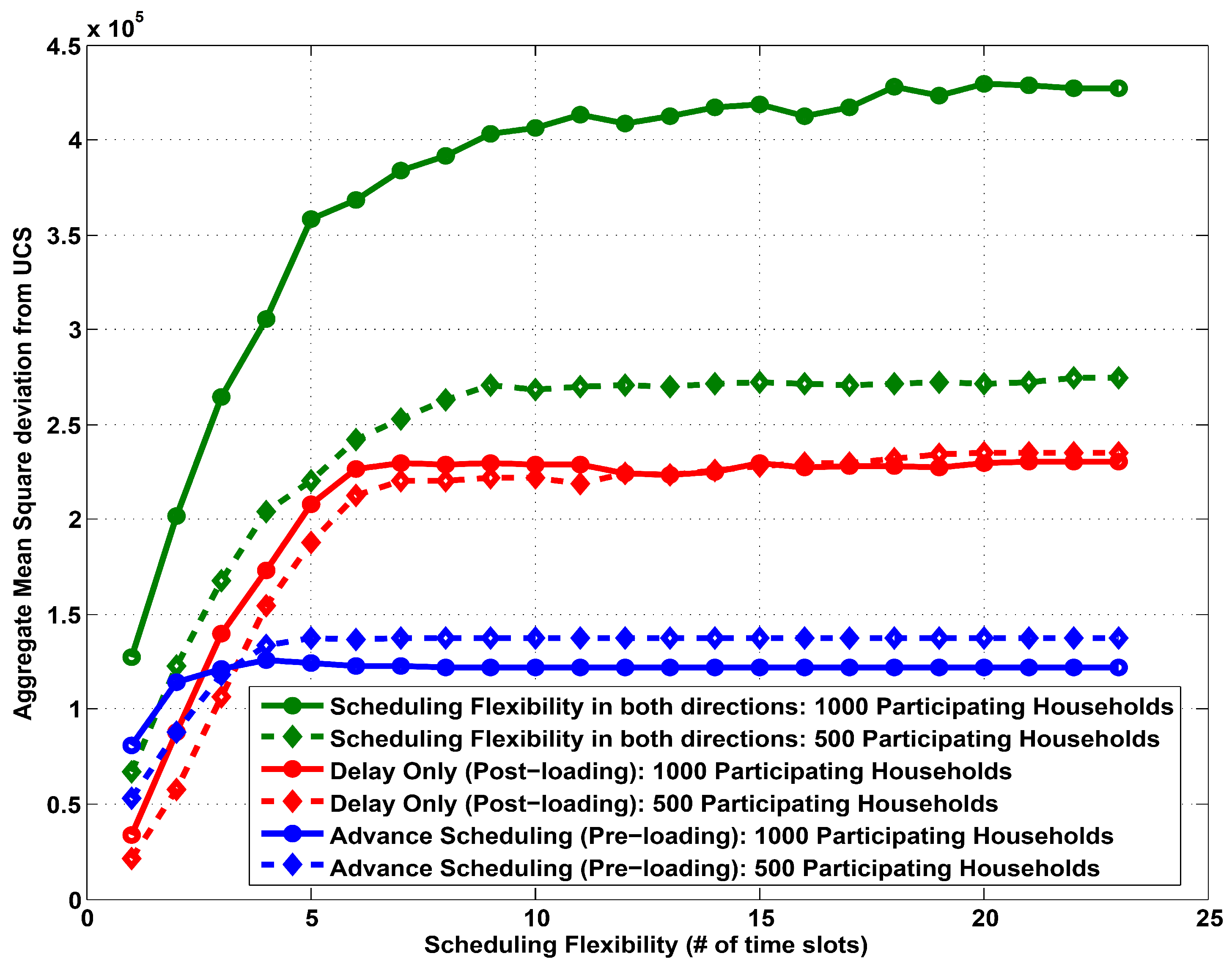
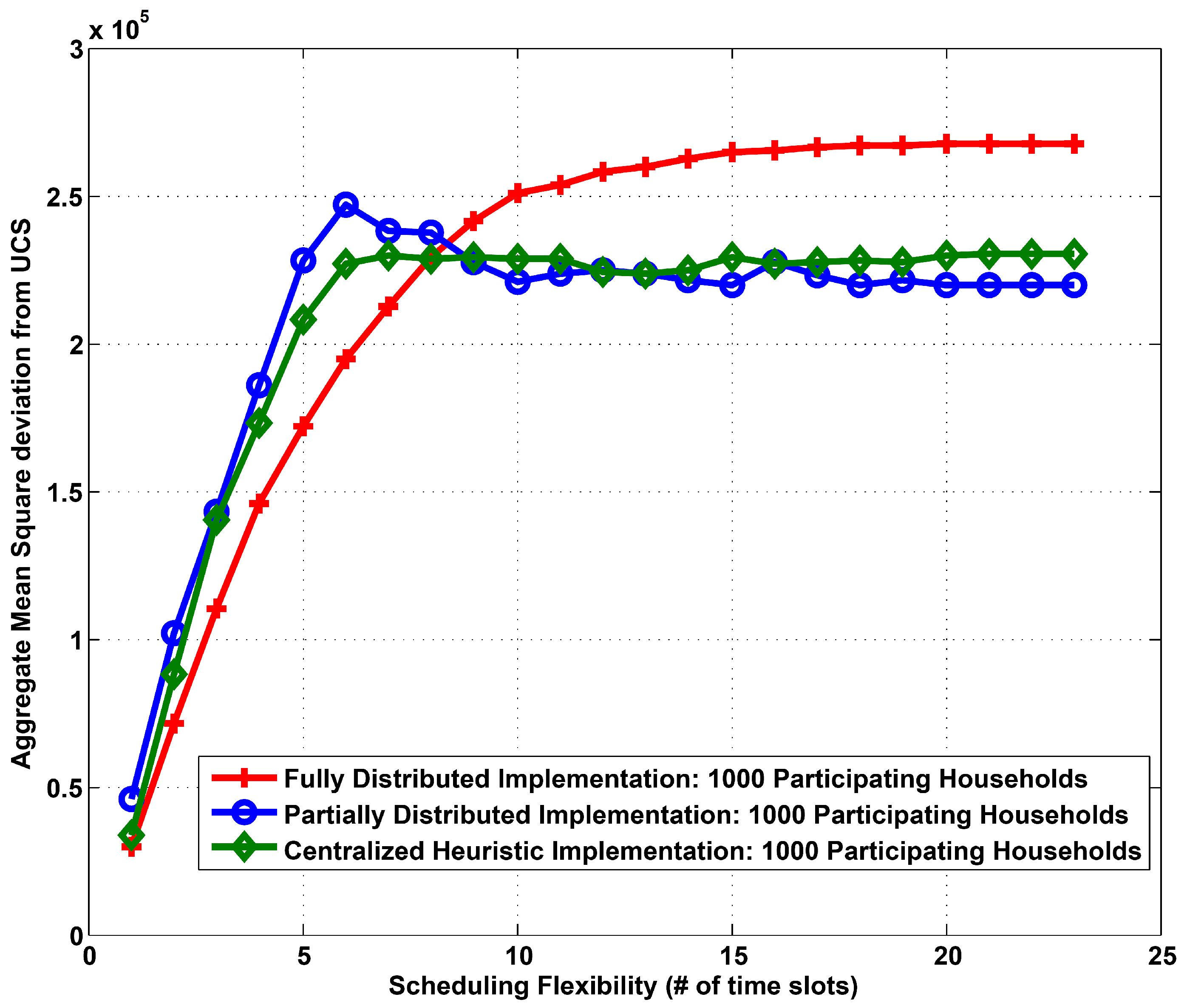
Figure 2 shows the aggregate mean square deviation from UCS against scheduling flexibility for 1000 households adopting a centralized heuristic algorithm.
Figure 2.
Aggregate mean square deviation from UCS vs. scheduling flexibility: centralized heuristic implementation with different participation rate of households.
Figure 2.
Aggregate mean square deviation from UCS vs. scheduling flexibility: centralized heuristic implementation with different participation rate of households.
Again we compare the results for different types of scheduling flexibility and participation rate. We can see that increasing scheduling flexibility in general increases aggregate user inconvenience for all types of scheduling flexibilities. The aggregate user inconvenience is highest when users allow for full flexibility in load scheduling when compared to just restricting scheduling to pre or post loading. This is due to the fact that loads get rescheduled more often in order to achieve the objective of a flatter demand profile. Moreover, it is also obvious that increasing the number of participating households increases the aggregate user inconvenience.
5.2. Comparison of Centralized Heuristic Implementation and Distributed Implementations
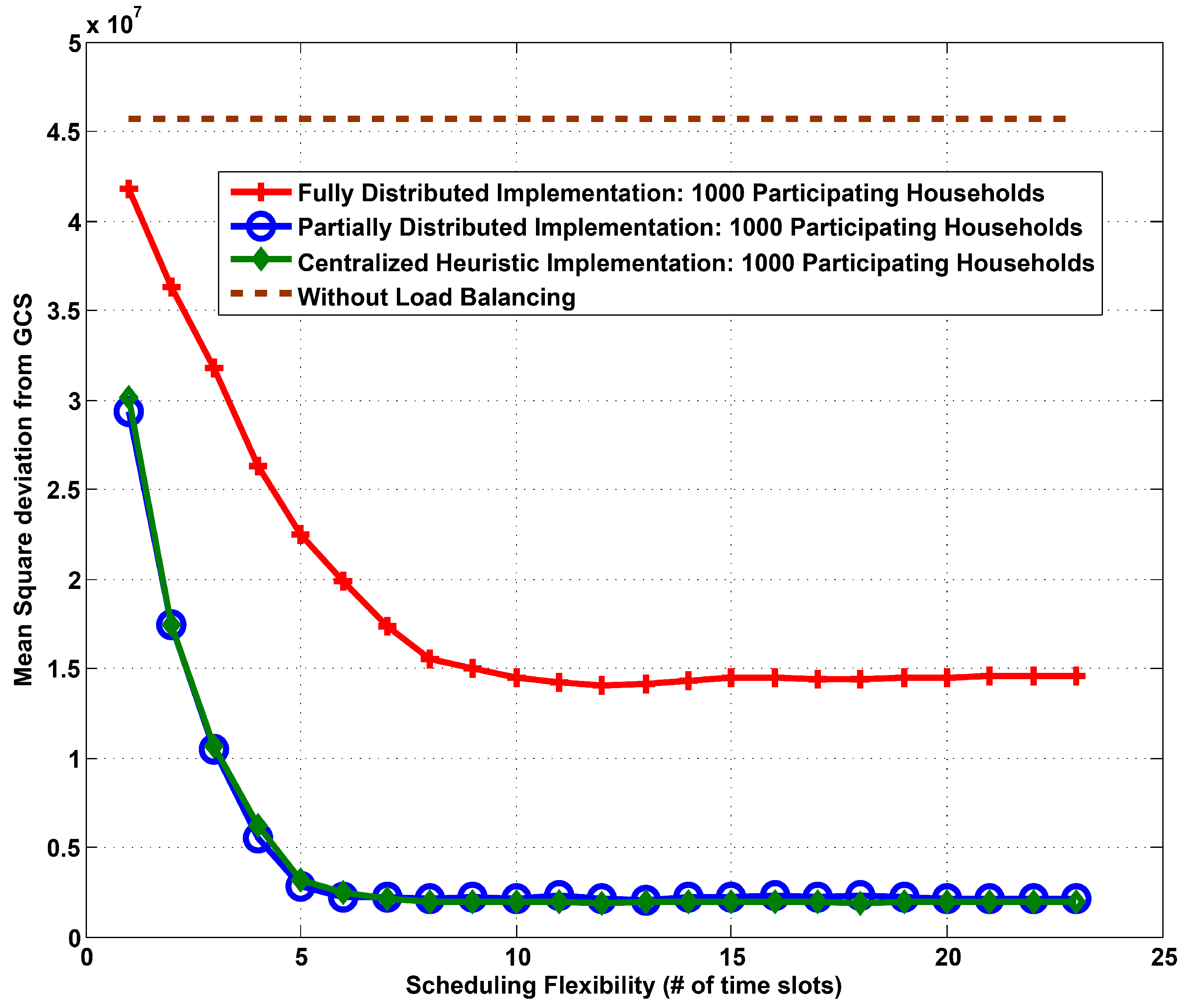
In
Figure 3 and
Figure 4, we compare full and partially distributed implementations to the centralized heuristic implementation. We plot mean square deviation from GCS and aggregate mean square deviation from UCS respectively assuming that all the 1000 households participate. In these simulations, we consider delay only (post-loading) scheduling since the performace is close to full flexibility in scheduling. In
Figure 3, we also compare the developed algorithms with the base case. Again, we see that with just a small level of scheduling flexibility, we can obtain a significant amount of load profile flattening in all implementations. There is a performance gap if there is no coordination between the individual households and a centralized controller. However, the performance of a partially distributed implementation is very similar to a centralized algorithm (Centralized Heuristic). Hence, a probable practical implementation to achieve a flat demand profile could be to allow for distributed scheduling (reduction in data reporting requirement) with a centralized coordinating scheduler.
Figure 3.
Mean square deviation from GCS vs. scheduling flexibility: 1000 participating households.
Figure 3.
Mean square deviation from GCS vs. scheduling flexibility: 1000 participating households.
Figure 4.
Aggregate mean square deviation from UCS vs. scheduling flexibility: 1000 participating households.
Figure 4.
Aggregate mean square deviation from UCS vs. scheduling flexibility: 1000 participating households.
In
Figure 4, we examine user inconvenience against scheduling flexibility for distributed and centralized algorithms. Again increasing scheduling flexibility increases aggregate user inconvenience. We can however observe that the aggregate user inconvenience achieved by the partially distributed algorithm is also comparable to a centralized heuristic implementation, and is much lower than the fully distributed implementation. Considering this result with the previous insight, a partially distributed implementation appears to be the most practical implementation which allows for a flatter demand profile with relatively low user inconvenience.
In
Figure 5 and
Figure 6, we once again compare centralized and distributed implementations, but with a focus on household participation rates. In
Figure 5 we plot the mean square deviation from GCS
vs. scheduling flexibility. We can observe that increasing the participation rate from 50% to 100% results in a flatter demand profile. However, at around a scheduling flexibility of 6 time slots, the demand profile flatness achieved by 500 participating households is almost comparable to the demand profile flatness achieved by 1000 participating households. It suggests that the grid does not require a 100% participation from the households, just requiring a minimum level of household participation in the program. The performance of partially distributed implementation is again seen to be comparable to the centralized heuristic implementation. A similar trend can also be obtained from the looking at the user inconvenience figures for differing participation rates (
Figure 6) .
Figure 5.
Mean square deviation from GCS vs. scheduling flexibility: different participation rate of households.
Figure 5.
Mean square deviation from GCS vs. scheduling flexibility: different participation rate of households.
Figure 6.
Aggregate mean square deviation from UCS vs. scheduling flexibility: different participation rate of households.
Figure 6.
Aggregate mean square deviation from UCS vs. scheduling flexibility: different participation rate of households.
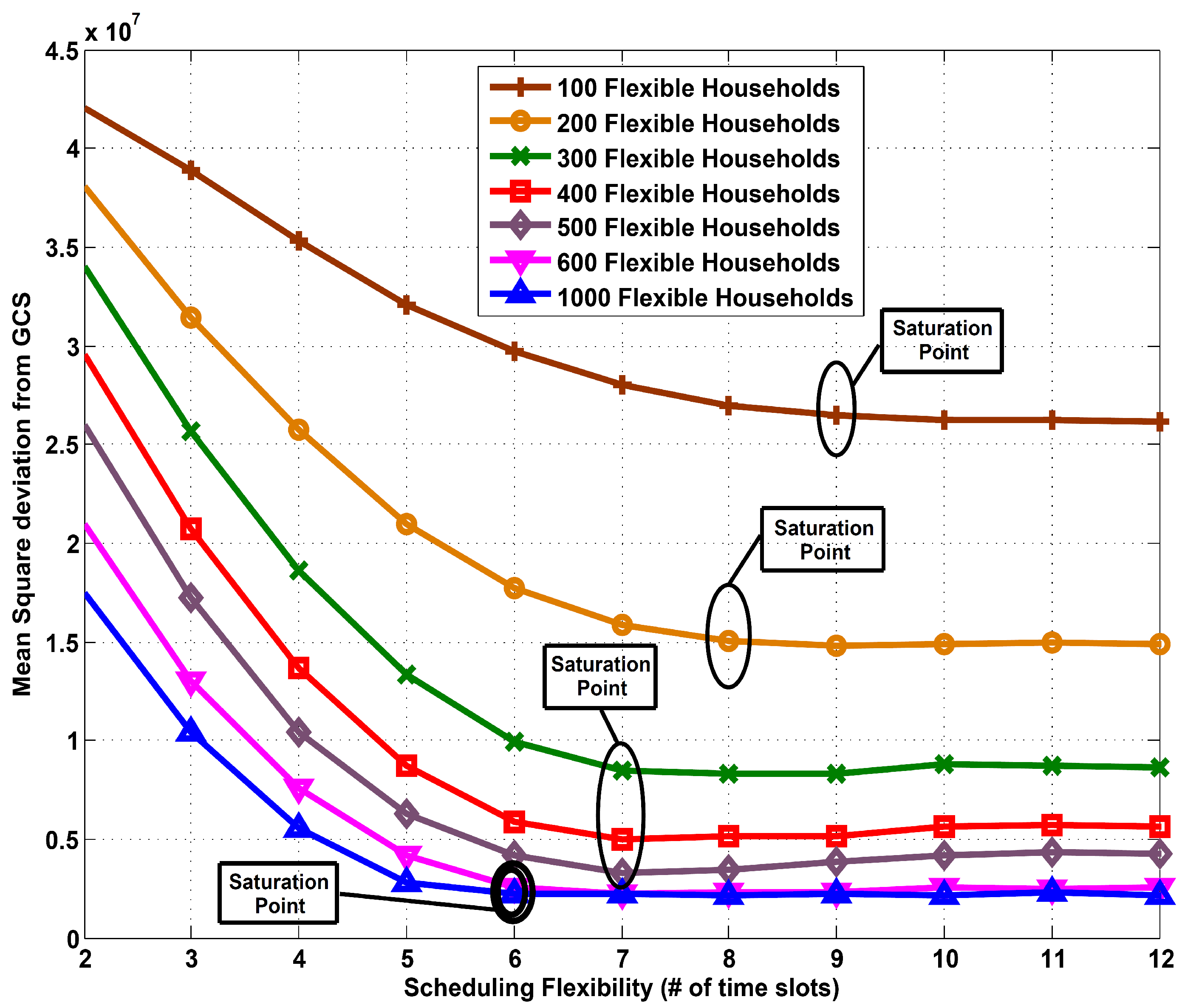
5.3. Existence of a Saturation Point and Impact of User Participation Rate
An important observation from all the above results is the existence of a “saturation point”. For a given user participation rate we define this point as the amount of scheduling flexibility beyond which there are no significant gains in terms of demand profile flatness. In
Figure 3, the saturation point for 1000 participating households for centralized and partially distributed implementations is around 6 time slots. However, to investigate the relationship between participation rate and saturation point we plot
Figure 7. In this graph we plot the participation rate of households
vs. the saturation point for partially distributed implementation. The saturation point is also marked on the graph. We can see that when the user participation increases from 100 to 600 households, saturation point shifts from 9 time slots to 6 time slots. However, the saturation point remains unchanged when the participation rate is further increased for the simulated load model. The saturation point cannot be further decreased even if all the households participate. Thus for any user participation rate, the grid always requires a certain amount of scheduling flexibility in loads to achieve demand profile flatness.
Figure 7.
Participation rate of households vs. saturation point: partially distributed implementation.
Figure 7.
Participation rate of households vs. saturation point: partially distributed implementation.
6. Conclusions
In this paper we studied the impact of scheduling flexibility on demand profile flatness and user inconvenience in a residential smart grid system. We considered three type of scheduling flexibility (delay only, advance scheduling only, and fully flexible) in flexible loads. The optimization problem proved to be NP-hard. We developed optimal and sub-optimal scheduling algorithms and discussed their centralized and distributed implementations. The distributed implementation offers households better privacy protection through the reduction of information sharing with a centralized scheduler.
However, a fully distributed system performs significantly worse than a centralized implementation. Hence, we also propose a partially distributed implementation, where a grid coordinates among all the users. Such a system approaches the performance of a centralized system. We also identified the existence of a saturation point, where for a certain user participation rate, a point exists where increasing scheduling flexibility beyond this point hardly affects the demand profile flatness. Thus the limitation of scheduling flexibility to only few time slots could be is beneficial to both the grid as well as to the users. Furthermore, the grid also does not require participation from all the households, and it can achieve a relatively flat demand profile by encouraging a minimum level of user participation.
7. Discussion and Future Work
In this paper we developed a framework to study the impact of scheduling variations on demand profile flatness and user inconvenience. We developed algorithms to study the compromise or trade-off points between gird inconvenience and user inconvenience in the form of saturation point and minimum user participation rate. We modeled TCLs as fixed power consumption loads. However, it would be interesting to consider more detailed thermal dynamic models for TCLs which can capture the turn-on time and TCL duration correlations in different time slots. New metrics will be required to measure the impact of these correlations (according to the underlying thermal dynamic model for TCL) on user comfort and demand profile flatness. Additionally operational constraints of TCLs can also be considered. Thus with additional constraints and a more detailed load modeling, several other parameters such as switching frequency of TCLs (which has an impact on the lifetime of TCL), total power consumption, peak power reduction, etc. will also come into focus. Such formulation and modeling therefore can also be useful to optimize additional parameters. In fact a multi-objective optimization problem could be formulated by giving different weights to different parameters. For example, one may give more weight to the reduction of TCL switching frequency compared to peak reduction or more weight can be given to total power consumption reduction, etc. Again in such formulations, how different weights affect demand profile flatness and user inconvenience have to be investigated.
The framework developed in this paper could still be used if more complicated load models or weighted multi-objective problems are considered. However, new metrics to measure demand profile flatness and user inconvenience according to the underlying thermal dynamic TCL models, or weighted objectives will be required. Moreover, new algorithms have to be developed to accommodate the additional operational constraints and objectives in the optimization problem. These considerations will have an impact on the saturation point and minimum user participation rate and will be worth investigating. Finally designing proper incentives based on the saturation point and minimum user participation rate will also be investigated in future.

