1. Introduction
The modern power system is experiencing an unprecedented evolution. On the one hand, large-scale interconnected power systems have emerged in some countries. On the other hand, the installed renewable energy capacity, especially the wind power, has been increasing rapidly to satisfy the growing power demand and the desire for sustainable development.
With the interconnection of large regional grids, tie-line power oscillations happen more frequently than before, which can limit the transmission capacity or even jeopardize the system stability. For instance, in Finland-Sweden-Norway-Denmark system and Western Electric Coordinating Council system (WECC), tie-line power oscillations have resulted in the separation of the interconnected system on some occasions [
1]. Normally, tie-line power oscillations are associated with inter-area oscillations which involve two coherent groups of generators swinging against each other. This type of oscillation corresponds to a low frequency oscillation which frequency is in the range of 0.1–2.5 Hz [
2].
Previous work has pointed out that cyclic external disturbances can result in a significant response in power systems, when their fundamental frequency is close to the low-frequency oscillation mode (including inter-area mode) of the system [
3,
4]. These kinds of oscillations are termed forced oscillations. In the past, the forced oscillations didn’t arouse much attention, as they showed little impact on power system stability. However, in recent years, forced oscillation accidents induced by small hydro plants have happened several times in the China Southern Power Grid, which is a typical interconnected grid with low damping inter-area modes [
5]. Hence, attention to forced oscillations has been renewed.
Wind power variations can also be considered as an external disturbance to power systems. Power variations produced by wind turbines during continuous operation are mainly caused by wind speed variations, tower shadow effects, wind shear effects,
etc. The effects of tower shadow and wind shear (TSWS) produce a periodic reduction in mechanical torque at a frequency called the 3p frequency [
6]. The 3p frequency range, due to rotational sampling as each blade passes the tower, tends to coincide with the frequency range associated with inter-area oscillations, so the power variations induced by TSWS might be a source of forced oscillations that can excite system resonance.
The TSWS are referred to as 3p oscillations. The 3p oscillations once aroused great attention from the power quality point of view, as researchers have found that 3p oscillations are one of the main contributors to flicker emissions produced by wind farms. Compared with fixed-speed wind turbines, variable-speed wind turbines have shown better performance in flicker emission [
7]. Subsequently, several active or reactive power control methods have been proposed to eliminate flicker, especially for variable-speed wind farms [
7,
8,
9]. However, the effects of power variations due to TSWS are not taken into account in the assessments of power system stability assuming that the mechanical torque for the wind turbine is constant [
10]. That is to say, comprehensive understanding of the adverse effects of 3p oscillation is still limited, and it is necessary to reevaluate this phenomenon.
Recently, the power system oscillations induced by TSWS have been discussed. Brownlees
et al. [
11] have investigated the impact of TSWS from fixed-speed wind farm power oscillations on the Irish Power System based on recorded data analysis. Hu
et al. [
12] have simulated that the TSWS of a wind farm can induce tie-line power oscillations. However, the above results are preliminary and cannot readily offer qualitative conclusions, so the underlying mechanism needs to be studied further. Besides, it is also important to quantify the magnitude of tie-line power oscillations induced by 3p oscillations and to study the qualitative effects of parameters.
With the aim of evaluating the impact of TSWS on tie-line power oscillations, this paper addresses the issue of integration of a large-scale wind farm into interconnected power systems. In
Section 2,
Section 3,
Section 4, the transfer functions of a wind farm, a simplified two-zone system and a combined system are developed, respectively. Frequency domain analysis is used to identify potentially amplified-response conditions, the worst case and qualitative parametric effects. In
Section 5 and
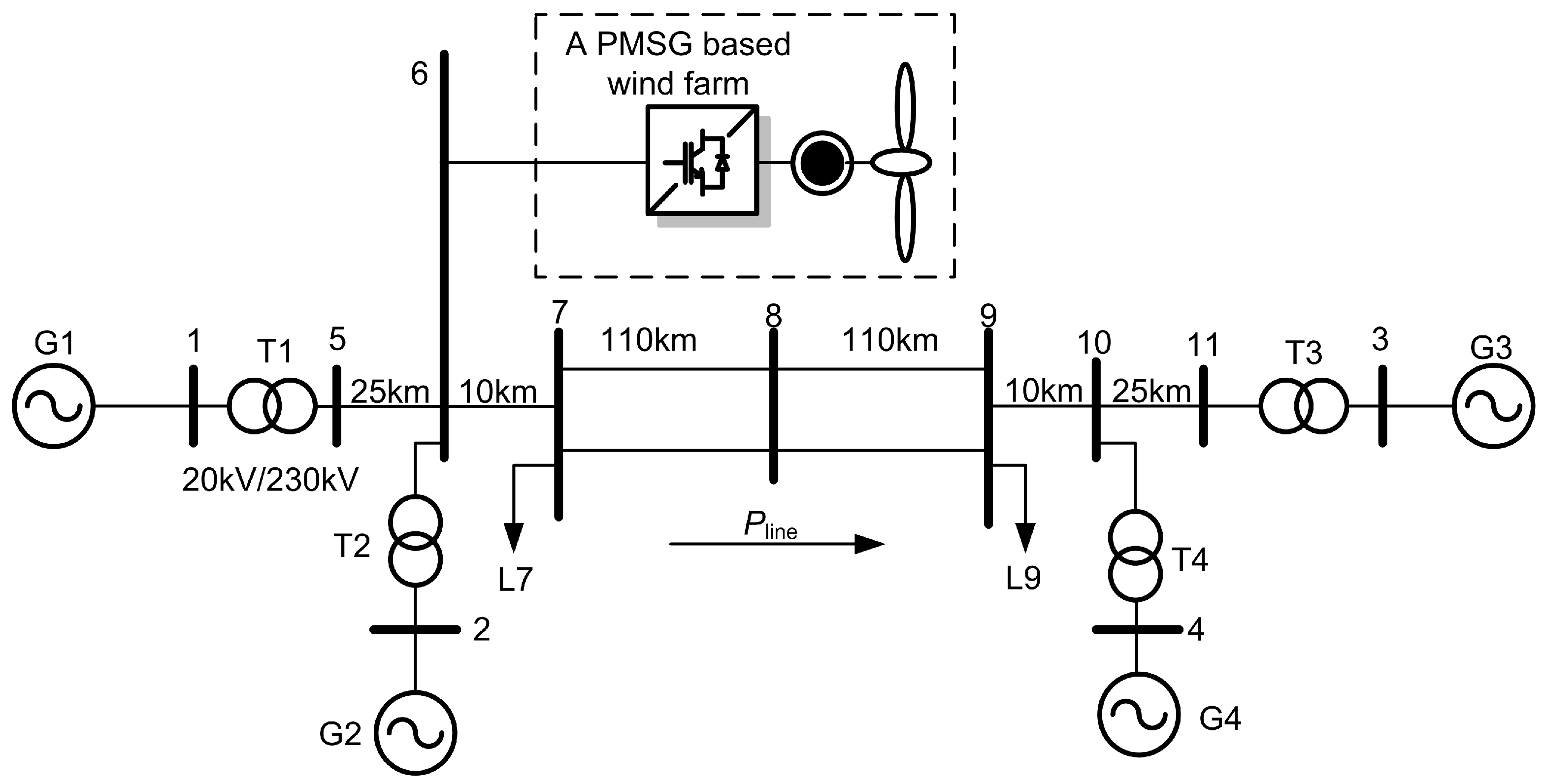
Section 6, time-domain simulations are subsequently applied in the two-area four-generator test system and the more realistic WECC 127 bus system to accurately quantify the effect in the worst case. A new horizon is provided to see how and when the TSWS affect power systems stability.
2. Disturbance Source Modeling
Wind turbine models for power system studies have been widely discussed. The fixed-speed wind turbine models mainly include the aerodynamics model, the shaft model, the generator model and pitch control. With the development of wind turbines, the technology has switched from fixed to variable speed. The variable-speed wind turbine models include more models like the converters model and their controller model.
Since the phenomenon of inter-area oscillations is the topic of interest, a simplified wind turbine and system models in the frequency domain are proposed, which only consider the dynamic model in the low frequency oscillations range. However, the complete models of the wind turbine and power systems are adopted in the simulation study to verify the results.
2.1. Aerodynamics Model
Because the electrical behavior of wind turbines is the main topic of interest of the study, a simplified aerodynamic model [
13] is used as follows:
where
Tm is the mechanical torque,
ρ is the air density,
R is the wind turbine rotor radius,
Veq is the equivalent wind speed,
Cp is the aerodynamic efficiency of rotor,
λ is the tip speed ratio and
θ is the pitch angle of the rotor.
Most studies concerning the stability of power systems with integrated wind power generally neglect the 3p oscillations. Here, a comprehensive model of 3p mechanical torque for a three-blade wind turbine [
6] is adopted. Based on this model, the equivalent wind speed can be expressed by three components, as follows:
where
VH is the wind speed at hub height,
Veqws is the wind shear component,
Veqts is the tower shadow component. The latter two components can be represented as:
where
α is the empirical wind shear exponent,
H is the elevation of rotor hub (m),
β is the azimuthal angle of the blade (deg),
βb is the azimuthal angle of each blade (deg),
a is the tower radius (m),
x is the distance from the blade origin to the tower midline (m), and
m = 1 + [
α(
α− 1)]/8 × (
R/
H)
2 is a coefficient of the wind turbine.
Linearizing Equation (1) and substituting for Veq given by Equation (2), it indicates that mechanical torque variations induced by TSWS are also periodic and the magnitude of 3p oscillations varies with different mechanical and operation parameters of wind turbines.
The 3p frequency (
f3p) is three times of rotor frequency. For different fixed-speed wind turbines, typically,
f3p can be in the range of 0.65 Hz to 1.5 Hz, which is calculated from some typical parameters provided by Siemens and Vestas (Aarhus, Denmark) [
11,
13], and the magnitude of 3p oscillations power is about 10% of the average power output.
For a variable-speed wind turbine, the
f3p of the popular variable-speed wind turbines varies from 0.25 to 0.9 Hz which is calculated from some typical parameters provided by General Electric Co. (GE, Fairfield, CT, USA) and Siemens Wind Power A/S (Brande, Denmark) [
13,
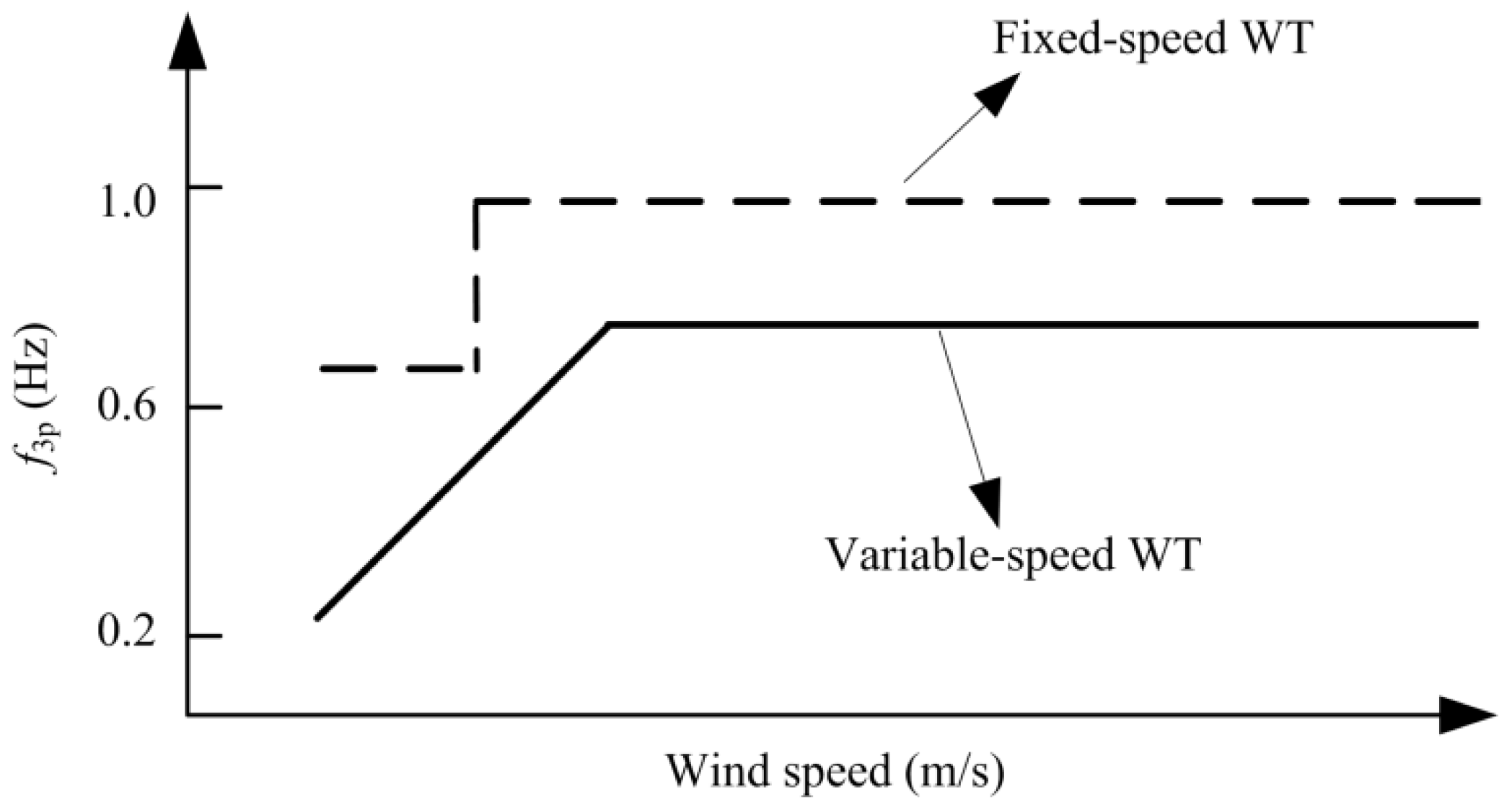
14]. Taking a GE 2.7 MW variable-speed wind turbine and Siemens 1.3 MW fixed-speed wind turbine as examples, we plot the 3p frequency under different wind speeds, as shown in
Figure 1.
Figure 1.
3p Frequency with two types of wind turbine.
Figure 1.
3p Frequency with two types of wind turbine.
Figure 1 shows that the
f3p is in the range of interest of low frequency oscillations. This fixed-speed wind turbine has two 3p frequencies for a switch between the two windings and it is easy to form a sustainable oscillations source. When a variable-speed wind turbine operates at its maximum power point tracking (MPPT) range, the
f3p is proportional to the wind speed, while the wind speed is above the rated wind speed, the
f3p is constant. When the variable-speed wind turbine operates around a fixed wind speed or at mid-high wind speed, the variable-speed wind turbine can also form a forced oscillations source.
2.2. Shaft Model
The wind turbine system has a low resonant frequency due to the softness of the low speed shaft. Thus the dynamics of the shaft model need to be taken into account. The two-mass model representation of the shaft is proper to illustrate the dynamic impact of wind turbines on low frequency oscillations in grids. The linearized form of the shaft two-mass model [
13] is:
where
Pe is the electric power of the generator,
Pm is the mechanical power produced by rotating wind turbine,
ω1,
ω2 are the speeds of the wind turbine and the generator rotor,
ω0 is the rated grid speed,
θ is the twist angle in the shaft system,
K12 is the shaft stiffness,
D12 is the damping coefficient between wind turbine and generator,
HW and
HG are inertia constants of the wind turbine and generator, the prefix Δ denotes a small deviation.
By taking the Laplace transform of Equation (5), the equations can be written in the frequency domain with the initial conditions of state variable deviations assumed to be zero as:
Since the wind turbine is operating in the speed control mode, Δ
ω2 can be assumed to be zero. The response of electrical power can be derived from Equation (6), as follows:
2.3. Generator Model, Converter Model and Control Strategies
For convenience, a variable-speed wind turbine based on a multi-pole permanent magnet synchronous generator (PMSG) [
15] is applied here as an example. We should note that in this study the PMSG only adopts basic control without ancillary controllers to eliminate the 3p oscillations. Neglecting the stator transient, the equations of a PMSG can be expressed by a set of algebraic equations [
2].
For the converters, the switch frequency of the power electronic components far exceeds the frequency band of interest, so an average model is used without considering switch dynamics [
16].
Normally, variable-speed wind turbines have two control goals, depending on the wind speed. At low-moderate wind speeds, the rotor speed can be adjusted with the wind speed so that the optimal tip speed ratio is maintained for maximum power point tracking (speed control mode). At high wind speeds, the wind turbine maintains the rated output power by adjusting the pitch angle and keeping the rotor speed constant (power limitation mode). The vector-control is used to realize the decoupled control of active power and reactive power. The control strategies used in this study are based on the idea [
15] that the generator-side converter controls the rotor speed to maintain the optimal tip speed ratio and minimize the power losses in the generator, while the grid-side converter control DC-link voltage constant and reactive power flow to the grid. More details on the controller model are given by Chinchilla
et al. [
15]. In the time scale of electromechanical dynamic, the power loss of power electronic converter can be ignored. Hence, the output power fluctuation of a wind turbine Δ
PWT approximately equals to Δ
Pe.
2.4. Wind Farm Model
The fluctuation power of a wind farm which consists of
N wind turbines can be expressed as:
where
α1 is the TSWS weaken factor (0 <
α1 < 1),
i is the number of wind turbines, and Δ
PmN is the sum of the mechanical power fluctuation of
N wind turbines.
Normally, for every wind turbine in a wind farm, the time of a blade passing by the tower is stochastic. The power drop time depends on not only the rotor speed, but also the initial phase. This means that a wind farm’s power fluctuation induced by TSWS will be weakened due to the random blade position. When
α1 = 0, it represents that the TSWS can be totally cancelled out if the turbines could be controlled to distribute the rotor angle evenly. When
α1 = 1, it represents that the blades are synchronized and the blades are passing by the tower at the same time, thus the superposition of the 3p oscillations will cause the maximum power fluctuation (
NΔP
WT). It should be noted that, the case of
α1 = 1 is not expected to represent a typical operation but rather to be a representative of “the worst case”. Since we try to figure out the worst impact of the TSWS on power systems, we choose the case of
α1 = 1 for the following study. With per unit expression, Δ
PmN = Δ
Pm, then the transfer function representing the relationship between mechanical power fluctuation and output power fluctuation of the wind farm can be expressed as:
According to Equation (9), the frequency characteristic of the wind turbine system shows that the wind turbine acts like a low pass filter and when the mechanical power disturbance is constant, the wind power variation of a wind farm is linear to the TSWS weaken factor
α1. Based on some typical parameters of a wind turbine [
13], the natural resonant frequency of the wind turbine (
f1n) is in the range of 0.11 to 0.82 Hz which means that the 3p oscillations are likely to be amplified in the wind turbine. Besides, it is notable that the operation point of the wind turbine has no effect on its natural frequency.
3. Tie-Line Power Oscillations Induced by a Wind Farm
3.1. Modeling of Tie-Line Power Oscillations
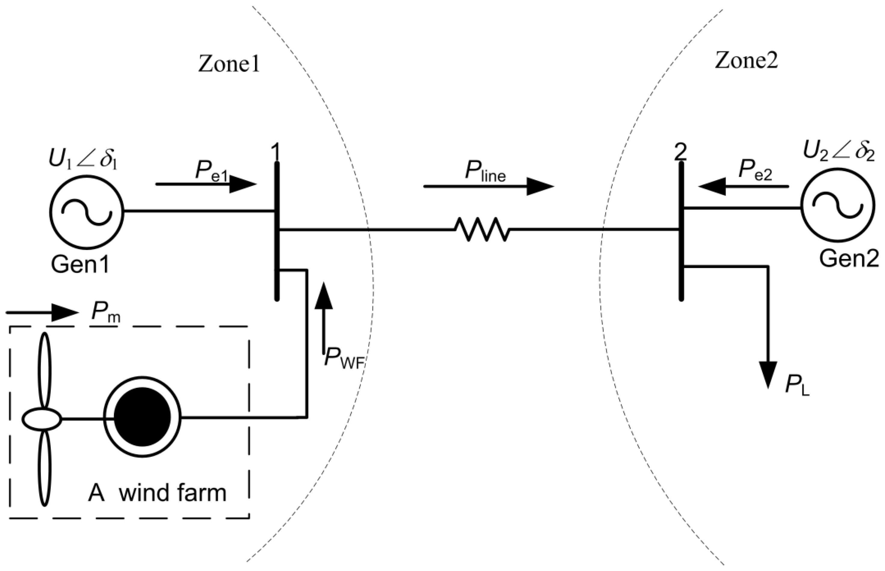
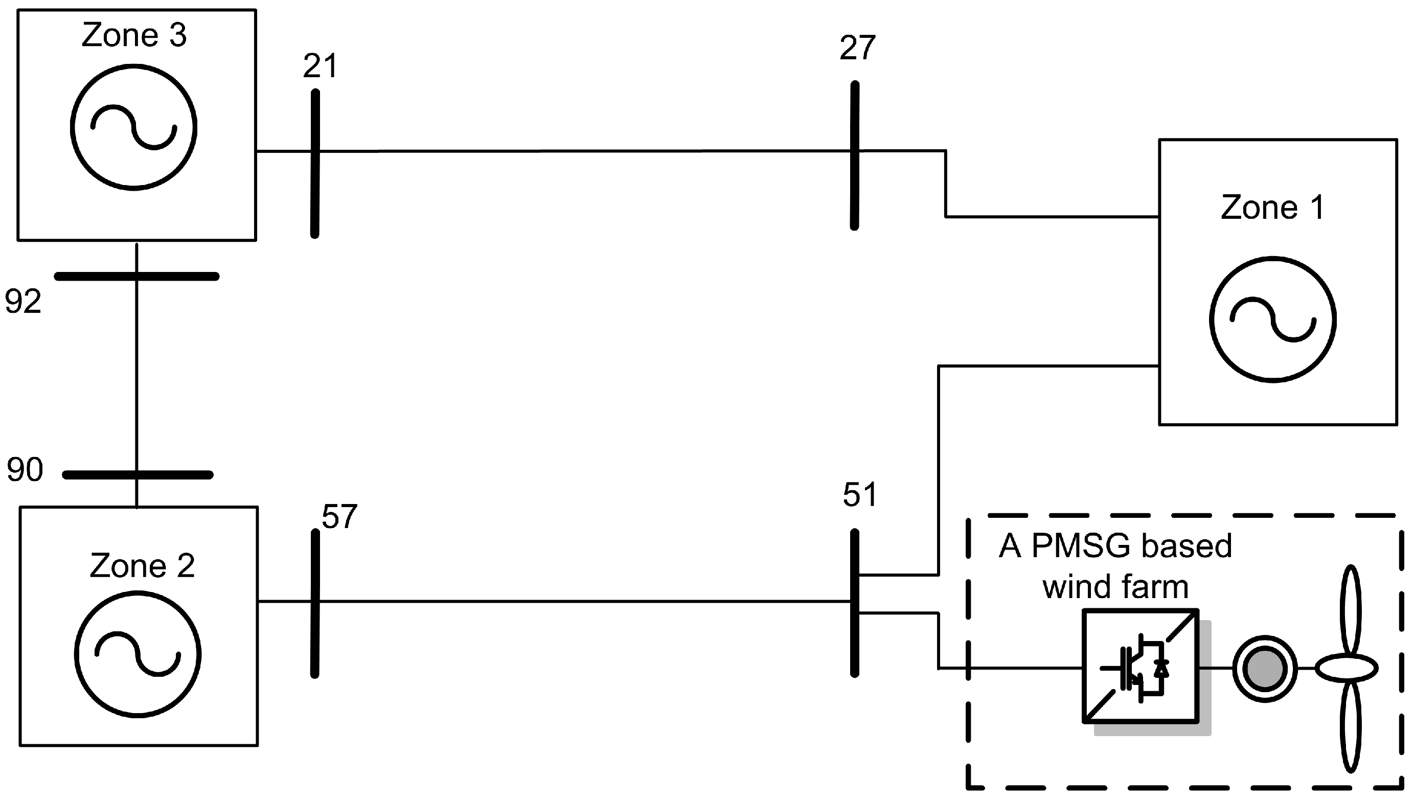
For a typical two-area interconnected power system, the closely coupled generators in each zone can be equivalent to one generator. Therefore, in order to focus on how power variations of a wind farm affect the tie-line power, a simple two-machine system with a wind farm is constructed. The configuration is shown in
Figure 2. The system consists of two similar generators (Gen 1 and Gen 2) and a wind turbine which is connected to Bus 1. Analysis of a system with such a simple configuration is useful in understanding the fundamental of tie-line power oscillations and studying the parametric effects.
Figure 2.
A two-machine system with a wind farm.
Figure 2.
A two-machine system with a wind farm.
With the synchronous generator represented by a classical model [
2], the linearized swing equations of Gen1 and Gen2 are given by:
where
H1,
H2,
δ1,
δ2,
KD1,
KD2 are the inertia constants, the rotor angles, the damping coefficients of Gen1 and Gen2, respectively;
Pm1,
Pm2,
Pe1,
Pe2 are the mechanical power and the electrical power of Gen1 and Gen2.
According to the power conservation principle with assuming the tie-line is lossless, we obtain:
where
PWF,
Pline,
PL are the active power of the wind farm, the tie-line and the load.
Here Δ
Pline can be expressed as:
where
x12 is the reactance of the tie-line,
δ120 and Δ
δ12 are the initial angle difference and the angle difference deviation between Gen1 and Gen 2.
U1 and
U2 are the terminal voltages.
Assuming that Δ
Pm1 = Δ
Pm2 = 0, Δ
PL = 0, for convenience, the model adopts equivalent damping [
17], by defining
KD1/2H1 = KD2/2
H2 = KD. Combining Equation (11) with Equation (10) and substituting for Δ
δ12 by Equation (12) and we have:
where
![Energies 06 06352 i013]()
.
By defining
![Energies 06 06352 i014]()
, which can be treated as the contribution factor of the wind farm power variations, and taking the Laplace transform of Equation (13), the transfer function representing the relationship between the wind farm power variations and the tie-line power oscillations can be expressed as:
According to Equation (14), the frequency response characteristic is not only dependent on the system parameters, but also the initial operation point which is associated with δ120, U1 and U2. In general, system natural frequency (f2n) is in the low frequency oscillation range of 0.1 to 2.5 Hz in interconnected systems.
3.2. Frequency Response Analysis
Frequency response characteristic illustrates the severity of the disturbance under different frequencies. A numerical example based on typical parameters [
2] is used to demonstrate the tie-line frequency response characteristic. The values of the system parameters are as follows:
H1 = 6.5 s,
H2 = 6.175 s,
KD1 = 5,
U1 = U2 = 1.01 p.u.,
δ120 = 0.4 rad,
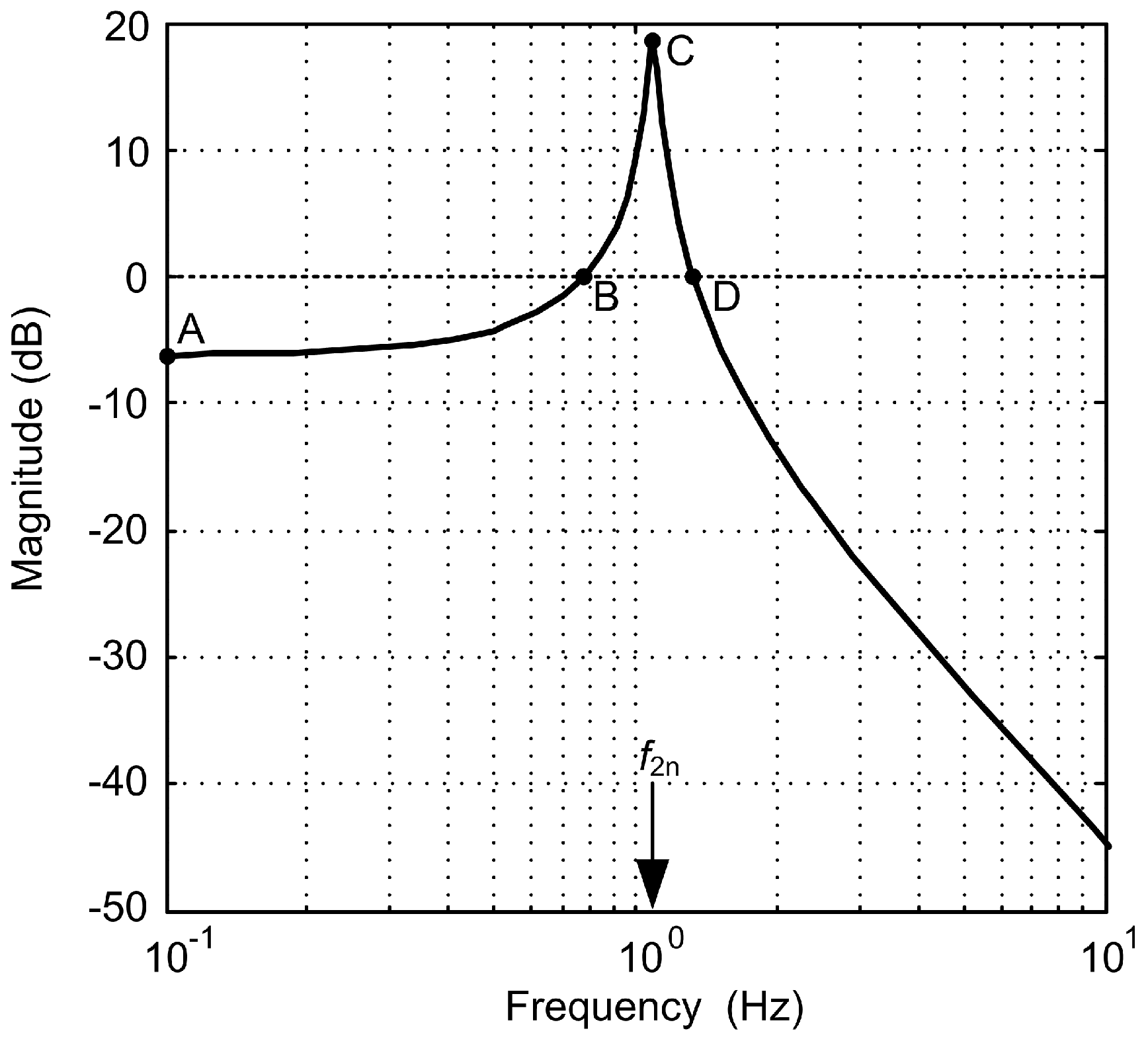
x12 = 1 p.u. Based on above parameters, the amplitude-frequency response characteristic of
G2(j
ω) is plotted in
Figure 3.
Figure 3.
Amplitude-frequency response characteristic of G2(jω).
Figure 3.
Amplitude-frequency response characteristic of G2(jω).
When f3p ∈ [A,B], |G2(jω)| < 1. Namely, the tie-line power oscillation is less than the power fluctuation of a wind farm (A: |G2(jω)| = 0.51, B: |G2(jω)| = 1), which means that the synchronous generators dampen the disturbance of the wind farm in AB. When f3p ∈ [D,∞), |G2(jω)| < 1 and attenuates very fast, which means that the two-machine system acts as a low-pass filter and thus the high-frequency disturbance from a wind farm has little effect on the tie-line power (D: |G2(jω)| = 1). When f3p ∈ (B,D), |G2(jω)| ≥ 1. Namely, the amplitude of the tie-line power oscillation is larger than the power fluctuation of a wind farm. Especially, when f3p closes to the system natural frequency f2n (C: |G2(jω)|max = 8.71, f2n = 1.09 Hz), the tie-line power oscillations will be sharply amplified, which is caused by resonance.
3.3. The Expression of the Peak Magnitude
The occurrence of resonance is a severe disturbance to power systems. Therefore, it is essential to evaluate the peak magnitude of the tie-line power resonance. Define the damping ratio
![Energies 06 06352 i016]()
and let
ω2n = 2π
f2n =
![Energies 06 06352 i017]()
, thus
G2(
s) can be rewritten as a standard form as follows:
Let the derivative of Equation (15) with respect to
ω/
ω2n equal to be zero and the expression of the system resonant frequency
ωr is:
Normally, the typical damping ratio of inter-area mode in power systems is close to zero [
2], so
ωr is close to
ω2n according to Equation (16). Consequently, when
f3p approaches the system natural frequency
f2n, the resonant peak magnitude of the tie-line power oscillations is given by:
3.4. Parametric Analysis
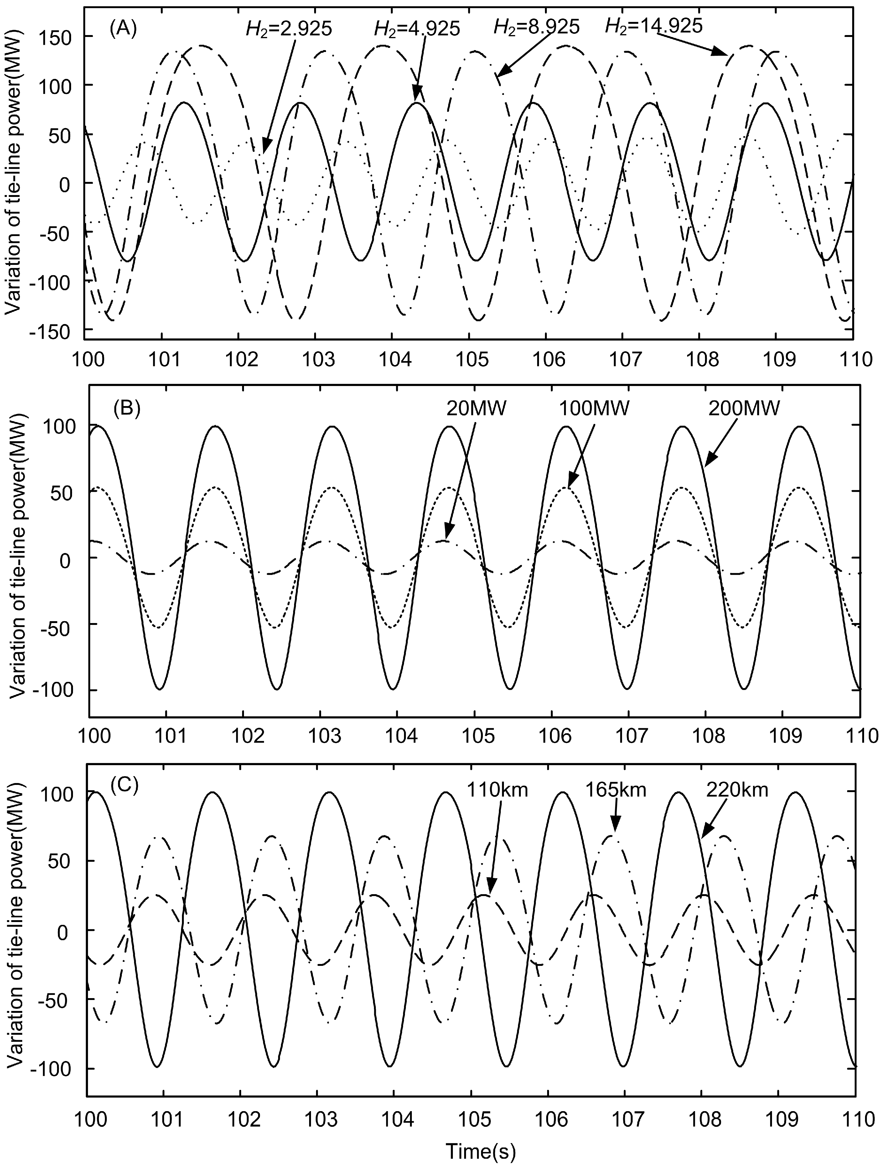
Equation (17) illustrates that the resonant magnitude of the tie-line power oscillation is dependent on three factors: the disturbance magnitude of the wind farm (ΔPWF), the inertia constant ratio of two-area systems (H1/H2) and the system damping ratio (ζ). As ΔPWF increases, or H1/H2 deceases, or ζ decreases, the peak magnitude of the tie-line power oscillations increases. H1/H2 > 1 means that the wind farm connects to a relatively big grid, H1/H2 < 1 means that the wind farm connects to a relatively small grid and H1 = H2 means that the wind farm connects to a grid with two identical areas.
As shown in
Table 1, the numerical examples are given to calculate
|G2(j
ω)
|max with three different inertia constant ratios,
i.e., 1/25, 1/1, and 25/1, denoted by Case 1 Case2 and Case3. In each case, there are three damping ratios,
i.e., 0.3, 0.05 and 0.01, corresponding to the good, medium and poor damping, respectively.
Table 1.
|G2(jω)|max with different inertia constant ratios and damping ratios.
Table 1.
|G2(jω)|max with different inertia constant ratios and damping ratios.
| Case | H1/H2 | |G2(jω)|max |
|---|
| ζ = 0.3 | ζ = 0.05 | ζ = 0.01 |
|---|
| 1 | 1/25 | 1.60 | 9.62 | 48.08 |
| 2 | 1/1 | 0.83 | 5 | 25 |
| 3 | 25/1 | 0.06 | 0.38 | 1.92 |
Table 1 shows that with “big” grid connections (e.g., Case 3) the wind farm has limited influence on the tie-line power fluctuations. When the resonance happens in a medium damping system (ζ = 0.05), the tie-line power oscillations induced by TSWS can be neglected since |Δ
Pline| is less than half of |Δ
PWF|.
However, when the wind farm is integrated into a “small” grid (e.g., Case 1), even with a good damping system (ζ = 0.3), |ΔPline| is 1.6 times higher than |ΔPWF|. Furthermore, with a poor damping of the tie-line mode, |ΔPline| is 48.08 times higher than |ΔPWF|. Thus attention must be paid to the risk of the tie-line power oscillations.
In some countries, such as China, the wind sources may be far away from the load centers. Because it is hard to accommodate all the wind power in the local grid, the residual wind power has to be transferred to a distant load center through long transmission lines, e.g., the wind power in Gansu Jiuquan is a practical case [
18]. This is similar with Case1. Thus the risk of the tie-line power oscillations induced by TSWS is worthy of discussion.
4. Combination of the Wind Turbine System and Power Systems
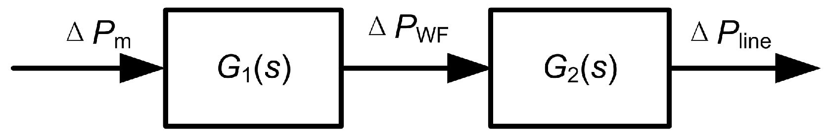
According to
Figure 2, the tie-line power oscillations induced by 3p oscillations can be described by the form of two subsystems series in
Figure 4. The overall frequency response of the cascade of two subsystems is the product of the individual frequency response.
Figure 4.
Block diagram of the series interconnection of the two subsystems.
Figure 4.
Block diagram of the series interconnection of the two subsystems.
Combining Equation (9) with Equation (14), the transfer function of representing the relationship between Δ
Pm and Δ
Pline can be expressed as:
For analyzing the combined impact of these two subsystems, two sets of typical parameters are used in the following example. For the wind turbine system,
Hw = 4.54 s,
K12 = 0.5 p.u./el.rad,
D12 = 7.5 p.u./el.rad. For the two-machine system, the values of the parameters are the same as those in
Section 3.2. For power systems,
G1(s) is normally fixed due to the unchangeable mechanical characteristics of the wind turbine, whereas
G2(s) continuously changes with different system operation conditions or power flows.
The amplitude-frequency characteristics of
G1(j
ω),
G2(j
ω) and
G3(j
ω) are calculated based on the aforementioned parameters, as shown in
Figure 5, where the two panels correspond to two different cases: (A)
G1(j
ω) and
G2(j
ω) have different natural frequencies,
i.e.,
f1n ≠
f2n, (B)
G1(j
ω) and
G2(j
ω) have equal natural frequencies,
i.e.,
f1n ≈
f2n.
Figures 5A,B has same
G1(j
ω), but different
G2(j
ω) by changing the reactance of the tie-line. In the plots, each peak is an indication of a resonant frequency in systems. A relatively large response can be achieved, when
f3p approaches the resonant frequency (
f1n or
f2n).
Figure 5.
Amplitude-frequency characteristic of G1(s), G2(s) and G3(s). (A) f1n ≠ f2n; (B) f1n ≈ f2n.
Figure 5.
Amplitude-frequency characteristic of G1(s), G2(s) and G3(s). (A) f1n ≠ f2n; (B) f1n ≈ f2n.
Figure 5A illustrates that when the wind turbine systems are integrated into a two-machine system, another new peak is created in the low frequency range (
f1n = 0.66 Hz), which was not reported in previous studies. Because the natural frequency of the soft shaft of the wind turbine is within the low frequency oscillation range and thus it may be able to interact with the electromechanical performance of power systems. The plot of |
G3(j
ω)| shows that the amplified frequency range is from 0.44 to 1.21 Hz (B’D’) which is hardly obtained from eigenvalue analysis. Two peaks appear at
f1n = 0.66 Hz,
f2n = 1.09 Hz, respectively. Due to the interaction of
G1(j
ω) and
G2(j
ω),
|G3(j
ω)
|max equals to 5.3 which is less than any peak of
G1(j
ω) and
G2(j
ω).
Figure 5B indicates that |
G3(j
ω)| only has one peak when
f2n approaches
f1n (0.66 Hz). The amplified magnitude is the production of the amplifications of two subsystems.
|G3(j
ω)
|max equals to 26.6, which is much larger than the peak magnitude of any subsystem. That means the most serious situation may arise in interconnected systems, especially when the system natural oscillation frequency (
f2n) approaches the newly created peak (
f1n). The amplified frequency range is from 0.36 to 0.85 Hz (B’’D’’). Compared with
Figure 5A,
|G3(j
ω)
| increases more sharply, though the amplified frequency range reduces slightly.
Moreover, the
f3p has a large chance to appear in the amplified range. Taking the typical parameters in
Section 2.4 as examples, the range of
f3p is about 0.25–0.90 Hz. This means that when the wind turbine operates at middle or high wind speed,
|G3(j
ω)
| is larger than 1. Especially when the wind speed is over the rated wind speed,
f3p will be fixed that increases the opportunities to be a continuous periodic source. Nowadays, with the development of low-speed large-capacity wind turbine technology, the maximum rotor speed of a wind turbine becomes lower and lower. This trend will increase the risk of resonance.
The theoretical analysis above is based on a simplified two-machine system. The prediction of this model is pessimistic, since the transfer function given by Equation (18) ignores excitation control and other controllers which may affect the system damping. For a multi-machine system, the damping factors and the electrical components are more complicated and coupled. However, the above frequency domain analysis, which gives more details than eigenvalue analysis, is still useful for understanding the principle and analyzing influence factors qualitatively. The general conclusions drawn from the theoretical work will be confirmed by a test system and a more realistic large system.
7. Conclusions
Special insight into the investigation of tie-line power oscillations induced by TSWS of a wind farm has been provided through frequency domain analysis which can provide information about the following three aspects: (1) the crucial frequency range where the disturbance will be amplified; (2) the expression of the maximum magnitude of tie-line power oscillations for assessing the worst situation; (3) qualitative parametric influence on the resonant magnitude of the tie-line power. On the other hand, time domain simulations have been conducted in the two-area four-generator system and the Western Electric Coordinating Council 127 bus system to validate the theoretical analysis. The results show that:
- (a)
The wind turbine system can be a source of forced oscillations to excite the low frequency oscillations in power systems, since the fundamental frequency of TSWS (f3p) is typically in a range of 0.25 to 1.5 Hz. Particularly when the variable-speed wind turbine operates at medium-high wind speed, the resonance is more likely to happen.
- (b)
The TSWS of the wind farms can produce significant power oscillations in the tie-line of the interconnected systems, when the f3p approaches the frequency of an inter-area mode.
- (c)
The soft shaft of the wind turbine can create a new peak which may also match inter-area mode and thereby cause highly amplified power oscillations in the tie-line. (e.g., in two-area four-generator system, the tie-line could suffer continuous power oscillations as large as 25 times the original mechanical power disturbance.)
- (d)
When the wind farm is connected to a small subsystem (low inertia) which transfers the power to a big subsystem (high inertia) through a relatively weak tie-line, the magnitude of the tie-line power resonance may increase.
From this study, it can be seen that the 3p oscillations of wind farm are not only harmful for the power quality but also even threaten the system stability in some cases. Based on this view, the 3p oscillations of wind farm are strongly suggested to be eliminated. Increasing the system damping, damping the shaft oscillations and eliminating the 3p power oscillations can be effective ways to attenuate tie-line power oscillations induced by TSWS.
Nowadays, variable-speed wind turbines are able to damp the 3p oscillations by adding some auxiliary controls, whereas there are still a large number of fixed-speed wind turbines existing in the system which still inject 3p oscillation power to the grid. Based on this background, this study also offers some information for disturbance source traceability. In real interconnected power systems, detailed quantitative studies are necessary to evaluate the resonant harm before the integration of a wind farm, especially for a fixed-speed wind farm.


 .
. , which can be treated as the contribution factor of the wind farm power variations, and taking the Laplace transform of Equation (13), the transfer function representing the relationship between the wind farm power variations and the tie-line power oscillations can be expressed as:

 and let ω2n = 2πf2n =
  , thus G2(s) can be rewritten as a standard form as follows:


