To determine the hydroelectric power generation of each hydropower plant, a specific hydropower module was developed. The module is coupled with the hydrological model PROMET [
32]. After describing PROMET and the components considering snow- and ice-melt, channel flow and man-made hydraulic structures (
Section 3.1), the coupled hydropower module (
Section 3.2) is explained in detail and its validation (
Section 3.3) is shown. The required meteorological input data for PROMET are explained in
Section 3.4.
3.1. The Hydrological Model PROMET and Its Components Considering Snow- and Ice-Melt, Channel Flow and Man-Made Hydraulic Structures
The hydrological model PROMET is fully spatially distributed, raster-based with a spatial resolution of 1 km² and a temporal resolution of one hour in the selected case study. It covers the following components: land surface energy and mass balance, vegetation, snow- and ice-melt, soil hydraulic and temperature, groundwater, channel flow and man-made hydraulic structures. The model is driven by meteorological input data (see
Section 3.4). All meteorological, hydrological and land surface components, including land-atmosphere energy and mass exchange, snow and ice accumulation and ablation, flows in the saturated and unsaturated zones, channel flows, and flows through lakes and man-made structures are fully coupled. Thereby PROMET strictly follows the principle of conserving mass and energy fluxes. To simulate these processes, spatial input of topography, land use, glacier extent and ice thickness, soil texture and meteorology are necessary for each grid cell. Moreover, soil, vegetation and runoff parameters, as well as parameters and operation rules for man-made hydraulic structures are implemented in the model. The PROMET input data are described in detail in Mauser and Bach [
32]. All model components were validated in detail and the model was and is applied in different watersheds [
32,
36,
37,
38,
39,
40,
41,
42]. PROMET is not calibrated using historical runoff measurements at gauges to preserve its predictive power. Calibration of physically-based hydrological models to historical streamflows generally leads to a good model performance as long as boundary conditions like climate, land use or hydraulic structures stay unchanged. It cannot be expected however that the model performance is equally good under changing future boundary conditions [
32,
43]. Besides its direct impact on hydrology, climate changes may also change the characteristics of a basin (e.g., through the removal of glaciers) in a way that calibration to past streamflow data, which included the influence of the glaciers, may force the model into inadequate simulations because it is calibrated to a different watershed. Past streamflow data also includes the influences of the existing man-made reservoirs or water transfers. Calibration therefore may become invalid in a strict sense as soon as new structures alter the hydrologic behavior of the watershed. Uncalibrated models offer the possibility to study the effect of adaptation strategies to climate change through, e.g., the installation of new storages or strategic changes in land use (irrigation, deforestation). Nevertheless, the complexity of non-calibrated models should not result in not understanding the underlying processes anymore [
39,
44]. However, all hydrological impact studies have to deal with uncertainty of, e.g., climate change, the impacts of economic change, population development and different management practices like changes in irrigation and water supply. They therefore rely on ensembles of climate change trajectories and scenarios for the additional future developments, which have to be documented thoroughly.
For this study the model components considering snow- and ice-melt, channel flow and man-made hydraulic structures are most important and will be described shortly in the following. The component considering snow- and ice-melt includes the
SUbscale
Regional
Glacier
Extension
Simulator (SURGES) module [
11,
39], which calculates the energy and mass balance and accordingly water equivalent and melt rate of the snow and ice storage. The modelling of snow-melt takes the liquid water storage of a snow pack and rainfall on the surface of the snow cover into account. The module differentiates between solid or liquid state of precipitation using an empirically derived wet-bulb temperature threshold. Melting conditions are indicated by the surface energy balance [
33,
40]. The details of the glacier topography are parameterized by an area-elevation distribution related to frameworks grid. The three main processes are accumulation, ablation and ice flow. Because changes in the glacier geometry are considered, the module can be used for future long-term simulations [
11].
Concerning the channel flow component, it is assumed that each grid cell is part of a channel network, whereby all grid cells are hydraulically connected through topography by using a digital elevation model. Each grid cell then transfers the channel flow to its hydraulic neighbour. Flow velocities and changes of water storage are considered by the Maskingum-Cunge method [
45] modified by Todini [
46]. The routing component also considers runoff retention in lakes [
32].
The man-made hydraulic structures component represents the hydraulic behaviour of reservoirs, which can store channel flow and water transfers. The operation of water transfers as artificial hydraulic connections works with monthly-based operation plans. Its outflow is also operated using a monthly look-up table plan, which translates the storage volume into discharge. This monthly storage-discharge relation allows for a shift of the reservoir inflow and outflow during the course of the year with the main present purpose to store the annual snow- and ice-melt in summer and use it for low-flow augmentation in winter in alpine areas. Each reservoir operates individually by allowing flexible water management strategies, e.g., for hydroelectric power generation or flood protection. The management rules were implemented following the general operation rule suggestions presented by Ostrowski and Lohr [
47], which consider normal reservoir operation as well as operation during high and low water availability, taking minimal and maximal discharge capacities, and storage volumes into account. When maximum storage volume is reached, the reservoir switches into a spillway discharge mode.
Each reservoir is characterized by its individual storage volume, storage zoning and mean in- and outflow characteristics. Since detailed information on the actual operation of the reservoirs is not publicly available, all available information from literature, personal contacts and data on reservoir in- and outflows and lake levels was used to set up the individual monthly-based operation scenarios for all reservoirs. The scenarios assume that to use the reservoir storage efficiently, the reservoir mean annual outflow is oriented towards the mean annual inflow, whereby the reservoir filling can vary seasonally between 20 and 80%. Because forecasting is not possible with this module, fillings over 80% are held free due to flood events. Below 20% the outflow is reduced to the set minimal outflow. The operation scenarios refer to present conditions. Throughout the following study of the impact of climate change on hydropower production these reservoir management scenarios were assumed unchanged for the future as a first order approach. A detailed analysis of the adaptation potential of changes in the operation scenarios is beyond the scope of this study.
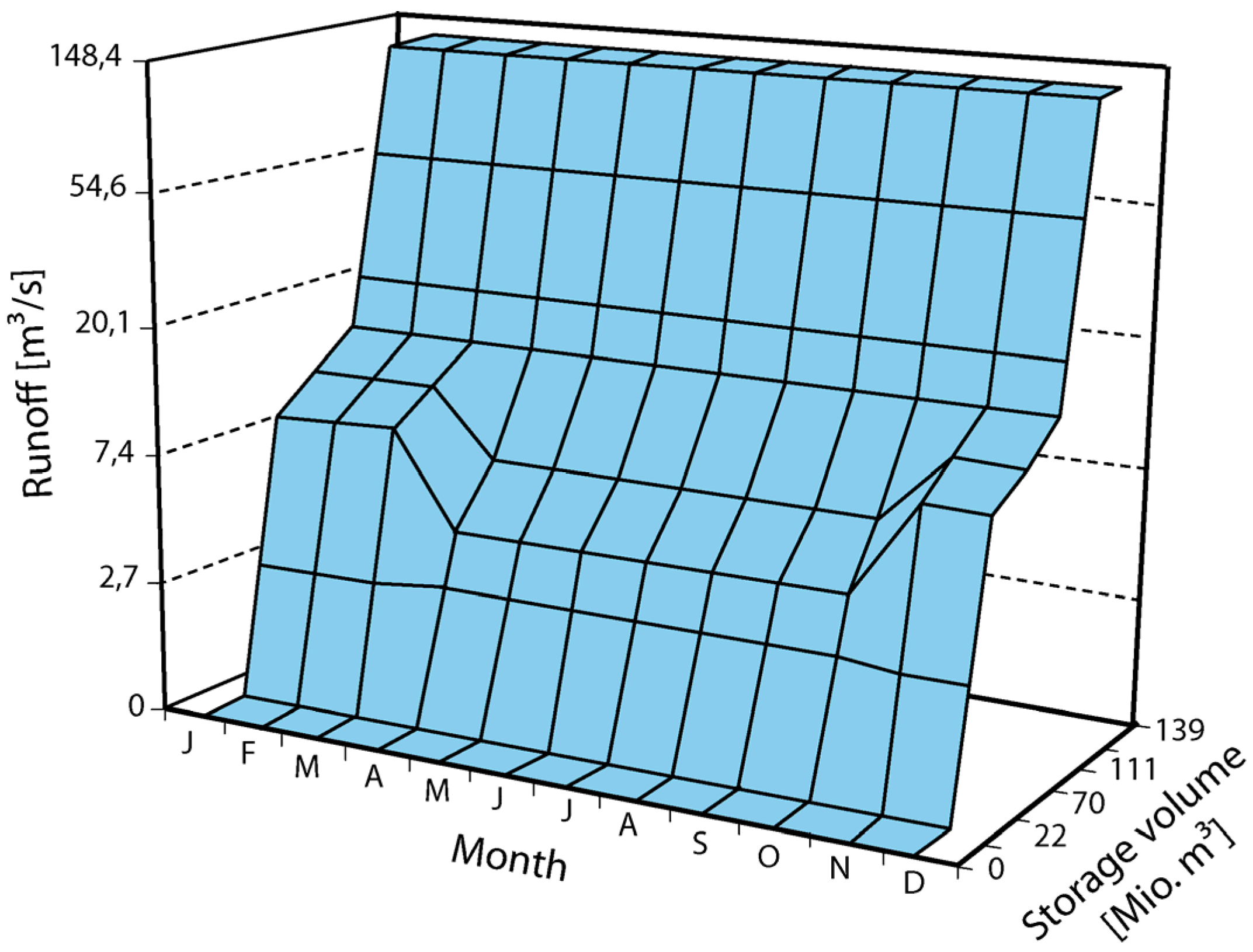
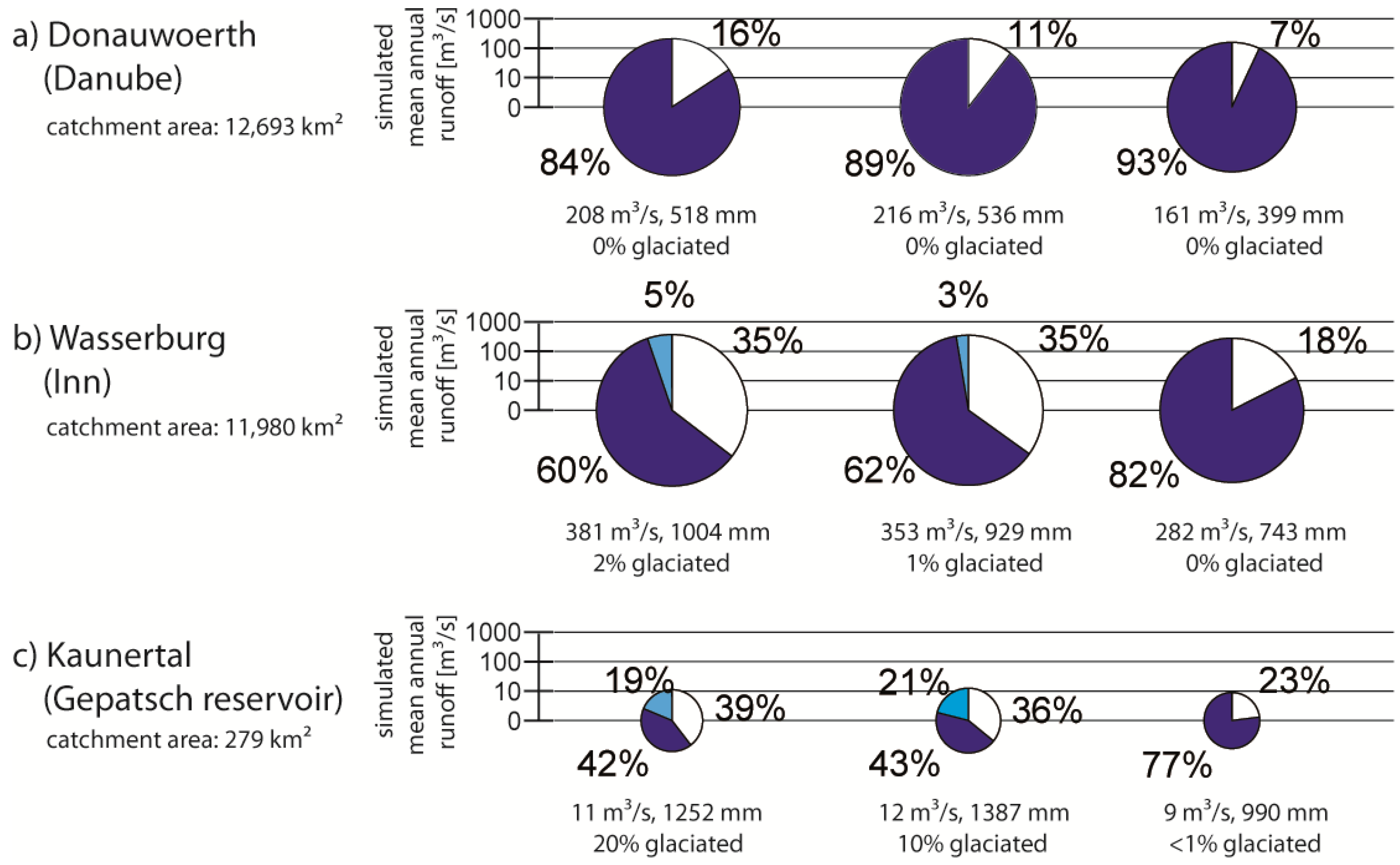
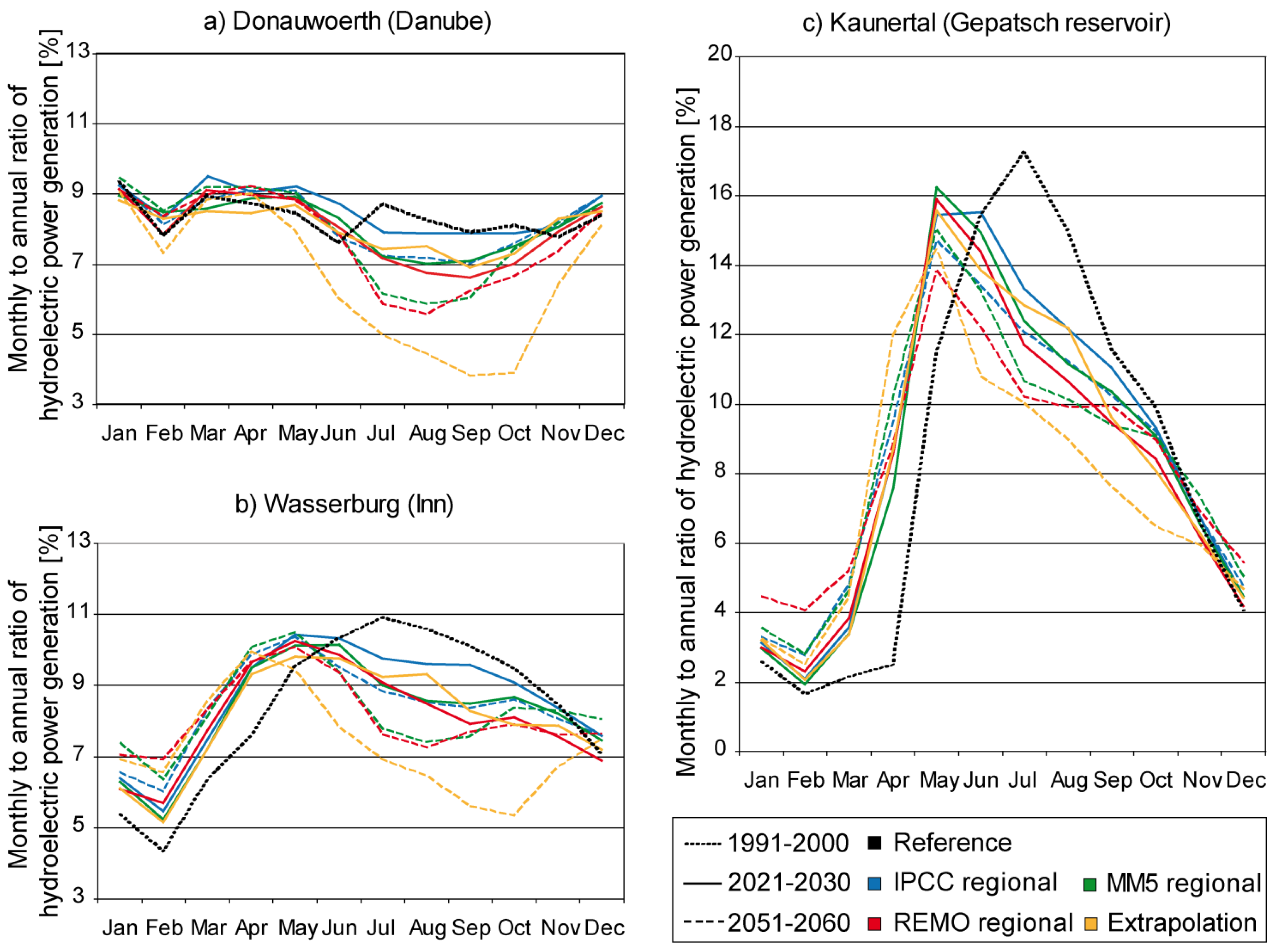
Figure 3 shows the operation scenario for the Gepatsch reservoir. It is the second-largest man-made reservoir in the watershed, located in a glaciated, highly alpine characterized head-watershed and contains a total volume of 139 million m³ of water. The operation scenario considers the runoff components snow- and ice-melt. This means that in times with high melting rates (May to October) more water will be stored by discharging less runoff at the same storage volume than in months with smaller or zero melting rates (November to April). From
Figure 3 it becomes clear that, although principally possible in the module, the operation scenarios do not reproduce the actual operation of these reservoir power plants, which to a certain degree depend on the actual energy demand.
Figure 3.
Monthly-based look-up table plan of the operation of the Gepatsch reservoir.
Figure 3.
Monthly-based look-up table plan of the operation of the Gepatsch reservoir.
3.2. The Hydropower Module
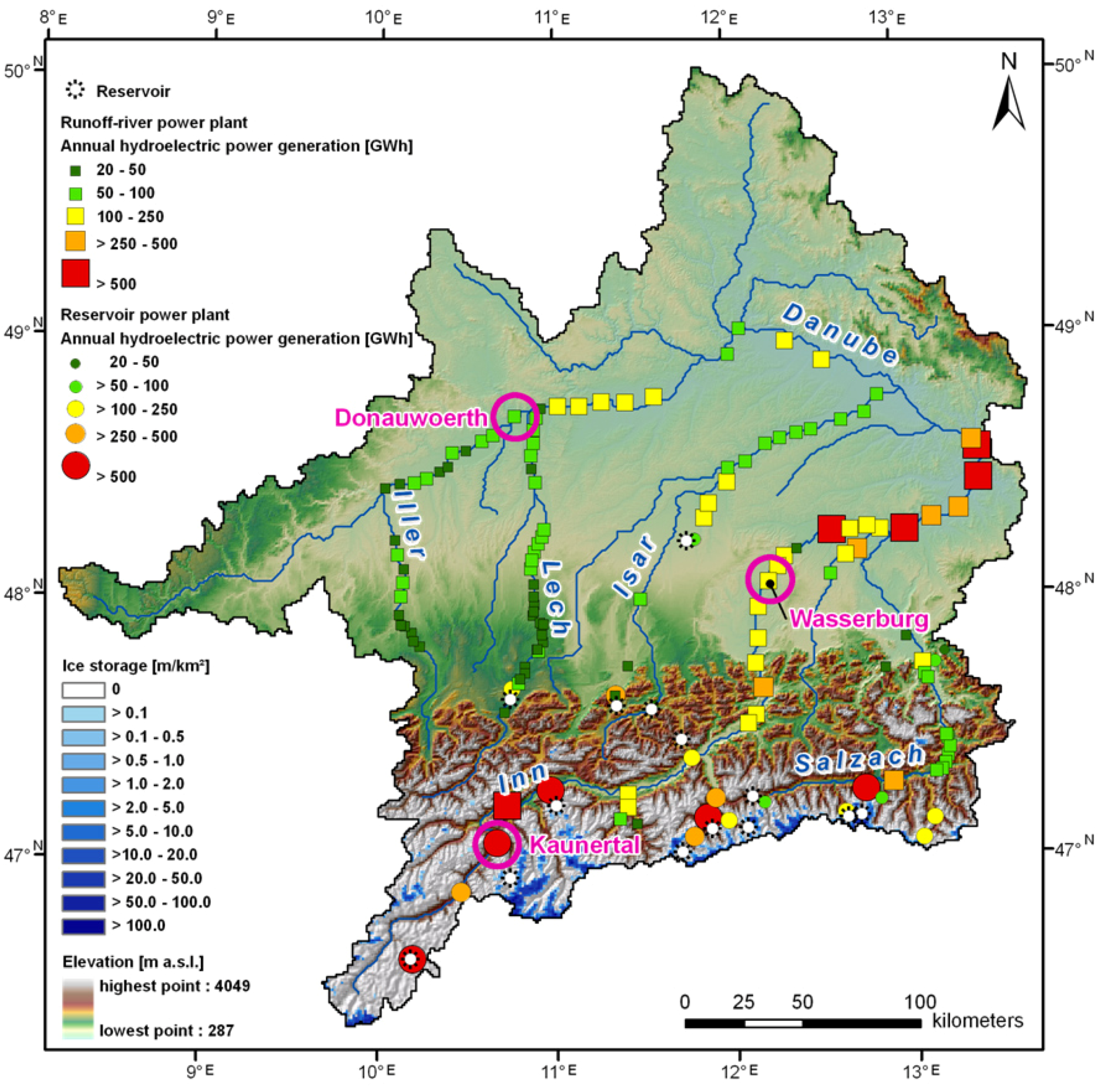
All currently existing hydropower plants with a bottleneck capacity of more than 5 MW (see
Figure 2) are implemented in the hydropower module of PROMET to determine hydroelectric power generation. In general, hydroelectric power generation is based on potential and kinetic energy. Therefore the two most important parameters are runoff and hydraulic head. The capacity of each hydropower plant was calculated with an hourly resolution by the following equation:
where
P is the capacity (for a certain time period) (kW),
η is the efficiency factor of a hydropower plant (-),
ρ is the density of water (kg m
−3),
g is the gravitational acceleration (m s
−2),
Q is the runoff (m
3 s
−1) and
H is the hydraulic head (m). The resulting capacity for each time step was then aggregated to mean daily, annual or decadal hydroelectric power generation values:
where
E is the hydroelectric power generation (kWh),
P is the capacity (for a certain time period) (kW) and
t is the time (h).
Each hydropower plant is located within the investigation area at a defined grid cell of 1 km
2. Hence, for each hydropower plant the runoff
Q referred to the channel flow component is known for each time step. It is the only variable component of Equation (1) changing at each time step. Furthermore, for each of the 118 runoff-river power plants and the 22 reservoir power plants (cf.
Figure 2), the following parameters were investigated and implemented individually: mean annual hydroelectric power generation, hydraulic head, efficiency factor, maximum capacity and starting year of operation of the power station. All data are based on the parameterization derived from the present.
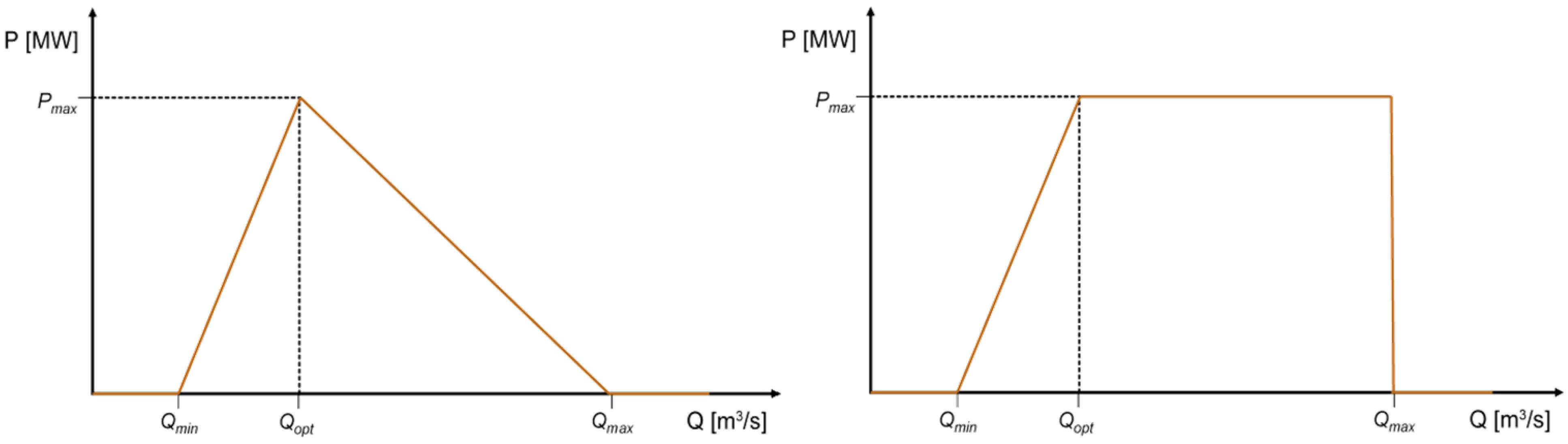
The left side of
Figure 4 illustrates schematically the relationship of capacity
P and runoff
Q for a runoff-river power plant. In general, an increase in channel flow leads to an increase in capacity until the maximum capacity
Pmax at the optimal runoff
Qopt value is reached. For most hydropower plants this point is similar to the maximum discharge of the turbines.
Figure 4.
Relationship of capacity and runoff for runoff-river power plants (left) and for reservoir power plants (right) used in the model.
Figure 4.
Relationship of capacity and runoff for runoff-river power plants (left) and for reservoir power plants (right) used in the model.
The energy generation starts at a minimum channel flow Qmin, which mainly is defined by low-flows and residual flow restrictions. During these situations no energy is produced because low-flows are often not discharged through the turbines. For the runoff-river power plants it is assumed that after achieving Pmax, the capacity decreases because more runoff leads to a rising downstream water level, which results in turn in a reduction of the hydraulic head. After reaching a set maximum channel flow Qmax, the energy production is shut down taking restrictions of energy generation by extreme flood events into account. Overall, this scheme clearly shows that although the capacity is strongly related to the channel flow, low-flow and flood events also have a large impact on capacity.
The relationship of capacity and runoff for a reservoir power plant is handled quite similarly and is shown schematically on the right of
Figure 4. The difference is that after reaching
Qopt,
Pmax is held constant for a longer time, because a rising downstream water level has less influence. Furthermore, each reservoir power plant underlies monthly-based operating rules (see
Section 3.1).
3.3. Validation
As the output of the hydropower module—the capacity or rather the hydroelectric power generation—is highly dependent on channel flow and extreme events like low-flows and floods, the hydrological model PROMET was validated using streamflow records at the outlet gauge Achleiten and several other gauges within the catchment on daily and annual time steps. The respective main validation results will be shortly outlined in the following; a detailed description is handled in Mauser and Bach [
32]. The validation period for the runoff generated by PROMET is a 33-year model run covering the hydrological years (November-October) 1971 to 2003 with an hourly time step. This takes into account the standard climate period 1971–2000 with the extension of the extremely warm Central European Summer of 2003. The hourly runoff was generated for each 1 km
2 pixel and aggregated to daily and annual values for further analysis. Firstly, the annual water balance was compared to the measured annual runoff at the outlet gauge at Achleiten (see
Figure 5) through a linear regression analysis. Since the model should ideally reproduce the measured values the model
y =
a ×
x was taken as regression hypothesis. Both the slope and the coefficient of determination
R2 should be as close as possible to a value of 1 to ensure that the model reproduces the full dynamic of the measured data without any model bias [
37]. The mean modelled runoff at the Achleiten outlet gauge (598 mm/a) compares well with the measured runoff (579 mm/a) [
32]. Secondly, the validation of the short term runoff dynamics the measured versus modelled average daily runoff of the 33-years period was also compared at selected gauges in the watershed, by calculating slopes of linear regression lines forced through the origin, coefficients of determination and Nash-Sutcliffe efficiency coefficients [
48]. The slopes of the regression lines detect systematic biases in the representation of the natural runoff dynamic by the model. The coefficients of determination give an indication of the amount of variance of the measured data, which is captured by the model simulation. The Nash-Sutcliffe efficiency coefficient compares the mean square error generated by a particular model simulation to the variance of the target output sequence. It is defined as:
where
E is the Nash-Sutcliffe efficiency coefficient,
Q0, the measured runoff (m
3/s),
the mean measured runoff (m
3/s), the modelled runoff
Qm (m
3/s),
T the time period and
t the selected time step. An efficiency of 1 corresponds to a perfect match of modelled discharge to the observed data. An efficiency of 0 indicates that the model predictions are as accurate as the mean of the observed data, whereas efficiency less than zero occur when the observed mean is a better predictor than the model. The closer the model efficiency is to 1, the more accurately the model reproduces the data. This normalized measure is used to assess the predictive power of hydrological models; however it does not measure how good a model is in absolute terms. Additionally it should be mentioned that reliability of the Nash-Sutcliffe efficiency coefficient depends on the seasonality of the time series. The model performance for strongly seasonal time series, e.g., glacial regimes, can be overestimated. For time series with small fluctuations around the mean value, this coefficient is a rather good predictor [
49].
Figure 5.
Mean modelled water balance in the Upper Danube watershed during the period 1971 to 2003 and mean measured discharge at the Achleiten outlet gauge (based on Mauser and Bach [
32]).
Figure 5.
Mean modelled water balance in the Upper Danube watershed during the period 1971 to 2003 and mean measured discharge at the Achleiten outlet gauge (based on Mauser and Bach [
32]).
This analysis was executed at a broad range of different gauges of sub-watersheds at different places in the Upper Danube basin and is summarized together with the results from the analysis of the annual runoffs in
Table 1. In general the slopes of the linear regression are close to 1 and the coefficients of determination are high, which indicate that the inter-annual and daily runoff dynamics are well captured by PROMET, both, at the outlet in Achleiten as well as in the sub-watersheds. The coefficient of determination is slightly higher for larger (sub-)watersheds. Accordingly, for the smallest selected watershed the 1 km × 1 km resolution may not be sufficient for this model’s settings and input data. Extreme events, namely low-flows and floods, have influence on the hydroelectric power generation of the hydropower module. The validation of low-flows and floods was carried out at the Achleiten outlet gauge for the same time period. The flood analysis considered the annual peak discharge, whereas the low-flow analysis considered the annual lowest 7-day average flow. Regarding the flood analysis a fairly stable relation was found, nevertheless an overestimation by 16% of the simulated values was shown because of neglecting inundations and dam breaks during very large floods. However, the simulated and measured low-flow frequency correlated very well. This also applies to the return periods of both extreme events [
32]. In general, PROMET, which is not adjusted to observed runoff, is able to model the flow within the channel network and the extreme events low-flows and floods, by agreeing well up, to very well with measured values. Since the runoff is the only variable input of Equation (1) (see
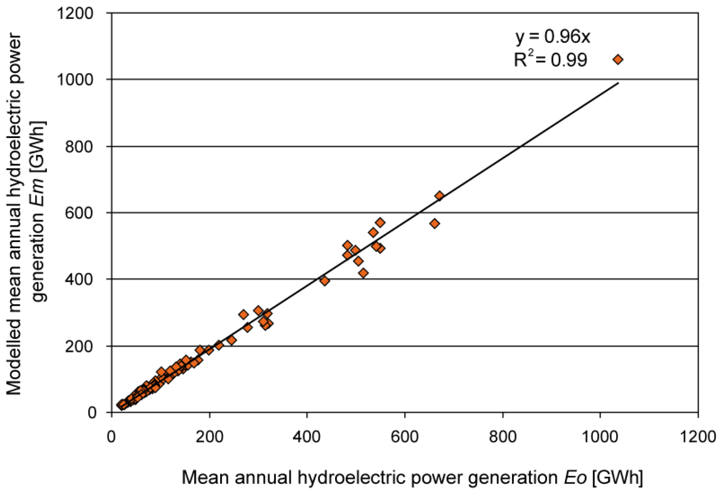
Section 3.2), the hydroelectric power generation is well displayed. The mean annual hydroelectric power generation
Em calculated with PROMET has been validated for each power plant with the mean annual hydroelectric power generation
Eo published by the hydropower plant operators.
Table 1.
Statistical analysis by calculating slopes of linear regression lines, coefficients of determination and the Nash-Sutcliffe coefficient (only for the daily values) for the linear correlation between the modelled and measured annual and daily runoff of selected (sub-)watersheds in the Upper Danube basin in the period 1971–2003 (based on Mauser and Bach [
32]).
Table 1.
Statistical analysis by calculating slopes of linear regression lines, coefficients of determination and the Nash-Sutcliffe coefficient (only for the daily values) for the linear correlation between the modelled and measured annual and daily runoff of selected (sub-)watersheds in the Upper Danube basin in the period 1971–2003 (based on Mauser and Bach [32]).
| | Annual Values | Daily Values |
|---|
| Gauge name | River | Size of (sub-) watershed | Slope of linear regression | Coefficient of determination | Slope of linear regression | Coefficient of determination | Nash-Sutcliffe efficiency coefficient |
|---|
| Achleiten | Danube | 76,660 km2 | 1.05 | 0.93 | 1.03 | 0.87 | 0.84 |
| Hofkirchen | Danube | 46,496 km2 | 1.12 | 0.93 | 1.11 | 0.87 | 0.81 |
| Dillingen | Danube | 11,350 km2 | 1.14 | 0.93 | 1.13 | 0.84 | 0.72 |
| Oberaudorf | Inn | 9715 km2 | 0.99 | 0.80 | 0.94 | 0.81 | 0.80 |
| Plattling | Isar | 8435 km2 | 1.03 | 0.88 | 1.08 | 0.75 | 0.47 |
| Laufen | Salzach | 6112 km2 | 0.93 | 0.85 | 0.86 | 0.85 | 0.80 |
| Heitzenhofen | Naab | 5431 km2 | 1.01 | 0.86 | 0.99 | 0.78 | 0.79 |
| Weilheim | Ammer | 607 km2 | 1.09 | 0.88 | 0.98 | 0.63 | 0.69 |
This data was further confirmed by literature, websites and technical papers. The conducted validation of the mean annual values shows a very good correlation with a high coefficient of determination
R2 (0.99) on a long term basis (
Figure 6).
Figure 6.
Validation of the mean annual hydroelectric power generation by comparing the model output data (Em) with information from the hydropower plant operators (Eo) for all considered hydropower plants in the Upper Danube basin for the time period 2000–2006.
Figure 6.
Validation of the mean annual hydroelectric power generation by comparing the model output data (Em) with information from the hydropower plant operators (Eo) for all considered hydropower plants in the Upper Danube basin for the time period 2000–2006.
The time period 2000 to 2006 was chosen, because since 2000 nearly all hydropower plants integrated in the model had started with the energy production and the meteorological driver data for the model was available until 2006 (see
Section 3.4). Regarding the relationship
Em/
Eo the mean (0.96) is close to the value 1. The root mean square error (0.08) and the variance (0.01) have low values. This statistical analysis shows that the hydropower plants in the hydropower module are well reproduced for the mean annual values by the simulation.
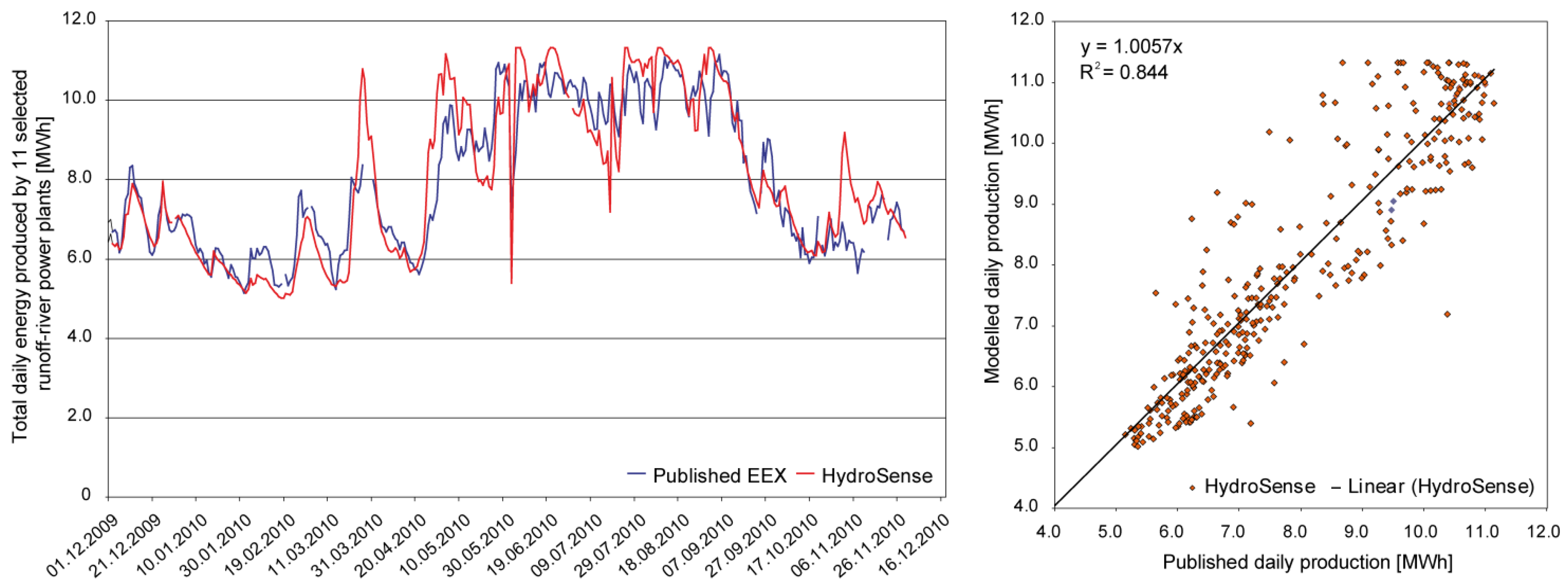
To further prove the hydroelectric power generation calculated with PROMET, daily production rates as published by the EEX energy stock exchange were consulted and used for validation of the model results. Validation on a finer temporal resolution was performed within the “HydroSense” service by VISTA Remote Sensing in Geosciences GmbH, providing analyses and forecasts of hydropower generation based on PROMET calculation on an operational basis [
50]. Based on a dense net of meteorological stations, provided by the private weather data service EWC, hourly and daily results of modeled runoff and hydropower production were created. As validation datasets, hourly published energy production of the EEX energy stock exchange [
51] for the year 2010 was taken into consideration. These published datasets are based on a voluntary commitment of the main energy providers in Germany and Austria. Due to publishing structure, only the sum of energy production of 11 river-runoff power plants is provided by the EEX database. A comparison of the cumulated daily energy production for these 11 runoff-river power plants modelled with PROMET at the rivers Danube and Inn for the year 2010 is presented in
Figure 7. Modelled daily production (red line) follows the published values (blue line) during the entire year and shows a very good correlation (
y = 1.0057
x;
R2 = 0.84).
A further analysis, comprising single power plants or reasonable hourly resolution, will be possible when more detailed information on energy production for river-runoff and reservoir hydropower, will be provided by the energy providers.
Figure 7.
Total daily sum of 11 analysed runoff-river power plants located at the rivers Danube and Inn. Comparison of modelled HydroSense and published EEX hydroelectric power generation data.
Figure 7.
Total daily sum of 11 analysed runoff-river power plants located at the rivers Danube and Inn. Comparison of modelled HydroSense and published EEX hydroelectric power generation data.
3.4. Meteorological Input Data and Climate Trends
The hydrological model PROMET requires meteorological driver data for each grid cell and each time step. To conduct past and future simulations, data for a past period (1960–2006) and for a future period (2011–2060) were set up during the GLOWA-Danube project. The generation and the specifications of the meteorological input data will be described in the following sections.
The past meteorological data set is derived from 277 climatologic stations from the standard network of the German (DWD) and Austrian (ZAMG) Weather Services. The investigated meteorological variables for each grid cell on a 1 km
2 scale and an hourly time step are precipitation, air temperature, humidity, radiation, horizontal wind speed and air pressure. Therefore, firstly a cubic spline interpolation was used to generate hourly values out of the three standard daily records (7 a.m., 2 p.m. and 9 p.m.) of each meteorological station. Secondly, the spatial interpolation was carried out taking altitudinal gradients and a digital terrain model into account (see [
32,
36]).
The meteorological data set for the future was generated by using a stochastic climate generator [
32,
52], recombining the historical dataset, considering statistically different predefined climate trends. This generator is classified as a stochastic nearest neighbour climate generator similar to the approaches of Orlowsky
et al. [
53], Yates
et al. [
54], Buishand and Brandsma [
55] and Young [
56]. It produces a likely realisation of future climate and not synthetic weather data for regions with sparse data available like WGEN [
57] or LARS-WG [
58,
59]. It is assumed that the annual course of a year can be decomposed into weeks represented by temperature means, precipitation sums and their covariance. This climate generator produces weekly sequences of temperature means, precipitation sums and their covariance out of historic data and reassembles them randomly by an underlying climate trend on temperature and precipitation for the future time period. The outputs are new, synthetic time series with the same temporal and spatial resolution as the input data, whereby the physical relations between the meteorological variables are restored. At present stage, future precipitation can be better represented with the climate generator than with most direct regional climate model (RCM) simulations. Another advantage of the climate generator is that the future scenario climate data need no bias correction because it uses the change signal and not RCM data series directly. It should be kept in mind, however, that the general statistical relationship of temperature and precipitation is assumed not to change in future [
32]. Regarding the limits of the climate change generator, e.g., a future change in weather patterns, however, can not be considered appropriately with this tool.
To identify possible future changes and to cover a plausible range of uncertainties in regional climate development, 16 climate scenarios, resulting from different ensemble outputs of the stochastic climate generator, were taken as meteorological drivers for the period 2011–2060. All climate scenarios are based on the global IPCC-SRES-A1B emission scenario, which shows a mean development of greenhouse gas emissions due to mid-line economic growth [
1], and are part of four regional climate trends. For each of the four trends, four climate scenarios have been selected on statistical criteria. They follow different approaches and are named thereafter
IPCC regional,
REMO regional MM5 regional, and
Extrapolation. The
IPCC regional climate trend is based on the results from 21 global climate models for Central Europe presented in the latest IPCC report [
1]. The REMO regional trend underlies the application of the RCM REMO driven by ECHAM5 [
60], which is applied in several studies in this region [
8,
21,
60,
61,
62]. Among other RCMs, REMO represents a moderate temperature and precipitation development [
63,
64]. Several RCMs underestimate for example the summer drying especially in the Danube region. REMO, however, shows a very modest bias [
64]. To cover a range of uncertainties a second RCM trend, the
MM5 regional trend, which is based on the application of the regional climate model MM5 and is also driven by ECHAM5 [
65], was applied. The background of the
Extrapolation trend is the analysis of temperature and precipitation trends of historic climate stations data of the German (DWD) and Austrian (ZAMG) weather services, analysed by Reiter
et al. [
66].
To show the characteristic development of the meteorological input data,
Table 2 gives an overview of the temperature and precipitation changes between 1990 and 2100 regarding the four climate trends considering annual and semi-annual summer (May–October) and winter (November–April) periods. For the annual values all trends show a clear increase in temperature and a varying decline in precipitation until 2100. In general, the
IPCC regional trend is the weakest, followed by the rather moderate trends
MM5 regional and
REMO regional. The
Extrapolation trend is the most severe one. For all four trends temperature increase results in less annual precipitation with a clear decrease in summer and a slighter increase in winter. Thereby, comparing the middle trends,
REMO regional shows a slightly higher decrease in summer and a smaller increase in winter than
MM5 regional.
Table 2.
Temperature increase (K) and precipitation changes (%) between 1990 and 2100 regarding the four climate trends IPCC regional, MM5 regional, REMO regional and Extrapolation.
Table 2.
Temperature increase (K) and precipitation changes (%) between 1990 and 2100 regarding the four climate trends IPCC regional, MM5 regional, REMO regional and Extrapolation.
| Climate Trend | Temperature Increase (K) | Precipitation Changes (%) |
|---|
| Annual | Annual | Winter (November–April) | Summer (May–October) |
|---|
| IPCC regional | +3.3 | −4.4 | +2.1 | −10.2 |
| MM5 regional | +4.7 | −3.5 | +10.1 | −14.6 |
| REMO regional | +5.2 | −12.6 | +7.3 | −16.6 |
| Extrapolation | +5.2 | −16.4 | +9.0 | −30.7 |
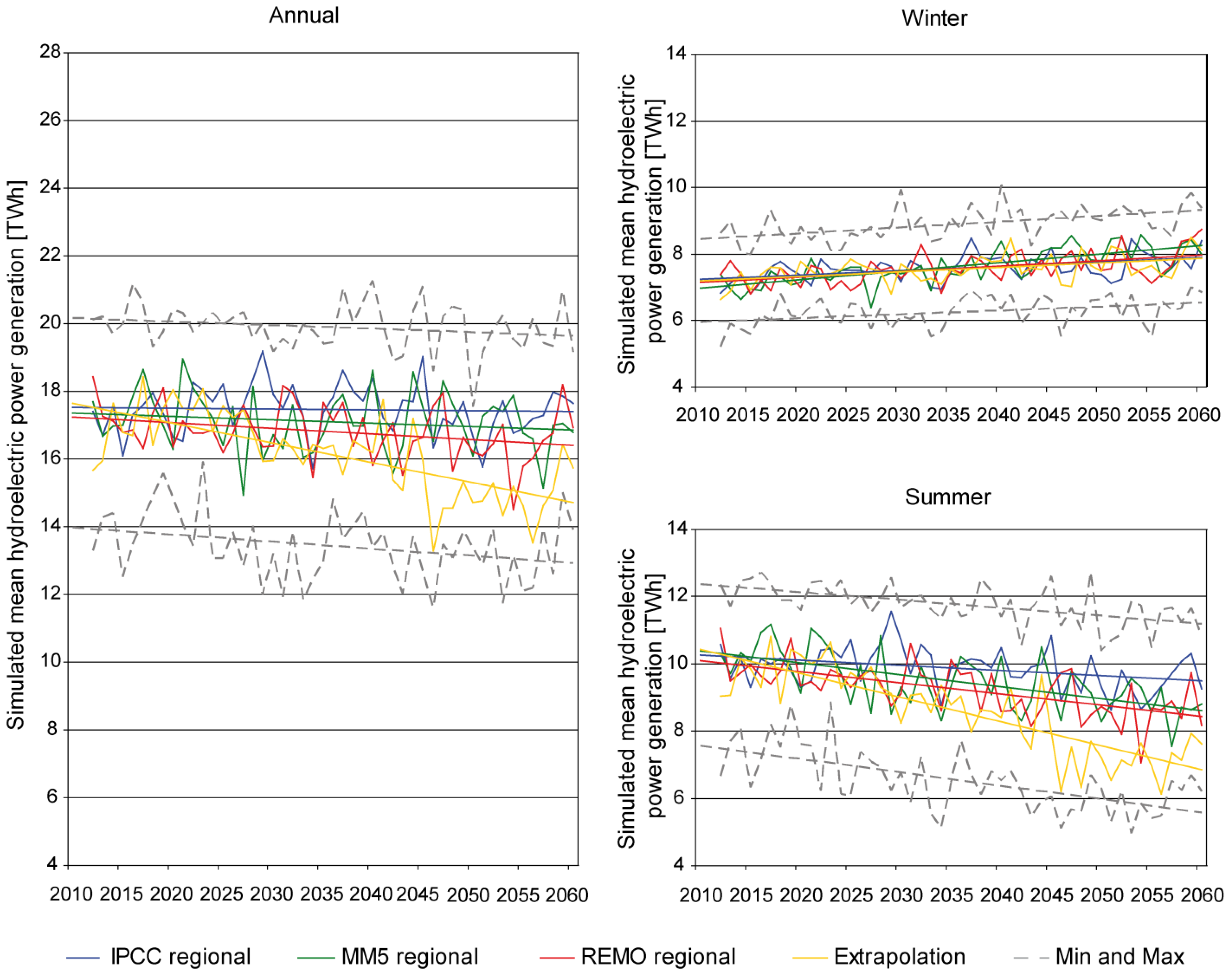
As shown in
Section 4.1, the temperature and precipitation changes of each trend trigger in turn by a more or less extent, changes in runoff, the hydrological storage and thereafter also in hydroelectric power generation.

 and
and 


