Global Assessment of High-Altitude Wind Power

Abstract

The available wind power resource worldwide at altitudes between 500 and 12,000 m above ground is assessed for the first time. Twenty-eight years of wind data from the reanalyses by the National Centers for Environmental Prediction and the Department of Energy are analyzed and interpolated to study geographical distributions and persistency of winds at all altitudes. Furthermore, intermittency issues and global climate effects of large-scale extraction of energy from high-altitude winds are investigated.

1. Introduction

Winds generally increase with height above the ground [1]. The jet streams, meandering currents of fast winds generally located between 7 and 16 km of altitude [2], have wind speeds that are an order of magnitude faster than those near the ground. Two jet streams exist in each hemisphere: the “polar jet stream”, found over the mid-latitudes at altitudes of 7-12 km, and the weaker “sub-tropical jet stream”, found near ± 30º at greater altitudes (10-16 km).

Despite seasonal shifts, the jet streams are relatively persistent features of the mid-latitudes in both hemispheres. The total wind energy in the jet streams is roughly 100 times the global energy demand [3]. Because of their abundance, strength, and relative persistency, jet stream winds are of particular interest in wind power development.

Several technologies have been proposed that aim at harnessing wind power at high altitudes. Most of them are still at an early stage of development, in which patents have been obtained but neither a business entity nor a commercial-scale prototype exist. No high-altitude wind power technology to date has produced a prototype that has been tested long enough to provide a solid record of electricity generation and associated costs.

Two basic approaches have been proposed. Mechanical energy can be transmitted from altitude to the Earth’s surface, where generators would produce electricity at the ground. An example is the design of KiteGen (Figure 1a), consisting of tethered airfoils (kites) connected to a ground-based generator with two lines, which are pulled and released by a control unit [4,5,6]. The energy generated during the traction phase is greater than the energy needed in the recovery phase. A single unit of 100 m² is expected to generate 620 kW of electricity; arrays of several kites can be arranged in a carousel configuration around a circular rail for electricity generation of up to 100 MW. This approach appears most suitable for the lowest few km of the atmosphere.

Alternatively, electricity could be generated aloft and transmitted to the surface with a tether. In the design proposed by Sky Windpower (Figure 1b), four rotors are mounted on an airframe, tethered to the ground via insulated aluminum conductors wound with Kevlar-type cords [3]. The rotors both provide lift and power electric generation. The aircraft can be lofted with supplied electricity to reach the desired altitude, but then can generate up to 40 MW of power, with angles of up to 50° into the wind. Multiple high altitude wind turbines (rotorcrafts) could be arranged in arrays for large scale electricity generation. For this approach, the aim would be to capture energy closer to the jet streams.

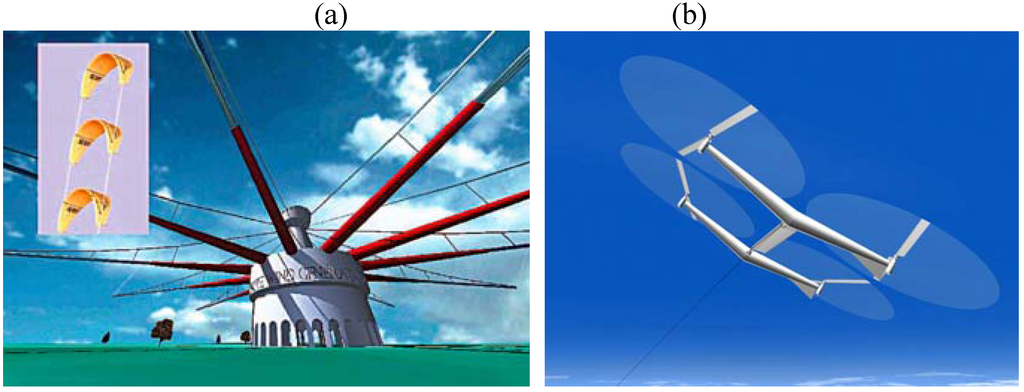
Figure 1. Examples of high-altitude technologies: (a) KiteGen, kites aimed at altitudes of 1000 m and tethered to a spinning carousel at the ground; and (b) Flying Electric Generators by Sky Windpower, tethered rotorcrafts aimed at altitudes of 10,000 m (picture courtesy of Ben Shepard).

Figure 1. Examples of high-altitude technologies: (a) KiteGen, kites aimed at altitudes of 1000 m and tethered to a spinning carousel at the ground; and (b) Flying Electric Generators by Sky Windpower, tethered rotorcrafts aimed at altitudes of 10,000 m (picture courtesy of Ben Shepard).

2. Methods and Data

The amount of power that can be captured by a wind turbine is a function of wind speed (V) and density (ρ) of the air going through the blades [7]. Wind speed generally increases with height above the boundary layer, while air density decreases nearly exponentially [1]. Wind power density (δ) takes these two competing effects into account and represents the wind power available per unit of area swept by the blades (W/m²):

(1)

To calculate wind power density throughout the troposphere, we used reanalyses of wind speed, temperature, pressure, and specific humidity from the National Centers for Environmental Prediction (NCEP) and the Department of Energy (DOE), with a temporal frequency of 6-hours, from 1979 to 2006 [8]. These reanalyses have 192 x 94 grid points in the horizontal, with spacing of ~1.9 degrees. Whereas this resolution is adequate for resolving upper level winds [2,9], it is relatively coarse to fully capture the features of winds in the lower 1-2 km. Because the NCEP/DOE reanalyses incorporate all available wind measurements from radiosondes worldwide, they are the most reliable source of gridded upper level winds available, although positive biases have been reported in the observation-sparse Arctic region [10]. The meteorological fields were originally on 28 sigma levels. The vertical coordinate sigma is defined as the ratio of the current level’s pressure over the surface pressure. Assuming a standard atmosphere and no moisture, the 28 original sigma levels were approximately at (in m above ground): 42, 152, 304, 496, 734, 1,029, 1,389, 1,827, 2,351, 2,970, 3,692, 4,518, 5,447, 6,476, 7,596, 8,793, 10,059, 11,376, 12,740, 14,136, 15,562, 17,019, 18,527, 20,084, 21,741, 23,606, 25,818, and 29,921, and were linearly interpolated to the following levels (in m above ground): 500, 750, 1,000, 1,500, 2,000, 3,000, 4,000, 5,000, 6,000, 7,000, 8,000, 9,000, 10,000, 11,000, and 12,000. Values at 80 m were calculated with the Least Square Error methodology [11,12] to better represent boundary-layer effects. Here we focus on the 1,000 and 10,000 m levels, representative of targets for ground-based and aloft-based electricity generation approaches, respectively.

Although the power in winds is not a function of wind direction, a variety of safety issues, such as interference with aviation operations, are associated with changes in wind direction. Furthermore, wind direction affects the operation and control of high-altitude devices [13]. A common practice is to obtain clearance over a circular area of radius equal to the tether length, regardless of the wind direction. Because wind direction affects safety and control issues of high-altitude wind devices, but not wind energy availability, in this paper we focus on wind speed and wind power density.

3. Geographical and Statistical Distributions

The amount of energy in high altitude winds, and its intermittency, depend on the frequency distribution of wind power density. Because wind power density is proportional to the third power of wind speed (Equation 1), fluctuations of wind speed greatly affect wind power output. Furthermore, turbines often cannot capture energy in either the strongest or the weakest winds. Hence, we do not focus on mean values, but rather on a few percentiles (50^th or median, 68^th, and 95^th), which indicate the wind power density that is exceeded on 50%, 68%, and 95% of the time during 1979-2006.

3.1. Global Vertical Profiles

First, we analyze the profile of global average wind power density by level (Figure 2a), obtained by averaging, for each percentile, the wind power density over all latitudes and longitudes. The highest wind power densities are found at altitudes between 8,000 and 10,000 m above ground, corresponding roughly to the height of the tropopause. The 10,000 m altitude appears to be the maximum height that is worth exploring for high-altitude wind power technologies.

Whereas above 2,000 m wind power density increases monotonically with height, the altitude range between 500 and 2,000 m has relatively constant wind power densities, with actually a slight decline between 500 and 1,500 m for median and slower winds (i.e., winds available ≥ 50% of the time). This finding, consistent with [5, 6] for several sites in Europe, suggests that, on average, there may not be much benefit in going higher than 500 m, unless reaching above 2,000 m.

Although the most rapid increase in wind power density with altitude occurs between 6,000 and 7,000 m (for median winds, +0.37 W/m² for each m increase in altitude), going from 80 to 500 m also gives a significant increase in wind power density (+0.25 W/m²/m for median winds).

Figure 2. Wind power density (kW/m²) that was exceeded 5%, 32%, 50%, 68%, and 95% of the time during 1979-2006 as a function of altitude from the NCEP/DOE reanalyses [8]. The profiles at the five largest cities in the world are shown in (b-f). The global average profile (a) is the area weighted mean of values like those represented in panels (b) through (f) at all grid points.

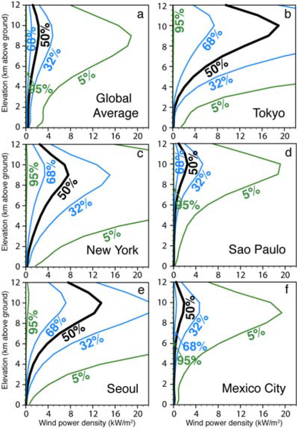
Figure 2. Wind power density (kW/m²) that was exceeded 5%, 32%, 50%, 68%, and 95% of the time during 1979-2006 as a function of altitude from the NCEP/DOE reanalyses [8]. The profiles at the five largest cities in the world are shown in (b-f). The global average profile (a) is the area weighted mean of values like those represented in panels (b) through (f) at all grid points.

While more consistent than low-altitude winds, high-altitude winds are not steady and strong all the time. For example, 5% of the time wind power density is low (<0.1 kW/m²) in most places, less than 1/10 of the median density. Also, the wind power density distribution is non-symmetric, with a long tail towards higher power densities. This can be inferred, for example, from the larger difference between the values of the 5% and the 50% percentiles versus the smaller difference between the 50% and the 95% percentiles in Figure 2 at all locations and all levels, but especially near the jets.

3.2. City Vertical Profiles

For comparison, we show in Figures 2(b-f) the profiles of wind power density at the five largest cities in the world, i.e., Tokyo (33.2 million people), New York (17.8), Sao Paulo (17.7), Seoul (17.5), and Mexico City (17.4). For cities that are affected by polar jet streams (e.g., Tokyo, Seoul, and New York), the high-altitude resource is phenomenal, with wind power densities greater than 10 kW/m² for more than 50% of the time at ~8,000 m. New York is the city with the highest average wind power density near the jet (11.6 to 16.3 kW/m²) in the U.S., based on observed sounding profiles [14]. Tokyo and Seoul present similar vertical profiles of wind power density because they are both affected by the East Asian jet stream [15,16]. Because Mexico City and Sao Paulo are located at tropical latitudes, they are rarely affected by the polar jet streams and occasionally by the weaker sub-tropical jets, and thus have lower wind power densities than the other three cities.

3.3. Atlas

To account for local and seasonal variations in the wind resource, we prepared an atlas of selected percentiles of wind power densities for all vertical levels, available in the Supplementary Material Deposit (Figures S1.1-S1.80), a few of which are analyzed here (1,000 and 10,000 m in Figure 3).

Since winds at 1,000 m (Figure 3, left panel) are still affected by surface friction and topography over land, but not over the ocean [17,18], wind power density maxima at 1,000 m are found generally over the oceans, e.g., Southern Ocean, northern Atlantic, northern Pacific, and the Caribbean. Over land, the best location is the tip of South America (median power densities > 1 kW/m²), followed by the horn of Africa and western South America (medians > 0.5 kW/m²). At least 5% of the time, the wind power density resource at 1,000 m is effectively zero over land.

Wind power density at 10,000 m (Figure 3, right panel) is on average over five times larger than that at 1,000 m (i.e., the global area-average of the median wind power densities at 1,000 and 10,000 m are 422 and 2,282 W/m² respectively). At 10,000 m, the locations with the highest wind power densities are strongly correlated with the locations most frequently visited by the jet streams [2]: to the east of North America and Asia, the Southern Ocean between Africa and Antarctica, north Africa, and to the east of Australia. Even over Japan, possibly the best location worldwide for high-altitude wind power, the wind power density falls below 0.5 kW/m² 5% of the time – a relatively small fraction of the median power density (>10 kW/m²). This suggests again that the intermittency problem that affects wind power near the ground might not be completely solved by high-altitude wind power.

Seasonal differences were found at all levels. In the boreal summer, a clockwise band of high wind power density at 1,000 m, associated with the monsoon, can be seen over the Indian Ocean (Figure S1.52), with maxima to the south-east of the Arabian Peninsula, consistent with the onset of the Somali low-level jet [19]. At 10,000 m, a broad area of high wind power density over the Indian Ocean in the boreal summer (Figure S1.52) reflects the presence of the easterly jet associated with the monsoon [19].

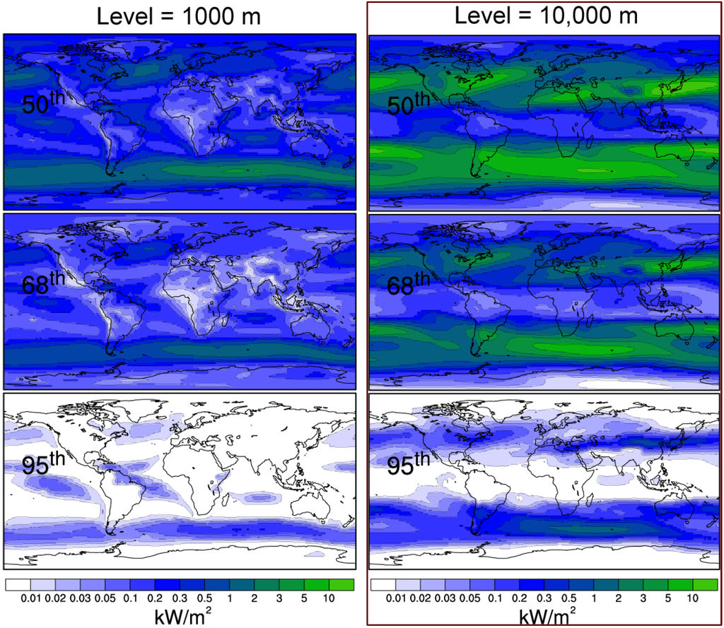
Figure 3. Wind power density (kW/m²) that was exceeded 50%, 68%, and 95% of the time during 1979-2006 at 1,000 m (left) and 10,000 m (right) from the NCEP/DOE reanalyses [8].

Figure 3. Wind power density (kW/m²) that was exceeded 50%, 68%, and 95% of the time during 1979-2006 at 1,000 m (left) and 10,000 m (right) from the NCEP/DOE reanalyses [8].

In each hemisphere’s winter, wind power density patterns are generally similar to the annual patterns, but the bands of high winds at the mid-latitudes near 10,000 m are generally broader, extend further equatorward, and have higher wind speeds (Figure S1.30).

3.4. Optimal Height

Although in general wind speed increases with height, altitudes at which winds are strongest can vary, depending on the weather conditions. For example, low-level jets cause wind maxima at the top of the boundary layer [20], ~1,000 m above ground. Obvious benefits would arise if a high-altitude technology were able to dynamically reach this “optimal” height. First, harnessing the maximum wind power possible at a given location by reaching the optimal height increases the capacity factor, which is the ratio of actual generated over rated power, when compared to the capacity ratio at a fixed altitude. Also, the intermittency problem (i.e., periods with low wind power densities) at a specific location and altitude can be ameliorated by lifting or lowering the kites to avoid low wind speeds.

From the NCEP/DOE reanalyses, we calculated optimal height and optimal wind power density for each grid point and corresponding statistics for the 1979-2006 period. Overall, 95% of the time the optimal wind power density (Figure 4e) is >0.2 kW/m² over most of the populated land and the optimal height is <6,000 m. This means that, at an average inland location, 95% of the time the high-altitude wind power density available is greater than the median wind power density at windy offshore locations near ground (Figure S1.1).

Areas with the highest median optimal power density are also, in general, the ones with most reliable winds, because of the high power expected to be available 95% of the time. For example, the area of optimal wind power density > 10 kW/m² to the east of Asia near Japan (Figure 4a) experiences wind power densities of at least 1 kW/m² 95% of the time (Figure 4e), practically unthinkable near the ground even at the windiest spots. The optimal altitudes, however, are generally high, above 6 km 95% of the time (Figure 4f).

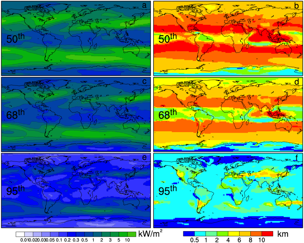
Figure 4. Optimal wind power density (kW/m², left panels) and optimal height (km, right panels) that was exceeded 50%, 68%, and 95% of the times during years in 1979-2006 from the NCEP/DOE reanalyses

Figure 4. Optimal wind power density (kW/m², left panels) and optimal height (km, right panels) that was exceeded 50%, 68%, and 95% of the times during years in 1979-2006 from the NCEP/DOE reanalyses

At lower altitudes, other areas can be of interest. For example, the central United States and northern Africa benefit from relatively high power densities (>0.5 kW/m², Figure 4e), with optimal heights that are relatively low (above 500 m, Figure 4f) most of the time (95%).

If the optimal heights can be reached effectively, then the intermittency problem can be greatly reduced, but not eliminated. Going back to the Japan example, the 95^th percentile of optimal wind power density is ~1 kW/m². Although this is a two-fold improvement over the value at 10,000 m discussed earlier (0.5 kW/m²), a fluctuation of one order of magnitude in wind power production is still large for baseload electricity generation.

4. Dealing with Intermittency

To reduce this intermittency problem, i.e., to “firm” the power output, we analyzed three possible approaches: storing energy (in a variety of forms, including batteries, pumped hydroelectric, and compressed air storage) when production exceeds demand and then releasing it when demand exceeds production; increasing the area intercepted by the device (by adding more turbines or kites); and interconnecting devices that are geographically dispersed via ground-based transmission lines [21]. The interplay among these factors is illustrated for an idealized case for New York (Figure 5) at 68%, 95%, and 99.9% reliability (other cities in Figures S3.1-S3.10).

Figure 5. Contours of wind power output per swept area (kW/m²) that can be supplied from optimal high-altitude winds in New York with: (a) 68%, (b) 95%, (c) and 99.9% reliability as a function of battery size (kWh/m², logarithmic scale) and transmission distance (km).

Figure 5. Contours of wind power output per swept area (kW/m²) that can be supplied from optimal high-altitude winds in New York with: (a) 68%, (b) 95%, (c) and 99.9% reliability as a function of battery size (kWh/m², logarithmic scale) and transmission distance (km).

For each reliability level, contours show firm wind power output per unit turbine area generating electricity at the Betz limit [22] as a function of both battery size (per unit area of high-altitude device) and radius of circular area covered with interconnected high-altitude devices. The battery is assumed to have no losses; it charges when production exceeds the desired output and then releases it when it has energy stored and production does not meet the desired output. The effect of interconnection via perfect transmission lines is calculated by averaging the wind power output over increasingly larger circular areas around each city, for radii between 0 and 3,000 km with 200 km increments.

With no storage or transmission in New York, an astonishing 2 kW/m² are provided most (68%) of the time (Figure 5a), but less than 0.1 kW/m² are provided 99.9% of the time (Figure 5c). Adding battery storage always increases supply of reliable power. For small battery sizes (< 100 kWh/m²), we found improvements in both reliability and amount of wind power generated as the transmission distance increases. For larger battery sizes (> 1,000 kWh/m²), the interconnection of far-away sites is still beneficial at non-windy sites (e.g., Figure S3.10), whereas at windy sites, such as New York in Figure 5, it just causes a reduction of wind power output, as less windy sites added to the network tend to discharge the batteries.

Although high-altitude wind power at a given location might not be suitable for baseload power, a smart combination of storage, larger devices, and interconnected systems at appropriate locations might provide firm power. A more detailed evaluation would consider cost optimization and integration with other sources of power.

5. Climate Effects

A final issue is whether large-scale implementation of high-altitude wind power devices, especially near the jet stream level, can alter the general circulation patterns and have significant effects on global and local climate. To bound the problem, a worst-case scenario was designed in which high-altitude devices were laid out uniformly throughout the atmosphere at densities varying between 1 and 10,000 m² of turbine area per km³ of atmosphere. The lower limit of the range (1 m²/km³) represents roughly the device density needed to supply the world’s electricity demand. Each device is assumed to be perfectly efficient and thus extract available kinetic energy of the winds at the Betz limit [22] to then generate electricity that is transmitted to the ground without losses and converted to heat near the surface.

A global climate model considering the atmosphere and the upper ocean [23] was modified to include these effects and run at 2 by 2.5 degree (latitude by longitude) resolution for 70 years, with the last 30 years retained for analysis. Results (Table 1) show negligible climatic effects at low densities (1 m²/km³), but lower surface temperatures (by up to -9 ^oC), decreased precipitation (by 6.5-35.4%), and greater sea ice cover (by 17.1-195.2%) for increasing densities.

Figure 6 shows the increasing sea ice cover near the North Pole as the density of high-altitude devices increases, possibly due to the strengthening of the Equator-to-Pole thermal difference caused by the weakening of the global winds induced by the devices. Further studies are recommended to further explore this interpretation.

Table 1. Differences between the values of global-average parameters from climate runs with high-altitude devices for increasing device areas throughout the entire atmosphere and those from the control case with no such devices. A uniform device density of 1 m²/km³ corresponds roughly to the world’s electricity demand.

	Difference from control case
Device area (m2/km3)	Mean surface temperature (oC)	Sea ice cover (%)	Total precipitation (%)
1	-0.04	+0.45	-0.12
100	-2.17	+17.09	-6.53
10,000	-9.56	+195.19	-35.37

Table 1. Differences between the values of global-average parameters from climate runs with high-altitude devices for increasing device areas throughout the entire atmosphere and those from the control case with no such devices. A uniform device density of 1 m²/km³ corresponds roughly to the world’s electricity demand.

	Difference from control case
Device area (m2/km3)	Mean surface temperature (oC)	Sea ice cover (%)	Total precipitation (%)
1	-0.04	+0.45	-0.12
100	-2.17	+17.09	-6.53
10,000	-9.56	+195.19	-35.37

Although the scenarios analyzed here are both highly simplified and extreme, results suggest that no significant impacts can be expected unless high-altitude wind harnessing is implemented massively on the global scale. Similarly, previous climate simulations of the effects of large-scale installations of wind turbines near the surface have shown small effects on the global climate [24].

Figure 6. Fraction of surface area covered by sea ice near the North Pole from climate simulations with increasing density of high-altitude devices throughout the atmosphere: (a) 1 m²/km³, (b) 100 m²/km³, and (c) 10,000 m²/km³.

Figure 6. Fraction of surface area covered by sea ice near the North Pole from climate simulations with increasing density of high-altitude devices throughout the atmosphere: (a) 1 m²/km³, (b) 100 m²/km³, and (c) 10,000 m²/km³.

6. Conclusions

In this study, we assessed for the first time the available wind power resource worldwide at altitudes between 500 and 12,000 m. We utilized 27 years of data (from the NCEP/DOE global reanalyses) to produce global maps of wind power density at each level (1,000 m, 2,000 m, etc.) and vertical wind distributions at the five largest cities in the world. We found the highest wind power densities near 10,000 m over Japan and eastern China, the eastern coast of the United States, southern Australia, and north-eastern Africa, with median values greater than 10 kW/m², unthinkable near the ground.

Because jet streams vary locally and seasonally, however, the high-altitude wind power resource is less steady than needed for baseload power without large amounts of storage or continental-scale transmission grids, due to the meandering and unsteady nature of the jet streams.

Climate model simulations for highly idealized high-altitude wind power scenarios show little effect on the climate when deployed at levels comparable to total global electricity demand, but, with much greater deployment, the Earth’s surface cooled, precipitation decreased, and sea ice cover increased.

Because the effects of global climate change on the wind resource aloft are unknown at the moment, future work should include wind speed trend and attribution analyses.

References and Notes

- Arya, S. Introduction to micrometeorology; Academic Press: New York, NY, USA, 1988; p. 303. [Google Scholar]
- Koch, P.; Wernli, H.; Davies, H.C. An event-based jet-stream climatology and typology. Int. J. Climatol. 2006, 26, 283–301. [Google Scholar] [CrossRef]
- Roberts, B.W.; Shepard, D.H.; Caldeira, K.; Cannon, M.E.; Eccles, D.G.; Grenier, A.J.; Freidin, J.F. Harnessing high-altitude wind power. IEEE Trans. Energy Convers. 2007, 22, 136–144. [Google Scholar] [CrossRef]
- Canale, M.; Fagiano, L.; Milanese, M. Power Kites for Wind Energy Generation [Applications of Control]. IEEE Control Syst. Mag. 2007, 27, 25–38. [Google Scholar] [CrossRef]
- Ragusa, S.M. Evaluation of energy in high-altitude winds: Kite Gen [in Italian]; Politecnico di Torino: Turin, Italy, 2007; p. 45. [Google Scholar]
- Canale, M.; Fagiano, L.; Milanese, M. KiteGen: A revolution in wind energy generation. Energy 2009, 34, 355–361. [Google Scholar] [CrossRef]
- Masters, G.; Wiley, J.; InterScience, W. Renewable and efficient electric power systems; John Wiley & Sons: Hoboken, NJ, USA, 2004. [Google Scholar]
- Kanamitsu, M.; Ebisuzaki, W.; Woollen, J.; Yang, S.; Hnilo, J.; Fiorino, M.; Potter, G. NCEP–DOE AMIP-II Reanalysis (R-2). Bull. Am. Meteorol. Soc. 2002, 83, 1631–1643. [Google Scholar] [CrossRef]
- Archer, C.; Caldeira, K. Historical trends in the jet streams. Geophys. Res. Lett. 2008, 35, L08803. [Google Scholar] [CrossRef]
- Francis, J. Validation of reanalysis upper-level winds in the Arctic with independent rawinsonde data. Geophys. Res. Lett. 2002, 29, 1315. [Google Scholar] [CrossRef]
- Archer, C.; Jacobson, M. Spatial and temporal distributions of US winds and wind power at 80 m derived from measurements. J. Geophys. Res. 2003, 108, 4289. [Google Scholar] [CrossRef]
- Archer, C.L.; Jacobson, M.Z. Corrections to “Spatial and temporal distribution of US winds and wind power at 80 m derived from measurements”. J. Geophys. Res. 2004, 109, 1–11. [Google Scholar]
- Argatov, I.; Rautakorpi, P.; Silvennoinen, R. Estimation of the mechanical energy output of the kite wind generator. Renewable Energy 2009, 34, 1525–1532. [Google Scholar] [CrossRef]
- O'Doherty, R.J.; Roberts, B.W. Application of US upper wind data in one design of tethered wind energy systems; Technical Report; Solar Energy Research Inst.: Golden, CO, USA, 1982; p. 133. [Google Scholar]
- Hsieh, Y. On the wind and temperature fields over western Pacific and eastern Asia in winter. J. Chin. Geophys. Soc 1951, 2, 279–297. [Google Scholar]
- Kung, E.C.; Chan, P.H. Energetics Characteristics of the Asian Winter Monsoon in the Source Region. Mon. Weather Rev. 1981, 109, 854–870. [Google Scholar] [CrossRef]
- Stull, R. An introduction to boundary layer meteorology; Springer: New York, NY, USA, 1988; p. 670. [Google Scholar]
- Chen, W.; Lui, E. Handbook of structural engineering; CRC Press: Boca Raton, FL, USA, 2005; p. 1768. [Google Scholar]
- Cadet, D. Meteorology of the Indian summer monsoon. Nature 1979, 279, 761–767. [Google Scholar] [CrossRef]
- Stensrud, D. Importance of low-level jets to climate: A review. J. Clim. 1996, 9, 1698–1711. [Google Scholar] [CrossRef]
- Archer, C.L.; Jacobson, M.Z. Supplying baseload power and reducing transmission requirements by interconnecting wind farms. J. Appl. Meteorol. climatol. 2007, 46, 1701–1717. [Google Scholar] [CrossRef]
- Burton, T.; Sharpe, D.; Jenkin, N.; Bossanyi, E. Wind energy handbook; John Wiley and Sons: Chichester, U.K., 2001; p. 617. [Google Scholar]
- Collins, W.; Blackmon, M.; Bitz, C.; Bonan, G.; Bretherton, C.; Carton, J.; Chang, P.; Doney, S.; Hack, J.; Kiehl, J. The Community Climate System Model: CCSM3. J. Clim. 2006, 19, 2122–2143. [Google Scholar] [CrossRef]
- Keith, D.; DeCarolis, J.; Denkenberger, D.; Lenschow, D.; Malyshev, S.; Pacala, S.; Rasch, P. The influence of large-scale wind power on global climate. Proc. Nat. Acad. Sci. 2004, 101, 16115–16120. [Google Scholar] [CrossRef] [PubMed]
© 2009 by the authors; licensee Molecular Diversity Preservation International, Basel, Switzerland. This article is an open-access article distributed under the terms and conditions of the Creative Commons Attribution license (http://creativecommons.org/licenses/by/3.0/).