


Novel Hybrid Modified Modal Analysis and Continuation Power Flow Method for Unity Power Factor DER Placement

1
Power and Energy Systems Research Group, Department of Electrical Engineering, Faculty of Engineering, Hasanuddin University, Gowa 92171, Indonesia
2
Electricity Market and Power Systems Research Group, Department of Electrical Engineering, Faculty of Engineering, Hasanuddin University, Gowa 92171, Indonesia
*
Author to whom correspondence should be addressed.
Energies 2023, 16(4), 1698; https://doi.org/10.3390/en16041698
Submission received: 5 December 2022
/
Revised: 25 January 2023
/
Accepted: 1 February 2023
/
Published: 8 February 2023
(This article belongs to the Special Issue Planning, Modelling, Operation and Assessment of Renewable Energy Power Systems)
Abstract
:Distributed energy resource (DER) has become an effective attempt in promoting use of renewable energy resources for electricity generation. The core intention of this study is to expand an approach for optimally placing several DER units to attain the most stable performance of the system and the greatest power losses decrease. The recommended technique is established on two analytical methods for analyzing voltage stability: the new modified modal analysis (MMA) and the continuation power flow (CPF) or MMA–CPF methods. The MMA evaluates voltage stability by considering incremental connection relating voltage and active power, which includes the eigenvalue and the related eigenvectors computed from the reduced modified Jacobian matrix. Furthermore, an active participation factor (APF) is computed from the eigenvectors of the reduced modified Jacobian matrix. The CPF method uses a predictor–corrector stepping pattern to reach the solution track and compute the tangent vector sensitivity (TVS). Both APF and TVS indicate each load bus sensitivity in the network. In addition, an objective function regarding losses decrease and eigenvalue is expressed to calculate the best bus position for DER allocation. The proposed MMA–CPF technique has been assessed on a 34-bus RDN and the outcomes demonstrate the effectiveness of the proposed scheme.
1. Introduction
Due to rapid technological advances and the economic and environmental benefits of a distributed energy resource (DER), DER has become a global unpolluted renewable energy source for alternative generation. Nowadays, DERs are more developed in the grid worldwide because of their advantages compared to conventional fossil fuel power generation methods, which drive the issue of global warming. DERs can be divided into four main categories based on their ability to supply active and reactive power, which are [1]:
- Type 3 DER unit (0 < pfDERi < 1 with lagging power factor). Type 3 DERs can provide active power and reactive power to the network. Examples of type 3 DER are a synchronous generator operated in cogeneration and gas-fired DER;
- Type 4 DER unit (0 < pfDERi < 1 with leading power factor). This type of DER provides active power to the system but attracts reactive power. An example of type 4 DER is primarily an induction generator in a wind farm, such as doubly fed induction generators (DFIG) [6].
Connection of DERs into the grid has resulted in several gains. Because the DERs are located inside the local grid or at the customer’s site, DERs provide electrical energy directly to the customers or the local distribution grid. DERs tend to decrease the flow of power in the transmission system, which can enhance the voltage profile in the distribution system. DERs assist to lessen losses in the distribution network by supplying locally to the load demand. DERs also enhance system reliability by delivering supplementary system generation capacity for power distribution networks for non-disruptive power supplies and backup power supplies and provide temporary emergency power [7]. However, these benefits are highly dependent on proper placement and capacity of DERs. Proper placement of DERs will greatly improve a system stability and reduce distribution grid losses [8]. Optimum DER allocation is one of the main challenges for DER integration [9]. Studying the most appropriate placements of DERs was essential to take full advantage of DERs’ operating advantages. Power system engineers and researchers have recommended various methodologies to determine optimal placement of DERs. A comprehensive review of DG placement is provided by [10].
Many analytical techniques have been proposed for solving DER placement. The authors in [11] proposed bus pair considering load demand seasonal changes biomass DER placement. In [12], bifurcation analysis and dynamic programming were used. The authors of [13] have established a power stability index (PSI) that determines a stable node voltage for placement and sizing of DERs. Work in [14] defined an objective function by employing the maximum power stability index (MPSI) for finding the DER location. Integer nonlinear programming was implemented in [15] to choose sensitive nodes to increase voltage profiles. Further, [16] suggested a technique for determining the optimal position of DERs considering network losses and using the Kalman filter algorithm to compute the optimal DER size. Nonetheless, no standard criteria exist for determination of optimal number of DERs. The author of [17] recommended analytical power loss equations for calculating optimal size and position of DERs to reduce network losses. Nevertheless, the large size and difficulty of the distribution system can affect how robustness is not satisfied. From [18], a “2/3 rule” that was first used for capacitor placement in the distribution network was assumed to determine the position of DERs. This method is very easy but cannot be directly applied to a meshed network. Furthermore, capacitors supply only reactive power while the DER produces active power. Consequently, this rule cannot be used effectually to locate the DERs. The authors of [19] offered a continuation power flow (CPF)-based settlement of DER units and indicated the most sensitive bus to voltage breakdown. The DER units were placed on the chosen buses via the iterative algorithm and objective function. Yet, this technique does not always offer the ideal solution.
Moreover, many meta-heuristic methodologies have been proposed for optimal DER placement. A sensitivity analysis and harmony search algorithm (HAS) was used to decide the most appropriate DER placement [20]. A differential evolution algorithm is proposed in [21] for DER integration. Genetic algorithm (GA) and AC-OPF were proposed in [22] for placement and size of DERs. GA is a suitable technique for solving multi-objective difficulties and can provide effectual solutions, but it is time-consuming in its computation. A chaotic bat algorithm (CBA) was developed in [23] for optimal locations and DER sizes. A fuzzy-embedded multi-objective particle swarm optimization (FMOPSO) method was used in [24]. Nevertheless, the shortcoming of PSO is it obtains solutions to local solutions quickly or prematurely converges. Ant colony system (ACS) was used in [25] for DER placement. However, a few obstacles to the ACS approach may additionally reduce its effectiveness. ACS relies upon preliminary points and necessitates a longer computational time to discover the most efficient arrangement. The authors in [26] developed a fireworks algorithm for network reconfiguration and finding the most suitable allocation of DER in a distribution system. In [27], the authors developed DER placement based on a modified teaching–learning-based optimization (MTLBO) algorithm. Meta-heuristics techniques are widely known and utilized for optimal DER allocation; nonetheless, their severe drawbacks are the divergence possibility, they require a long period to acquire the best solution, and they cannot often guarantee to obtain the best result but a sensible result that is near to a perfect result.
Hence, we proposed an original hybrid analytical method in this article with modified modal analysis (MMA) and continuation power flow (CPF) to resolve DER deployment with the objective of maximizing voltage stability and minimizing active power losses. Gao et al. [28] developed a modal analysis and it has been implemented to resolve several power systems issues. This method includes the eigenvalue method and the related eigenvectors computed from the reduced voltage–reactive power Jacobian matrix. The reduced voltage–reactive power Jacobian matrix emphasizes the relationship between system voltage and reactive power. However, in order to meet the aim of this study, the reduced Jacobian matrix was adapted, where its focus was on voltage and active power properties rather than reactive power. This method is appropriate for DER type 1 because the MMA and CPF provide information about the correlation between voltage magnitude and active power at each load bus.
Appropriate placement of DER units will substantially lessen system losses and considerably enhance the stability of the system. Hence, the key contributions of this manuscript are:
- developing a new hybrid scheme to compute optimal DER placement. This technique is a hybrid approach between the modified modal analysis (MMA) and continuation power flow (CPF) or MMA–CPF method. This approach combines the key features of both techniques. The MMA incorporates eigenvalue computation and the correlated eigenvectors of the reduced modified voltage–active power Jacobian matrix. MMA uses eigenvectors to compute the bus active participation factor (APF). The APF provides an indication of the participation of a certain bus in solving the instability problem of the network. On the other hand, the CPF reformulates the equation of power flow by using a prediction–correction stepping algorithm to reach the solution track and computes the tangent vector sensitivity (TVS). Both APF and TVS provide indications about the bus that has the largest influence in improving the system stability directly. Thus, the load bus that has the largest APF/TVS is chosen as the place for the DER unit;
- delivering a complete evaluation of the impact of DER allocation on system losses and assessment of voltage stability, which, in this case, are the smallest eigenvalues for the system as they are a common indicator for assessing the performance of system stability;
- enhancing the objective functions based on the power losses and eigenvalues to conclude the most suitable DER site when a difference between APF and TVS occurs. Formulation of this objective function provides a calculation in which bus will provide the least losses and the most stable system.
After determining the DER placement, this work re-evaluates the voltage stability of the system to confirm the efficiency of the proposed placement in enhancing the voltage profile, eigenvalues of the system, and reduction in power losses. The proposed technique was simulated on a 34-bus RDN to clarify the efficacy of the recommended scheme. Even though integration of DERs into a present distribution network can offer several advantages, this research only emphasizes improvement in voltage stability and reduction in network losses. This work computed the network losses, voltage magnitude, and system’s smallest eigenvalue. The developed scheme is simple, straightforward, robust, and its time calculation is effectual because it uses a non-iterative procedure in calculating DER placement based on the APF/TVS. Further interesting outcomes are elaborated in this manuscript.
2. Modified Modal Analysis
The modal analysis technique was proposed by [28]. This technique has been implemented in many areas of power systems to resolve different stability problems. This approach forms a reduced Jacobian matrix that provides a direct correlation between variations in reactive power and system voltage. The modal analysis presents proximity and mechanism. Proximity provides information about the security of the system voltage, which provides details on the stability level of the system, which is indicated by the eigenvalues (). The indicates if the system is stable or not stable at a particular operational state. The mechanism provides identification of areas likely vulnerable to instability problems, which is helpful to preclude system instability. The information on the instability mechanism is provided by the eigenvectors. Their computation states critical voltage instability areas and signifies components that are imperative in instability occurrence.
The linearized equation of a static steady-state power system is provided by,
Nevertheless, in the modal analysis by [28], evaluation of voltage stability is regarding the correlation between reactive power (Q) and voltage (V). Yet, in the placement of the type 1 DER, the assessment should emphasize the active power supplied by DERs. Therefore, in this manuscript, the initial modal analysis is adjusted to assess the stability of the system by considering the incremental correlation between active power (P) and voltage (V); thus, reactive power (Q) is considered the same.
If ΔQ in Equation (1) is kept constant, then the reduced modified Jacobian matrix can be written as:
The reduced modified Jacobian matrix is marked as to differentiate it from the initial Jacobian matrix, which correlates directly with variations between active power and magnitude of bus voltage. Hence, we can reformulate the eigenvalues and eigenvectors as follows:
By substituting Equation (7) into Equation (4), the direct correlation between the incremental variations in active power and system voltage can be obtained as follows:
Or,
Therefore, the APF becomes:
signifies the participation of bus i in the voltage–active power sensitivity at bus k. The larger the value, the more significant bus i effect in deciding voltage–active power sensitivity at bus k [29].
3. Continuation Power Flow (CPF)
The intention of the CPF scheme is to attain different power flow results for a particular load variation situation. The CPF scheme concisely delivered in this manuscript is according to the method explained by [30].
Initially, we define a load parameter () as:
where = 0 relates to the system base load and indicates the critical load. Then, is then included in the power equations of both active and reactive to acquire:
A continuance procedure is implemented at the remodeled power flow calculations; hence, Equations (11) and (12) are adjusted in a simple formula:
The continuation power flow technique exploits a prediction–correction system to attain a result track of remodeled power flow formulas. A tangent vector is computed in the prediction phase by considering the derivation of both power flow equations sides; hence:
A revision is completed in the prediction stage by parameterization enlargement to recognize every result alongside the trajectory being tracked. The tangent vector specifies sensitivity analysis to resolve the most sensitive buses in addition to the manner of the solution route. A sensitive bus in CPF is a bus with a large ratio of voltage differential variation to load differential variation, which is provided by the tangent vector [31]. Hence, the formula for tangent vector sensitivity (TVS) at bus j can be written as:
4. Proposed Methodology, System Constraints, Objective Function, and Evaluation Parameters
4.1. Proposed Hybrid MMA–CPF Technique
The load bus that has the largest APF/TVS value signifies the most sensitive bus in the network, thus having a prevalent impact on enhancing the system stability. Hence, the DER placement position is recommended according to the bus with the largest APF/TVS value. Additionally, this work develops a new formulation for objective function based on the APF/TVS outcomes to resolve the most appropriate bus for DER placement that would result in the most stable system and the lowest system losses. The APF computation is provided in Equation (10), while the TVS calculation can be obtained in Equation (15). Figure 1 provides the proposed MMA–CPF technique flowchart.
The detailed computational process for DER allocation according to the hybrid MMA–CPF technique is described as:
- Step 1
- Input the system data.
- Step 2
- Execute power flow with Equation (1) and evaluate voltage stability for the original state (no DER unit) to compute voltage profile, system losses, and eigenvalue.
- Step 3
- (a) Execute MMA to compute APF at each load bus to define the most influential bus (busj-MMA), and(b) execute CPF to compute TVS at each load bus to define the most sensitive bus (busj-CPF).
- Step 4
- Compare the outcomes of MMA and CPF. If busj-MMA ≠ busj-CPF, go to Step 5; otherwise, go to Step 7.
- Step 5
- Compute , , and VSI.
- Step 6
- Compute the OF. The bus that has the highest objective function is recommended as the DER location.
- Step 7
- Set up DER in the designated bus.
- Step 8
- Execute power flow and evaluate voltage stability assessment to compute voltage profile, system losses, and eigenvalue.
- Step 9
- Assess the performance of the system as to if all the voltages are within the voltage limit constraints.
- Step 10
- If the bus voltage magnitudes are not fulfilled, then adjust the system data to acquire a new DER place and go back to Step 3.
- Step 11
- Once the voltage stability constraints are fulfilled, the program is terminated.
4.2. Voltage Stability Constraints
The voltage threshold stability limit utilized in this study is as follows:
4.3. Eigenvalue Evaluation
The eigenvalue is one of the popular parameters for assessing voltage stability and has been confirmed for its usefulness in evaluating voltage stability. In this manuscript, the smallest system eigenvalue is calculated and implemented to assess the level of system voltage stability. It is also considered a voltage stability indicator. Therefore, we can expand Equation (6) into:
The magnitude defines the bus ith modal voltage’s degree of stability.
4.4. Network Power Losses
The following formulas are used to assess the DER unit placement effect on reduction in power losses:
4.5. Objective Function
To determine the DER unit’s placement in the distribution system, the objective function deliberated in this work is minimizing the network losses (maximum losses reduction) and maximizing the system eigenvalue (system stability). Hence, the objective function (OF) is formulated as follows:
The bus with the largest objective function is chosen as the place for DER installment as locating the DER unit in this bus; the aim is to obtain the lowest losses, and the highest stability index will be achieved.
In summary, the first step in determining DER location is to calculate the APF and TVS values. In general, both tend to show the same results. However, if there is a difference, the value of the objective function (OF) as in Equation (22) will be calculated, which, in this OF calculation, is to compute the summation of the ratio of changes in active power, changes in reactive power, and changes in eigenvalue as an index of voltage stability of the electric power system. Hence, from this OF calculation, it can be seen which bus has the greater influence on both reduction in active power and reactive power. This process will be repeated until the voltage stability limits at all buses have been met as written in Section 4.2.
5. Test Results and Analysis
This paper developed a novel hybrid approach to resolve integration of DER based on an objective function computed from APF and TVS. Both the APF and TVS provide info about the most sensitive bus in the network or the bus that has the largest influence on improving stability. If APF and TVS indicate different most sensitive buses, an objective function that measures minimum losses and maximum stability index is calculated. The bus that has the largest objective function is chosen as the location for DER since, by assigning DER in this bus, network losses can be minimized and the index of stability can be maximized. To assess the proposed method’s performance, tests were conducted on the 34-bus RDN, as shown in Figure 2.
5.1. APF and TVS Computation for DER Location
The outcomes of APF and TVS computation at each load bus to determine the appropriate location for the first DER allocation are shown in Figure 3. As can be seen from Figure 3, bus 26 has the largest APF value (0.1774) and TVS value (0.124), as indicated by the big black marks; therefore, bus 26 has the largest influence on improving stability and is confirmed as the most efficient bus for the location of DER. Nonetheless, after DER integration at bus 26, the system is not stable yet; hence, a second DER is required. Regarding Figure 4, bus 33 then has the largest APF and TVS values of 0.1698 and 0.115, respectively; hence, it is becoming the most sensitive bus to instability for the second computation. However, since the system constraints have not been satisfied yet, the third DER is needed. The APF and TVS outcomes for the third DER can be perceived in Figure 5, where bus 11 has the largest APF (0.1393) but bus 17 has the largest TVS (0.113). Due to this difference, the objective function (OF) needs to be computed to resolve the most effective bus for the third DER unit. The result of the objective function calculation is shown in Figure 6, where bus 11 is shown to have the highest objective function value (0.8926); hence, bus 11 is chosen as the site for the third DER unit. With three DERs positioned at buses 26, 33, and 11, all the voltages have recovered above the stability constraints (); thus, the procedure is complete.
Therefore, for the first and second iterations, APF and TVS indicate the same bus for the best DER location; hence, OF is not calculated. Nevertheless, in the third iteration, because the highest APF and TVS values were on different buses, OF is calculated to determine the DER location. Table 1 provides a summary of the results of the highest APF, TVS, and OF calculations to determine the DER location.
5.2. Voltage Profile Enhancement
Based on the results of APF, TVS, and OF calculations (Table 1), the DER locations proposed by the results of the proposed method are buses 26, 33, and 11. Figure 7 shows the voltage profile of the system for several scenarios. To verify the effectiveness of the developed hybrid MMA–CPF scheme, we also simulate system stability if three DER units are placed at the least sensitive buses that have small APF and TVS. Figure 3, Figure 4 and Figure 5 indicate that buses 1, 2, and 12 have small APF/TVS. We also evaluate the system performance if the DERs are placed at average APF/TVS values buses, for example, at buses 5, 15, and 29.
The line in blue color shows the system voltage profile of all buses at the original state before DER integration. It obviously indicates that most voltages are beneath the stability constraint (black line). The system voltage magnitude increases after one DER is integrated at bus 26 (red line). After the second DER is connected at bus 33, the system voltage profile improves again (green line). Then, the system voltage profile with three DERs connected at buses 26, 33, and 11 is shown by the dark purple graph. These three locations are the placements according to the proposed hybrid MMA–CPF approach.
Different scenarios are evaluated in this manuscript. This work also investigates the system voltage profile if three DERs are integrated at buses with low APF/TVS values (1, 2, and 12) and buses with average APF/TVS values (5, 15, and 29), as assigned with light blue and orange lines, respectively. Apparently, the voltage profile of the system does not increase substantially in both conditions. Interestingly, the system voltage with only one DER integrated at the most appropriate bus or high APF/TVS value bus (26) is better. Nevertheless, for a more comprehensive stability assessment of the system, the following section delivers an evaluation of the system’s performance by using eigenvalue computation analysis.
5.3. The System Smallest Eigenvalue ()
Eigenvalue assessment is one of the most powerful techniques for assessing power system stability. The smallest eigenvalue () informs the proximity of the system stability, which is the voltage stability level indication.
Figure 7 in Section 5.2 shows the system voltage profile for DER placement for various scenarios, while Figure 8 illustrates the smallest system eigenvalue for various scenarios, whose voltage profiles are shown in Figure 7. There is a close relationship between voltage profile and smallest eigenvalue. The higher the smallest eigenvalue, the better the voltage profile or system voltage stability. It can be seen from Figure 7 and Figure 8 that, the better the system voltage profile, the higher the eigenvalue. At the original state, no DER, the is 1.572. If one DER is connected at bus 26, the increases to 1.598 and then to 1.607 after addition of another DER placement at bus 33. Then, with the third DER positioned at bus 11, the final for three DER units becomes 1.625. However, if three DERs with the same capacity are sited at the least sensitive buses or buses with small APF/TVS values (buses 1, 2, 12), the is just 1.579. This value is even below the for a single DER at bus 26 (1.598). Similar outcomes apply to the average APF/TVS values buses (5, 15, 29); the is only 1.589 and also below the for a DER at bus 26. Even though, with simply a single DER at the proper location, in this case, bus 26 with a size of 50 MW, it provides a more stable system compared to three DERs total of 150 MW at buses with small and average APF/TVS values. Briefly, a single DER at the appropriate bus can result in improved system voltage and a greater eigenvalue ; therefore, the system is in a better and more stable state.
5.4. Network Power Losses
The network power losses, both active and reactive, were calculated for each state and are presented in Figure 9. If the first DER is placed at bus 26, the network losses are (0.391 + j0.095) p.u. Then, if another DER is placed at bus 33, the losses decrease to (0.187 + j0.046) p.u. With another DER at bus 11, the losses further reduce to (0.074 + j0.016) p.u.; hence, the percentages of losses reduction are is 42.25% and is 44.59%. If three DERs are located at the least sensitive buses, buses with low APF/TVS values, buses 1, 2, and 12, the power losses are relatively significant, even larger than the system losses for one DER at bus 26. The losses only reduce to (0.434 + j0.125) p.u. with 4.44% and 8.88%. Likewise, when three DER units are sited at buses with average values of APF/TVS, bus 1, 15, and 29, the system losses are also relatively large, which is (0.409 + j0.109), of 7.06% and of 14.27%.
The outcomes of this examination from the location of DER, the system’s smallest eigenvalue, and the loss reduction with the proposed hybrid MMA–CPF approach with DER locations at buses with small and average values of APF/TVS are summarized in Table 2. Integrating the same size of DERs at buses with small and average APF/TVS values cannot assist to increase the voltage stability considerably and lessen the losses in significant quantity. Hence, it is certainly not suggested to locate DER units at buses with small and average APF/TVS values from the perspective of voltage stability and system losses.
A further interesting outcome obtained is that the operation of the system operating with only one DER integrated at bus 26 is superior to three DERs at small APF/TVS values buses (1, 2, 12) or average APF/TVS values (5, 15, 29) in terms of voltage profile of the system, eigenvalue assessment, and power losses reduction. The voltage profile performance for the majority of the system if DER is located at bus 26 is higher than if three DERs are located at small or average APF/TVS values buses, as can be seen in Figure 10. Furthermore, Figure 11 informs the results from an eigenvalue viewpoint and displays related results. Eigenvalue or for one DER unit located at bus 26 is greater than for three DER units at small or average APF/TVS values buses. Similarly, the system losses if DER is positioned in bus 26 are marginally lesser than losses if three DERs at small or average APF/TVS values buses as can be perceived in Figure 12.
Additionally, in this manuscript, the proposed hybrid approach was compared with the CPF method by [19] to confirm the efficiency of the proposed hybrid approach. Table 3 informs the DER location based on our proposed hybrid approach and the CPF technique, while Figure 13 displays enhancement of the voltage profile after DERs are placed according to both techniques.
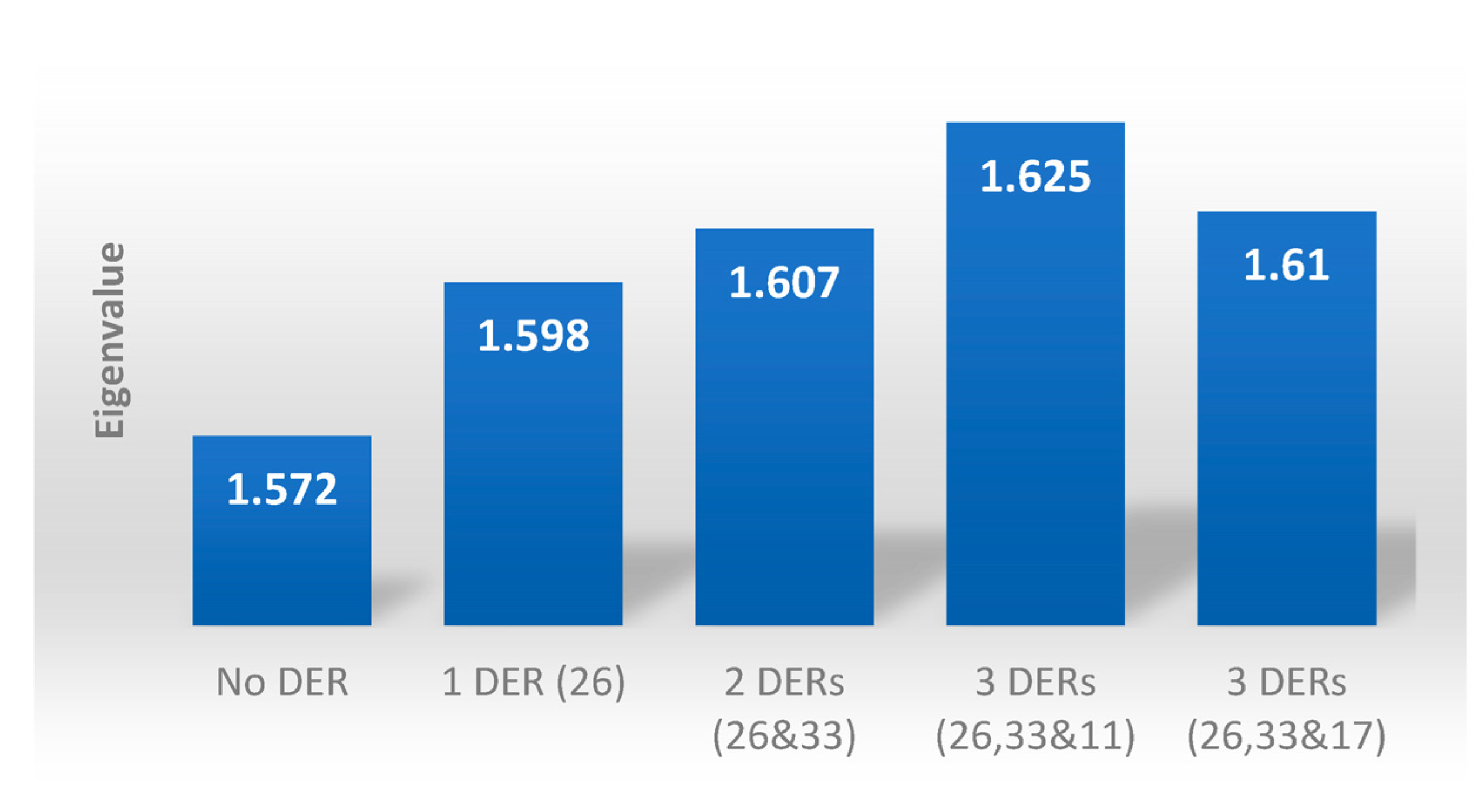
As eigenvalue assessment () is one of the most efficient techniques to evaluate static voltage stability analysis, is utilized to carry out efficient comparison of the DER location attained by the proposed hybrid method and the CPF. As can be perceived in Figure 14, the of the system with the CPF is only 1.610, whereas the with the proposed hybrid method is 1.618, which is larger than the CPF method eigenvalue. This informs that the proposed hybrid approach is rather more efficient than the CPF technique in resolving placement of DER.
Moreover, DER placement based on the proposed hybrid technique results in the largest losses reduction, with 42.25% and 44.59% for and , respectively. However, by using the CPF approach with three DERs at buses 26, 33, and 17, the reduction in losses is not as much as the losses reduction with DERs at buses 26, 33, and 11, where the third DER is placed at bus 17; the losses decline a little below the network losses reduction for the proposed approach. The with CPF is 36.36% and is 41.29%. Table 4 clarifies the and if DERs are placed at particular locations.
6. Conclusions
Appropriate allocation of DERs is essential to exploit DER advantages. This manuscript recommends a novel technique based on two analytical voltage stability analysis approaches, modified modal analysis and continuation power flow (MMA–CPF). The aim of this work is to attain the most stable system, the lowest losses, and the highest system eigenvalue. To assess the efficiency of the developed technique, this work also examines the performance of the system if DER units are sited at the least sensitive and average APF/TVS values buses.
The outcomes of implementing this approach to the modified 34-bus RDN elucidate the efficiency of this technique regarding optimum allocation of DERs. When the DER units are placed according to the proposed hybrid technique (buses 26, 33, and 11), it resulted in the largest losses reduction, with 42.25% for and 44.59% for . The reduction in losses with the comparative method, the CPF approach (buses 26, 22, and 17), is not as much as the losses reduction for DERs placement based on the proposed method, in which the with CPF is 36.36% and is 41.29%. If three DERs are located at buses with low APF/TVS values (buses 1, 2, and 12), the power losses reduction is very insignificant, with of only 4.44% and of 8.88%. Similarly, when three DER units are sited at buses with average values of APF/TVS (buses 1, 15, and 29), the losses reduction is quite low, with the being 7.06% and the 14.27%.
It was proven in this paper that an appropriate DER site is very crucial to maximize the advantages of DER. Proper DER allocation can enhance the voltage profile substantially and reduce network losses significantly. The outcomes demonstrate the robustness of the APF/TVS in deciding optimum placement for DER to improve voltage stability, reduce losses, and also increase the eigenvalue.
Author Contributions
Conceptualization, A.A.; methodology, A.A.; software, A.A. and M.B.N.; validation, A.A. and M.B.N.; formal analysis, A.A. and M.B.N.; investigation, A.A.; resources, A.A. and M.B.N.; data curation, A.A.; writing—original draft preparation, A.A.; writing—review and editing, A.A. and M.B.N.; visualization, A.A.; supervision, M.B.N.; project administration, A.A.; funding acquisition, M.B.N. All authors have read and agreed to the published version of the manuscript.
Funding
This research received no external funding.
Data Availability Statement
The data used in this study are available from the authors upon reasonable request.
Conflicts of Interest
The authors declare no conflict of interest.
Nomenclature
| APF | Active Participation Factor |
| TVS | Tangent Vector Sensitivity |
| RDN | Radial Distribution Network |
| DG | Distributed Generation |
| DER | Distributed Energy Resources |
| MMA | Modified Modal Analysis |
| CPF | Continuation Power Flow |
| MMA–CPF | Modified Modal Analysis–Continuation Power Flow |
| OF | Objective Function |
| Active power variations | |
| Reactive power variations | |
| ∆𝜃 | Voltage angle variations |
| ∆𝑉 | Voltage magnitude variations |
| J | Jacobian Matrix |
| Reduced Modified Jacobian Matrix | |
| Right eigenvector matrix of | |
| Left eigenvector matrix of | |
| Diagonal eigenvalue matrix of | |
| ith eigenvalue of | |
| ith column right eigenvector of | |
| ith row left eigenvector of | |
| Load parameter | |
| Base case active power generation at bus i | |
| Initial active power load at bus i | |
| Injected active power at bus i | |
| Base case reactive power generation at bus i | |
| Initial reactive power load at bus i | |
| Injected reactive power at bus i. | |
| A specified amount of complex power that is selected to offer suitable scaling | |
| Constant assigned for the degree of generation variation at bus i as varies | |
| Constant assigned for the degree of load variation at bus i as varies | |
| Power angle changes at bus i | |
| Vector of generator angle | |
| Vector of the bus voltage magnitude vector | |
| Complex voltages at bus i | |
| Complex voltages at bus j | |
| ijth component of impedance matrix | |
| Active power generation at bus i | |
| Active power generation at bus j | |
| Reactive power injection at bus i | |
| Reactive power injection at bus j | |
| Active power losses at initial conditions without DER integration | |
| Active power losses after integration of DER | |
| Reactive power losses at initial conditions without DER integration | |
| Reactive power losses after integration of DER | |
| Reduction in active power losses | |
| Reduction in reactive power losses | |
| Reduction percentage of active power losses | |
| Reduction percentage of reactive power losses | |
| Voltage stability index, indicating voltage stability improvement after DER placement | |
| The smallest eigenvalue with DER unit(s) | |
| The smallest eigenvalue without any DER unit |
References
- Hung, D.Q.; Mithulananthan, N.; Bansal, R.C. Analytical Expressions for DG Allocation in Primary Distribution Networks. IEEE Trans. Energy Convers. 2010, 25, 814–820. [Google Scholar] [CrossRef]
- Arief, A.; Nappu, M.B.; Rachman, S.M. Photovoltaic Allocation with Tangent Vector Sensitivity. Int. J. Energy Convers. 2020, 8, 71–79. [Google Scholar] [CrossRef]
- Daud, S.; Kadir, A.F.A.; Gan, C.K.; Mohamed, A.; Khatib, T. A comparison of heuristic optimization techniques for optimal placement and sizing of photovoltaic based distributed generation in a distribution system. Solar Energy. 2016, 140, 219–226. [Google Scholar] [CrossRef]
- Arief, A.; Nappu, M.B.; Antamil. Analytical Method for Reactive Power Compensators Allocation. Int. J. Technol. 2018, 9, 602–612. [Google Scholar] [CrossRef]
- Sirjani, R.; Rezaee Jordehi, A. Optimal placement and sizing of distribution static compensator (D-STATCOM) in electric distribution networks: A review. Renew. Sust. Energ. Rev. 2017, 77, 688–694. [Google Scholar] [CrossRef]
- Arief, A.; Dong, Z.; Nappu, M.B.; Gallagher, M. Under voltage load shedding in power systems with wind turbine-driven doubly fed induction generators. Electr. Power Syst. Res. 2013, 96, 91–100. [Google Scholar] [CrossRef]
- Swaminathan, D.; Rajagopalan, A. Optimized Network Reconfiguration with Integrated Generation Using Tangent Golden Flower Algorithm. Energies 2022, 15, 8158. [Google Scholar] [CrossRef]
- Ramshanker, A.; Isaac, J.R.; Jeyeraj, B.E.; Swaminathan, J.; Kuppan, R. Optimal DG Placement in Power Systems Using a Modified Flower Pollination Algorithm. Energies 2022, 15, 8516. [Google Scholar] [CrossRef]
- Atwa, Y.M.; El-Saadany, E.F. Reliability Evaluation for Distribution System With Renewable Distributed Generation During Islanded Mode of Operation. IEEE Trans. Power Syst. 2009, 24, 572–581. [Google Scholar] [CrossRef]
- Kumar, M.; Soomro, A.M.; Uddin, W.; Kumar, L. Optimal Multi-Objective Placement and Sizing of Distributed Generation in Distribution System: A Comprehensive Review. Energies 2022, 15, 7850. [Google Scholar] [CrossRef]
- Barik, S.; Das, D. A novel Q−PQV bus pair method of biomass DGs placement in distribution networks to maintain the voltage of remotely located buses. Energy 2020, 194, 116880. [Google Scholar] [CrossRef]
- Esmaili, M.; Firozjaee, E.C.; Shayanfar, H.A. Optimal placement of distributed generations considering voltage stability and power losses with observing voltage-related constraints. Appl. Energy. 2014, 113, 1252–1260. [Google Scholar] [CrossRef]
- Aman, M.M.; Jasmon, G.B.; Mokhlis, H.; Bakar, A.H.A. Optimal placement and sizing of a DG based on a new power stability index and line losses. Int. J. Electr. Power Energy Syst. 2012, 43, 1296–1304. [Google Scholar] [CrossRef]
- Ishak, R.; Mohamed, A.; Abdalla, A.N.; Che Wanik, M.Z. Optimal placement and sizing of distributed generators based on a novel MPSI index. Int. J. Electr. Power Energy Syst. 2014, 60, 389–398. [Google Scholar] [CrossRef]
- Al Abri, R.S.; El-Saadany, E.F.; Atwa, Y.M. Optimal Placement and Sizing Method to Improve the Voltage Stability Margin in a Distribution System Using Distributed Generation. IEEE Trans. Power Syst. 2013, 28, 326–334. [Google Scholar] [CrossRef]
- Soo-Hyoung, L.; Jung-Wook, P. Selection of Optimal Location and Size of Multiple Distributed Generations by Using Kalman Filter Algorithm. IEEE Trans. Power Syst. 2009, 24, 1393–1400. [Google Scholar] [CrossRef]
- Acharya, N.; Mahat, P.; Mithulananthan, N. An Analytical Approach for DG Allocation in Primary Distribution Network. Int. J. Electr. Power Energy Syst. 2006, 28, 669–678. [Google Scholar] [CrossRef]
- Willis, H.L. Analytical Methods and Rules of Thumb for Modeling DG-Distribution Interaction. In Proceeding of the IEEE Power Engineering Society Summer Meeting, Seattle, WA, USA, 16–20 July 2000. [Google Scholar]
- Hedayati, H.; Nabaviniaki, S.A.; Akbarimajd, A. A Method for Placement of DG Units in Distribution Networks. IEEE Trans. Power Deliv. 2008, 23, 1620–1628. [Google Scholar] [CrossRef]
- Rao, R.S.; Ravindra, K.; Satish, K.; Narasimham, S.V.L. Power Loss Minimization in Distribution System Using Network Reconfiguration in the Presence of Distributed Generation. IEEE Trans. Power Syst. 2013, 28, 317–325. [Google Scholar] [CrossRef]
- Huy, P.D.; Ramachandaramurthy, V.K.; Yong, J.Y.; Tan, K.M.; Ekanayake, J.B. Optimal placement, sizing and power factor of distributed generation: A comprehensive study spanning from the planning stage to the operation stage. Energy 2020, 195, 117011. [Google Scholar] [CrossRef]
- García-Muñoz, F.; Díaz-González, F.; Corchero, C. A novel algorithm based on the combination of AC-OPF and GA for the optimal sizing and location of DERs into distribution networks. Sustain. Energy Grids Netw. 2021, 27, 100497. [Google Scholar] [CrossRef]
- Mouwafi, M.T.; El-Sehiemy, R.A.; El-Ela, A.A.A. A two-stage method for optimal placement of distributed generation units and capacitors in distribution systems. Appl. Energy. 2022, 307, 118188. [Google Scholar] [CrossRef]
- Roy, N.B.; Das, D. Optimal allocation of active and reactive power of dispatchable distributed generators in a droop controlled islanded microgrid considering renewable generation and load demand uncertainties. Sustain. Energy Grids Netw. 2021, 27, 100482. [Google Scholar] [CrossRef]
- Lingfeng, W.; Singh, C. Reliability-Constrained Optimum Placement of Reclosers and Distributed Generators in Distribution Networks Using an Ant Colony System Algorithm. IEEE Trans. Syst. Man Cybern. Part C Appl. Rev. 2008, 38, 757–764. [Google Scholar]
- Mohamed Imran, A.; Kowsalya, M.; Kothari, D.P. A novel integration technique for optimal network reconfiguration and distributed generation placement in power distribution networks. Int. J. Electr. Power Energy Syst. 2014, 63, 461–472. [Google Scholar] [CrossRef]
- Martín García, J.A.; Gil Mena, A.J. Optimal distributed generation location and size using a modified teaching–learning based optimization algorithm. Int. J. Electr. Power Energy Syst. 2013, 50, 65–75. [Google Scholar] [CrossRef]
- Gao, B.; Morison, G.K.; Kundur, P. Voltage Stability Evaluation Using Modal Analysis. IEEE Trans. Power Syst. 1992, 7, 1529–1542. [Google Scholar] [CrossRef]
- Arief, A. Optimal placement of distributed generations with modified P-V Modal Analysis. In Proceedings of the 2014 Makassar International Conference on Electrical Engineering and Informatics (MICEEI), Makassar, Indonesia, 26–30 November 2014. [Google Scholar]
- Ajjarapu, V.; Christy, C. The Continuation Power Flow: A Tool for Steady State Voltage Stability Analysis. IEEE Trans. Power Syst. 1992, 7, 416–423. [Google Scholar] [CrossRef]
- Arief, A.; Nappu, M.B. DG placement and size with continuation power flow method. In Proceedings of the 2015 International Conference on Electrical Engineering and Informatics (ICEEI), Bali, Indonesia, 10–11 August 2015. [Google Scholar]
- Kothari, D.P.; Dhillon, J.S. Power System Optimization; Prentice-Hall of India: New Delhi, India, 2004. [Google Scholar]
Figure 1.
The hybrid MMA–CPF DER allocation approach flowchart.

Figure 2.
IEEE 34-bus distribution network test system [19].
Figure 2.
IEEE 34-bus distribution network test system [19].
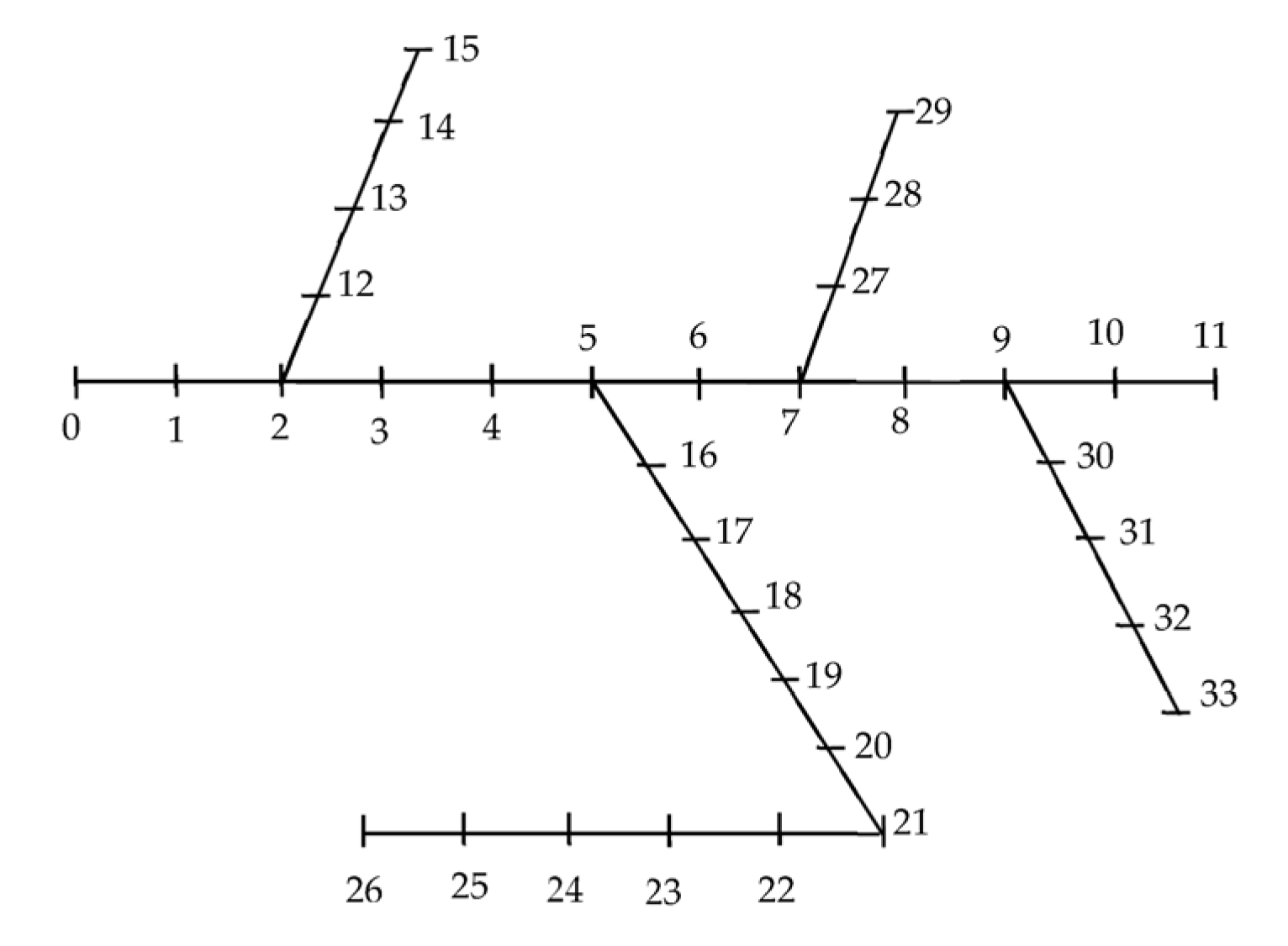
Figure 3.
The APF and TVS for determining the first DER location.
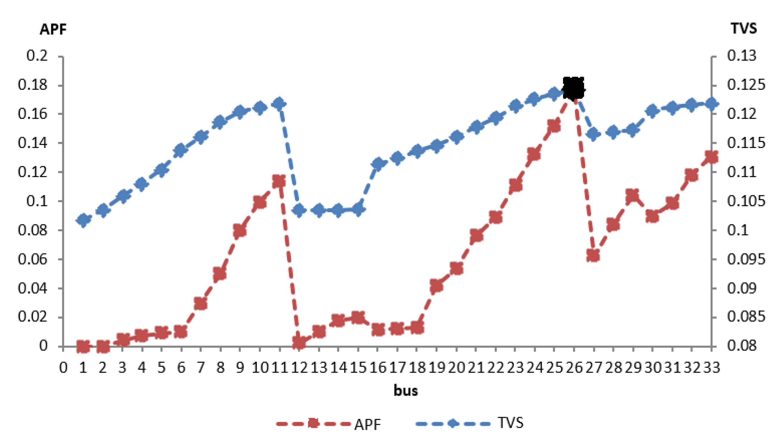
Figure 4.
The APF and TVS for determining the second DER location.
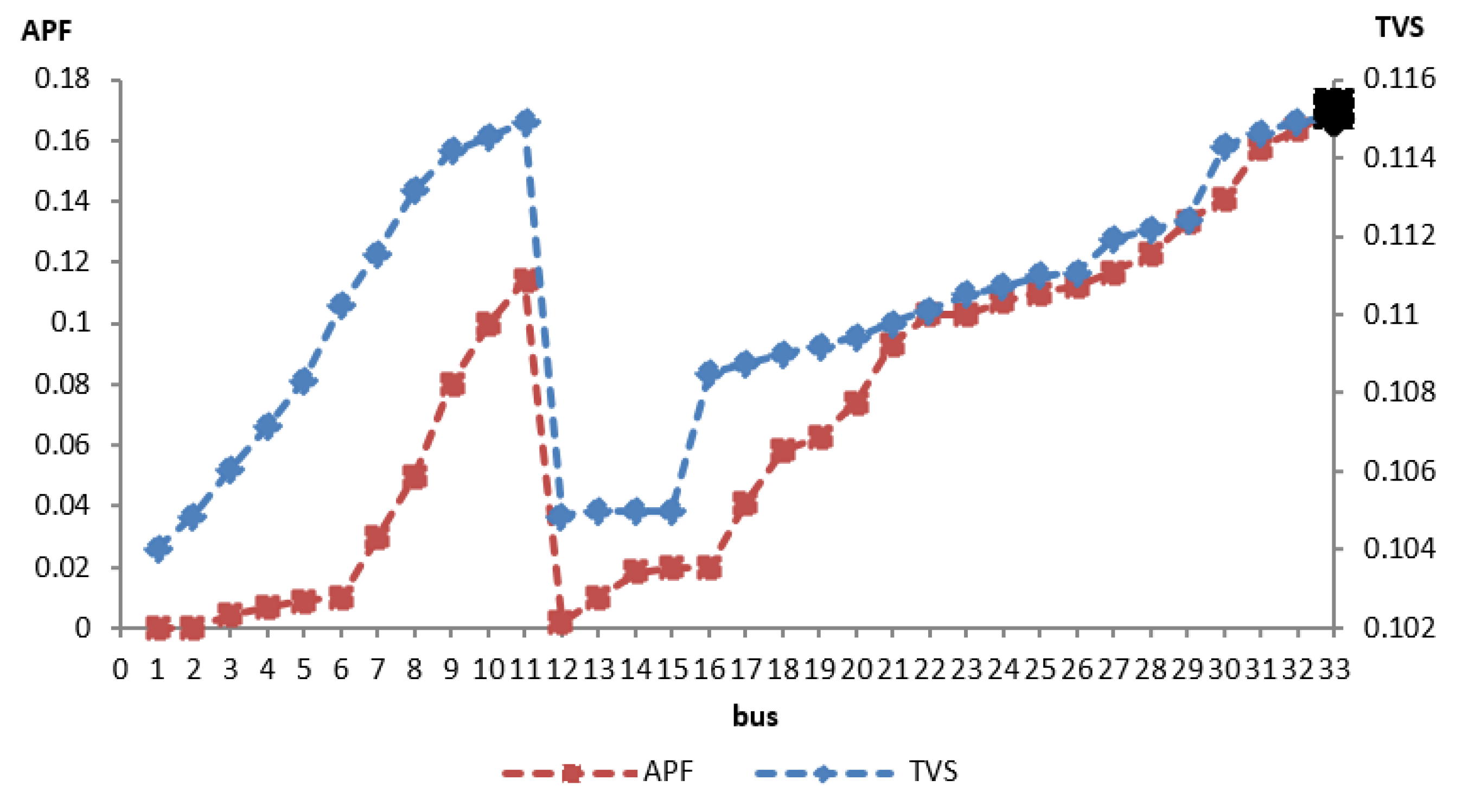
Figure 5.
The APF and TVS for determining the third DER location.
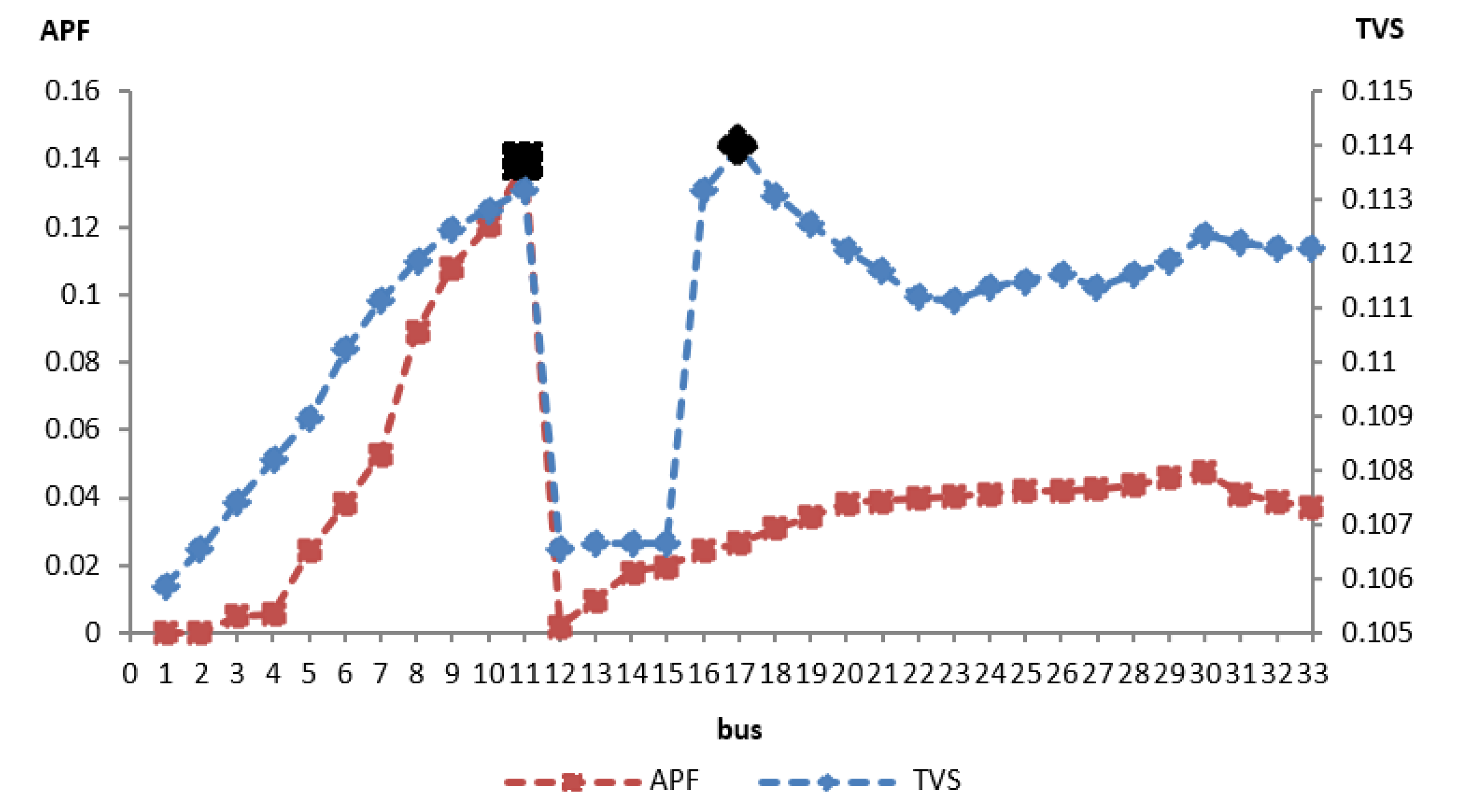
Figure 6.
Objective function (OF) to determine the third DER location.
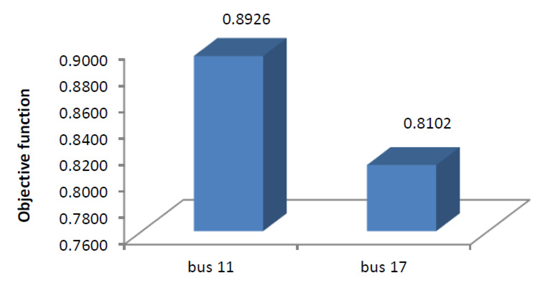
Figure 7.
Voltage profile improvement with DER units placement.
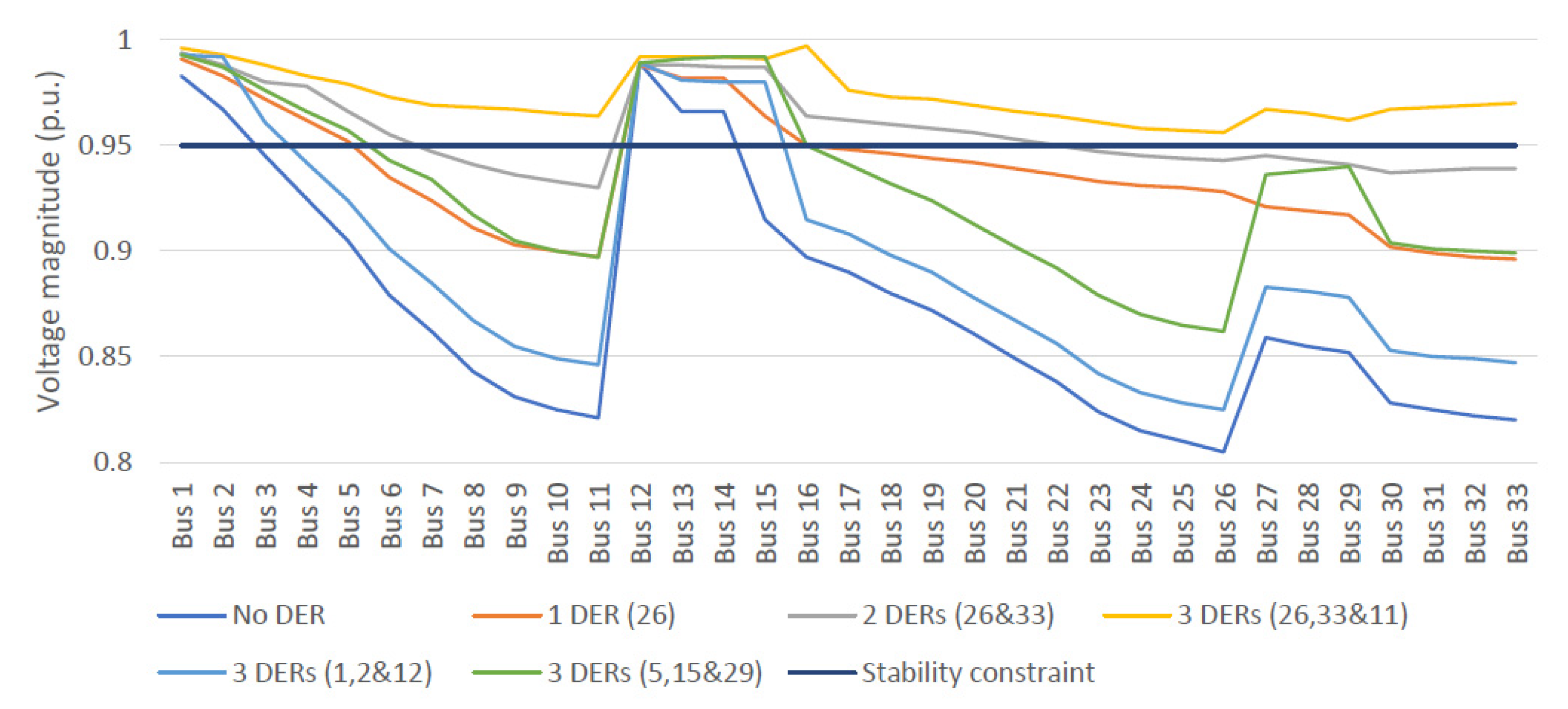
Figure 8.
The system’s smallest eigenvalue comparison.
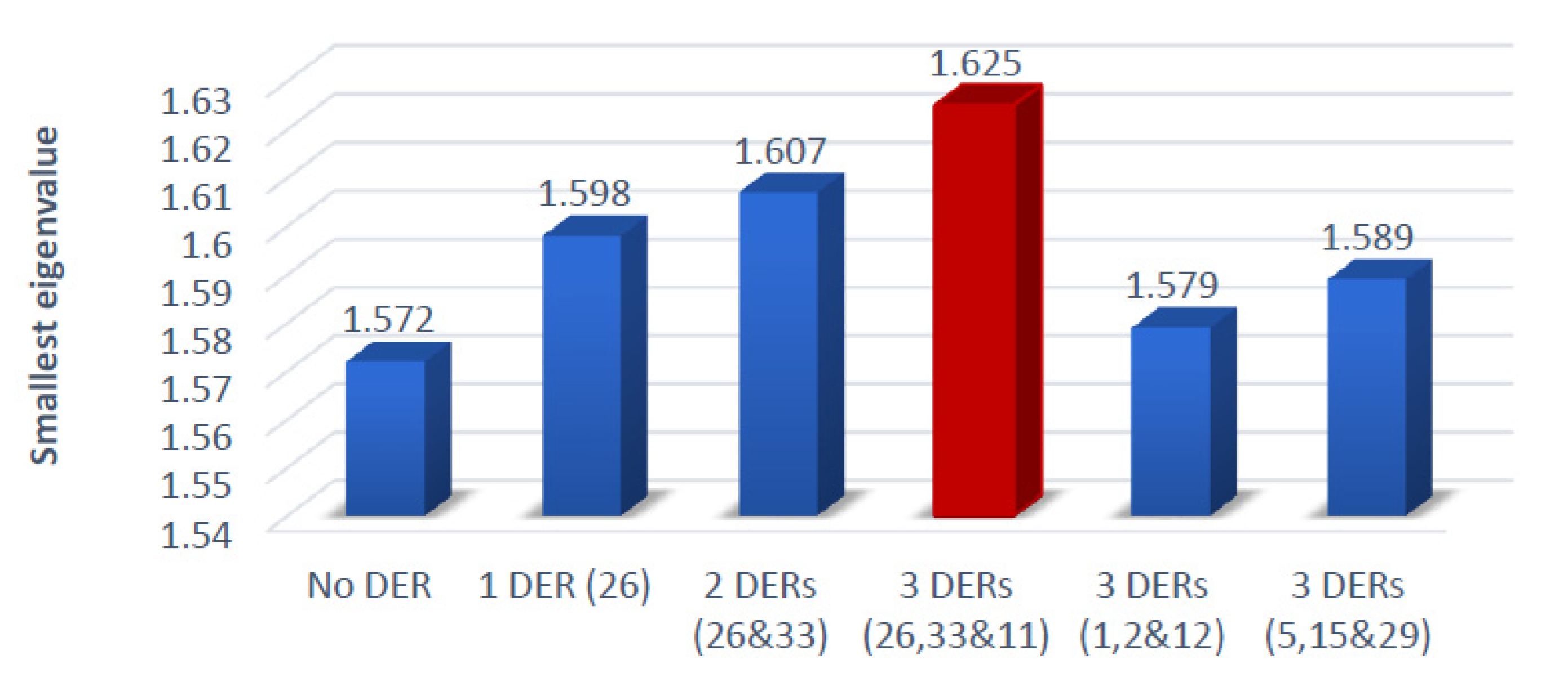
Figure 9.
Comparison of system losses after DER units placement.
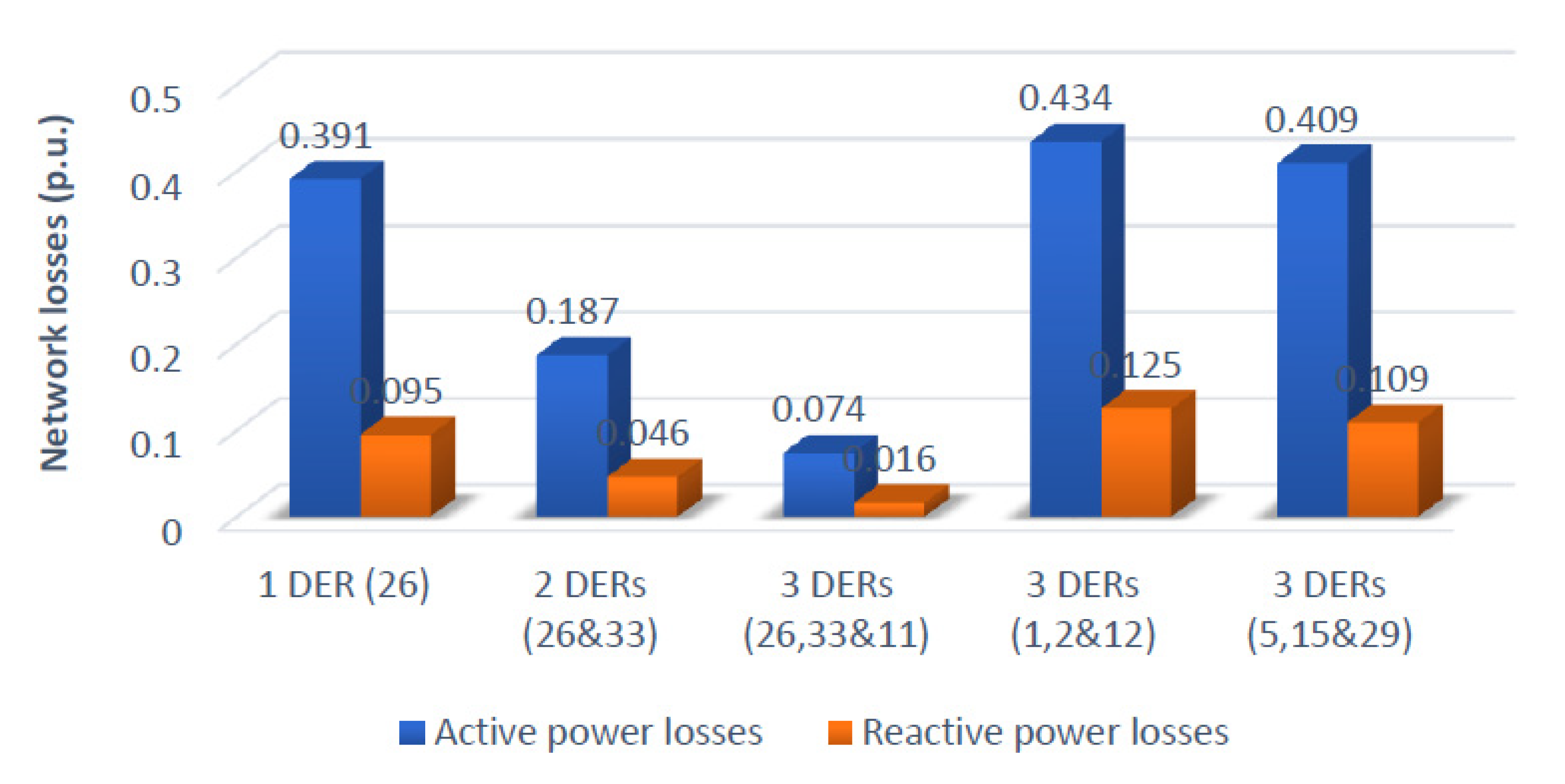
Figure 10.
Comparison of voltage profile.
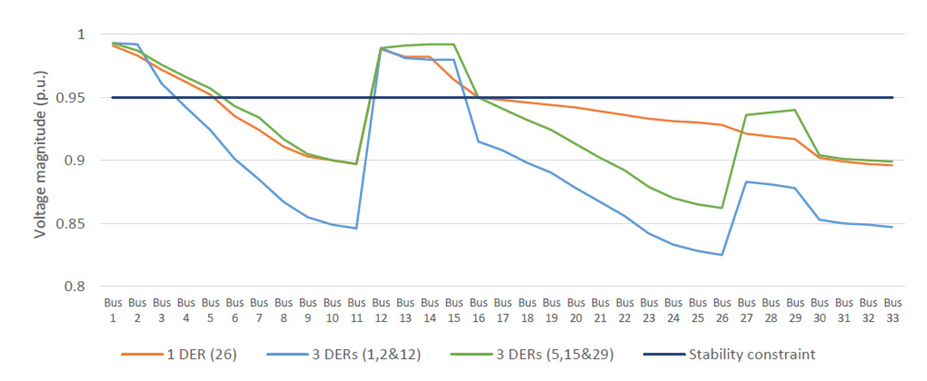
Figure 11.
System eigenvalue comparison.
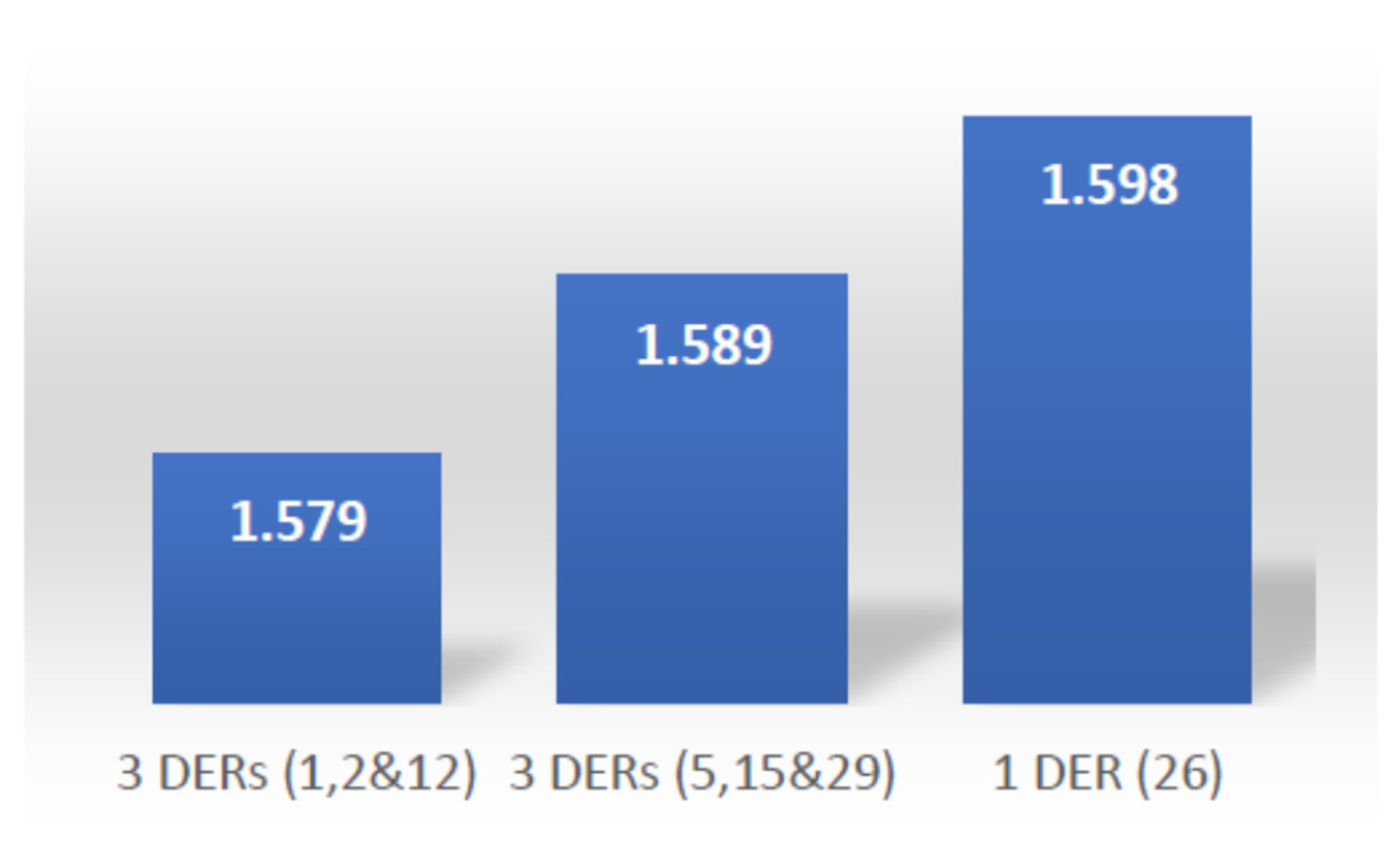
Figure 12.
Losses comparison.
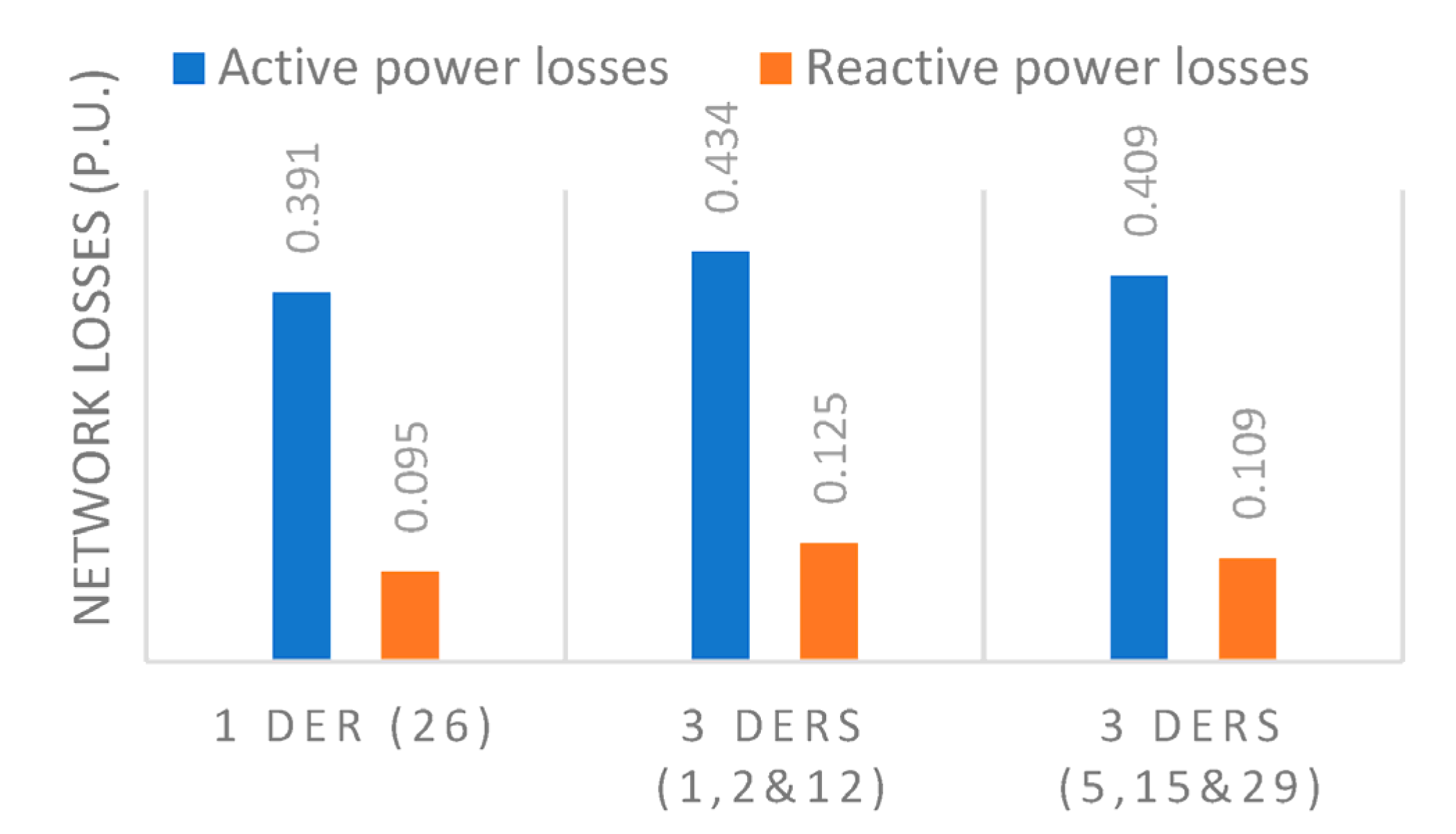
Figure 13.
Voltage magnitude after DER integration with the CPF method and the proposed hybrid method.
Figure 13.
Voltage magnitude after DER integration with the CPF method and the proposed hybrid method.
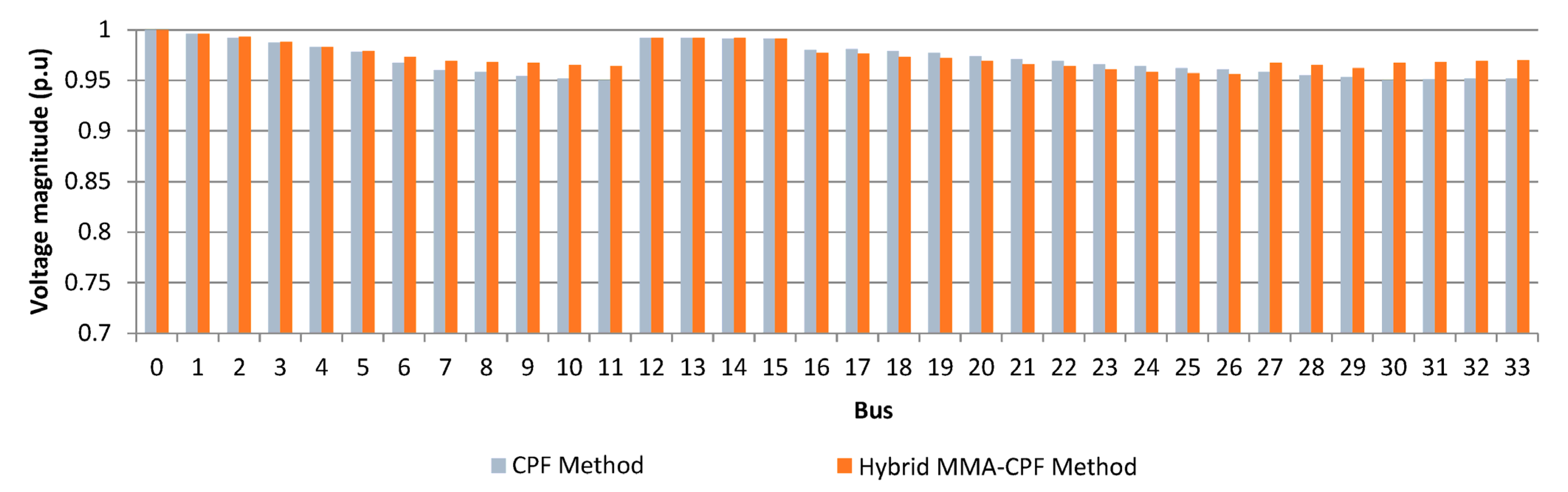
Figure 14.
System eigenvalues with the CPF approach and the proposed method.

Table 1.
Summary of the results of the highest APF, TVS, and OF calculations to determine the DER location.
Table 1.
Summary of the results of the highest APF, TVS, and OF calculations to determine the DER location.
| Iteration | Highest APF | Highest TVS | Highest OF | DER Location |
|---|---|---|---|---|
| 1 | 26 | 26 | - | 26 |
| 2 | 33 | 33 | - | 33 |
| 3 | 11 | 17 | 11 | 11 |
Table 2.
Results comparison in terms of the system smallest eigenvalue, and network losses reduction percentage.
Table 2.
Results comparison in terms of the system smallest eigenvalue, and network losses reduction percentage.
| High Values of APF/TVS (Recommended) | Small Values of APF/TVS | Average Values of APF/TVS | |
|---|---|---|---|
| DER Locations | 26, 33, and 11 | 1, 2, and 12 | 5, 15, and 29 |
| 1.625 | 1.579 | 1.589 | |
| 42.25 | 4.44 | 7.06 | |
| 44.59 | 8.88 | 14.27 |
Table 3.
DER locations.
| Iteration | CPF Method [19] | Proposed Method Hybrid MMA–CPF |
|---|---|---|
| 1 | 26 | 26 |
| 2 | 33 | 33 |
| 3 | 17 | 11 |
Table 4.
Results comparison.
| DER Placement | Approach | VSI (%) | OF | |||
|---|---|---|---|---|---|---|
| 26, 33, and 17 | CPF [19] | 1.610 | 36.36 | 41.29 | 2.430335 | 80.08033 |
| 26, 33, and 11 | MMA–CPF | 1.618 | 42.25 | 44.59 | 2.939305 | 89.77931 |
| 26 and 33 | Both | 1.6067 | 30.34 | 35.33 | 2.220384 | 67.89038 |
| 26 | Both | 1.5988 | 8.87 | 18.97 | 1.717776 | 29.55778 |
Disclaimer/Publisher’s Note: The statements, opinions and data contained in all publications are solely those of the individual author(s) and contributor(s) and not of MDPI and/or the editor(s). MDPI and/or the editor(s) disclaim responsibility for any injury to people or property resulting from any ideas, methods, instructions or products referred to in the content. |
© 2023 by the authors. Licensee MDPI, Basel, Switzerland. This article is an open access article distributed under the terms and conditions of the Creative Commons Attribution (CC BY) license (https://creativecommons.org/licenses/by/4.0/).
Share and Cite
MDPI and ACS Style
Arief, A.; Nappu, M.B. Novel Hybrid Modified Modal Analysis and Continuation Power Flow Method for Unity Power Factor DER Placement. Energies 2023, 16, 1698. https://doi.org/10.3390/en16041698
AMA Style
Arief A, Nappu MB. Novel Hybrid Modified Modal Analysis and Continuation Power Flow Method for Unity Power Factor DER Placement. Energies. 2023; 16(4):1698. https://doi.org/10.3390/en16041698
Chicago/Turabian StyleArief, Ardiaty, and Muhammad Bachtiar Nappu. 2023. "Novel Hybrid Modified Modal Analysis and Continuation Power Flow Method for Unity Power Factor DER Placement" Energies 16, no. 4: 1698. https://doi.org/10.3390/en16041698
Note that from the first issue of 2016, this journal uses article numbers instead of page numbers. See further details here.