
A Review of Drive Cycles for Electrochemical Propulsion
by
 , and
, and
Jia Di Yang
1,2,
Jason Millichamp
1,2,
Theo Suter
1,2,
Paul R. Shearing
1,3,
Dan J. L. Brett
1,2,3 and
James B. Robinson
1,2,3,* 1
Electrochemical Innovation Lab, Department of Chemical Engineering, University College London, London WC1E 7JE, UK
2
Advanced Propulsion Lab, UCL East, University College London, London E15 2JE, UK
3
The Faraday Institution, Quad One, Becquerel Avenue, Harwell Science and Innovation Campus, Didcot OX11 0RA, UK
*
Author to whom correspondence should be addressed.
Energies 2023, 16(18), 6552; https://doi.org/10.3390/en16186552
Submission received: 18 August 2023
/
Revised: 8 September 2023
/
Accepted: 9 September 2023
/
Published: 12 September 2023
(This article belongs to the Topic Advanced Energy and Propulsion Technology for Electric and Intelligent Transportation)
Abstract
:Automotive drive cycles have existed since the 1960s. They started as requirements as being solely used for emissions testing. During the past decade, they became popular with scientists and researchers in the testing of electrochemical vehicles and power devices. They help simulate realistic driving scenarios anywhere from system to component-level design. This paper aims to discuss the complete history of these drive cycles and their validity when used in an electrochemical propulsion scenario, namely with the use of proton exchange membrane fuel cells (PEMFC) and lithium-ion batteries. The differences between two categories of drive cycles, modal and transient, were compared; and further discussion was provided on why electrochemical vehicles need to be designed and engineered with transient drive cycles instead of modal. Road-going passenger vehicles are the main focus of this piece. Similarities and differences between aviation and marine drive cycles are briefly mentioned and compared and contrasted with road cycles. The construction of drive cycles and how they can be transformed into a ‘power cycle’ for electrochemical device sizing purposes for electrochemical vehicles are outlined; in addition, how one can use power cycles to size electrochemical vehicles of various vehicle architectures are suggested, with detailed explanations and comparisons of these architectures. A concern with using conventional drive cycles for electrochemical vehicles is that these types of vehicles behave differently compared to combustion-powered vehicles, due to the use of electrical motors rather than internal combustion engines, causing different vehicle behaviours and dynamics. The challenges, concerns, and validity of utilising ‘general use’ drive cycles for electrochemical purposes are discussed and critiqued.
1. Introduction
Drive cycles are standardised speed vs. time data profiles used by automotive manufacturers, testers, and researchers for fuel consumption, emissions, and durability testing and validation [1]. Over the years, they have changed from being used solely for emissions and dynamometer testing in internal combustion engine (ICE) applications to also acting as inputs for vehicle simulations, parameterising, and powertrain component sizing [1]. In a review paper published in 2002 by Esteves-Booth et al., it mentioned simulation and estimation capabilities of certain drive cycles, and how drive cycles provide more than just emissions testing [2]. This paper was over two decades ago, when drive cycles were starting to become more popular for simulations rather than solely for emissions testing. Over the past decade, battery electric- and fuel cell-powered vehicles have initially attracted more interest and increasingly a higher market share due to a range of legislative and environmental factors. These vehicles have the potential to reduce and, indeed, remove, combustion emissions, including CO2 and NOx, resulting in improved air quality and mitigated environmental impact from personal transportation. When studying the performance of these vehicles or energy sources, drive cycles are a crucial tool to simulate realistic driving. These cycles are used by systems designers and researchers for activities as diverse as cell-level degradation studies to pack-level component sizing.
No global standard exists for drive cycles, although certain drive cycles, such as the Worldwide Harmonised Light Vehicles Test Procedure (WLTP) and Federal Test Procedure (FTP), are extensively employed and becoming mandated to be used by automotive manufacturers upon the release of a new vehicle. Some countries and regions have also implemented their own specific legislative drive cycles, such as The New European Drive Cycle (NEDC) or China Automotive Test Cycle (CATC), while others use a jointly produced worldwide drive cycle [3]. However, all drive cycles have their limitations and are not universally applicable across different vehicle powertrain architectures (ICE, EV, and hybrid), vehicle size classifications, and natures of application. Other limitations have been identified, including not accurately representing real-world driving behaviours, which can include significant differences in energy usage between drive cycles using similar dynamics, locations having different driving dynamics than others, and region-specific driving styles and needs [1,4,5]. For example, Son et al. conducted a driving comparison study between driving in the United Kingdom (UK) and South Korea using a combustion-powered vehicle (CV). The driving survey was conducted based on similar road conditions in the UK and North Korea, with the UK being slightly higher in driving distance. It was found that the vehicles driven in the UK have resulted in a much higher fuel economy; the vehicle used in the UK had a fuel efficiency of 19.52 km L−1, while the vehicle used in South Korea had a fuel efficiency of 8.66 km L−1 [6]. This was due to different driver characteristics, road environments, and traffic flow between the two regions. This suggests that if a UK-based drive cycle were to be used to design and estimate the range of a vehicle for the South Korean market, the result would be skewed.
Drive cycles can be divided into two categories: modal and transient. Transient drive cycles are usually collected based on real driving data while modal cycles are not. This categorisation will be further explained in Section 2.2. The introduction of drive cycles in different regions of the world has evolved as summarised in Figure 1. In Japan, the first-ever legislative drive cycle, 4-Mode, was introduced in 1966 [7,8]. Thirty-nine years later, this was superseded by the JC08 cycle in 2005 [9]. In the United States, the California 7-Mode drive cycle was established in 1968 [7,8]. The latter cycle was created based on Los Angles Street conditions and was used as a national drive cycle [7,8]. The EPA Federal Test Procedure drive cycle was introduced as a legislative test procedure for passenger cars in 1972, hence the naming classification (FTP-72) [7,8]. FTP-72 later became FTP-75 in 1975 [9]. These two cycles were established with the aim of streamlining the implementation of the 1978 gas guzzler tax, which serves as a deterrent for manufacturing vehicles with a low fuel efficiency [7,8,9,10,11]. In 1970, European countries started with a legislative modal cycle, UN-ECE Regulation Number 15 (ECE-15), which later became a part of the New European Drive Cycle (NEDC); this was later replaced by a cycle known as the Worldwide Harmonised Light Vehicle Test Procedure (WLTP) cycle in 2017 [3]. In 2019, China introduced its transient drive cycle, China Automotive Test Cycles (CATC), to reflect the country’s unique driving dynamics due to extreme congestion resulting from overpopulation [12]. A detailed historical discussion of these drive cycles is covered in Section 2.3. None of the drive cycles in the timeline was built purely for electric vehicles, but as ‘general use’ cycles. The electric motor is a major component that makes electric vehicles different from CV driving. Electric vehicles have instant torque from a standstill and produce a speed and acceleration curve different from those of CVs, which should be represented in a drive cycle. Protocols already exist in converting conventional-use drive cycles for electrochemical bench testing; for example, Fuel Cell and Hydrogen Joint Undertaking (FCH) has a current control-based NEDC drive cycle for fuel cell bench testing [13]. However, NEDC was a modal drive cycle introduced earlier in the 1980s [14], when electrochemical vehicles were far less utilised and researched compared to today. In addition, NEDC was not collected from real-life driving data; instead, it was a dynamometer testing cycle better suited for emissions testing rather than vehicle engineering or simulation. Using a transient drive cycle that mimics real-life driving scenarios and actual vehicle behaviour is crucial for the proper design and accurate range estimation of electrochemical vehicles, which is covered in Section 2.8. Jeong et al. simulated electric vehicle driving based on conventional drive cycles and concluded that the cycles do not account for the higher acceleration capabilities of electric vehicles [15]. In addition, the importance of developing ‘electric-only’ drive cycles was emphasised. An electric vehicle transient drive cycle can be collected using techniques such as the micro-trip clustering technique combined with a CANBUS datalogger. Some electric drive cycle collections have been done in the past, such as in a study conducted by Peng et al. for developing a hybrid electric bus cycle in Zhengzhou, China using the Markov chain method [16]. However, none are legislated for widespread use and tend to be city, research facility, or academic institution dependent. The lack of electric drive cycles is a legislative problem rather than an engineering problem, as collecting one is straightforward but requires organisation, data acquisition, and manpower. As we enter the age of electrochemical propulsion, legislated and dedicated region-specific electric vehicle drive cycles are crucial for the accurate representation of these vehicles.
There have been review papers regarding drive cycles in the previous literature, but very few recent ones; none have gone into depth about the history of the cycles and their adaptability to electrochemical vehicles of the current decade. Esteves-Booth et al. published a review paper in 2002, which reviewed developments in drive cycles and broke them down into emission factor, speed, and modal models [2]. Emission factor models only correspond to one type of vehicle and driving route and are not representative of other types of vehicles, such as electrochemical vehicles. Average speed models rely on emission functions and are mainly used for emissions testing instead of vehicle or device simulations. Modal cycles are described in the paper as the most realistic compared to real-world driving. However, this paper was published in 2002, when very few countries had introduced a legislative transient cycle; only the United States had a transient cycle at the time, FTP-72. Samuel et al. emphasised, in their review paper, that transient cycles should be used for accurate emissions testing and estimation of vehicles [17]. Again, this paper was published in 2002, when electrochemical vehicles were less popularised. In a more recent paper, Tong et al. developed a drive cycle for an electric bus operating in Hong Kong and compared characteristics, such as velocity and acceleration trends of the drive cycle, to those of other bus cycles [18]. Similar discussions and comparisons of these characteristics can be found in this paper in Section 2.4 and Section 2.5 for passenger cars.
2. Review
2.1. Breakdown of Topics
The paper first explains the differences between two types of drive cycles: modal and transient and then dives into a complete historical overview of legislative drive cycles, divided by countries or regions. Why these cycles were formulated and how they have changed over time are discussed. In addition, important characteristics, such as top and average speeds and accelerations, idle percentages, and durations, are discussed. If possible, the discussed drive cycles are graphed in terms of standard speed vs. time data. Most legislated drive cycle data can be found and extracted from MATLAB. It should be pointed out, however, some of the newer drive cycle data, such as CATC, were unable to be graphed by the authors due to the lack of available information. For road vehicles, only passenger car cycles are included for the scope of this Review. HGV (heavy goods vehicle) drive cycles are mentioned but not discussed in depth. Some of the older drive cycles, such as ECE-15, were recorded in treaties and legal document archives dating back to the 1970s. Aviation and marine cycles are also mentioned, acting as supplementary discussion and comparison to the road vehicle cycles. The aforementioned topics are covered in Section 2.2, Section 2.3, Section 2.4. Section 2.5 discusses a commonly used method of drive cycle collection of formulation: the micro-trip clustering technique. All the aforementioned sections discuss topics within the speed domain, power cycles, or duty profiles and are excluded. Section 2.6, Section 2.7, Section 2.8, Section 2.9 discuss topics related more to the power domain, particularly the use of duty profiles or power cycles. The section starts with electrochemical cell-level bench testing (Section 2.6) and scales up to vehicular scenarios (Section 2.7, Section 2.8, Section 2.9). A summary on how power cycles can be important for electrochemical device sizing and the need for more standardised transient bench testing cycles is included in Section 2.6. Section 2.7 discusses a method that can be used to convert speed vs. time drive cycle profiles to power vs. time power cycles. Section 2.8 expands further on possible usages for the power cycles obtained, in terms of vehicle sizing for different electric and hybrid vehicle architectures. The vehicle architectures are briefly explained in ICE-battery hybrid vehicle terms, with suggestions on how net-zero hybridisation solutions can be implemented between electrochemical devices (no ICE). The architectures are explained from the least electrified to the most electrified. Section 2.9 addresses the complications and limitations of using pre-existing ‘general-use’ drive cycles for electrochemical vehicles and addresses the importance of having propulsion-specific drive cycles when designing vehicles. Previous works of other authors who have used conventional drive cycles on electrochemical vehicle testing are surveyed and discussed.
2.2. Drive Cycle Classification
Drive cycles can be divided into two categories: modal and transient [4,5]. Modal drive cycles, such as the New European Drive Cycle (NEDC), are designed for specific regulation testing [1]. Modal drive cycles tend to have sections of linear acceleration and constant velocity, as shown in the NEDC example in Figure 2, and do not accurately depict realistic driving behaviours [1,4,5]. Transient cycles, on the other hand, are collected from real driving data, typically using a global positioning datalogger (GPD) or CAN-BUS readers, such as Advanced Vehicle Location (AVL) [19], OXTS inertial+ [16], or Launch Tech Diagnostic Tools; these tools help determine vehicle location, gradient, and speed data via GPS and CAN messages from a vehicle [1,4,5,20]. Figure 2 is a speed vs. time graphical comparison between a modal (NEDC) and transient (WLTP Class 3) drive cycle. As seen in the figure, modal drive cycles appear less varying, while transient cycles appear more random. NEDC contains four repetitions of the same profile of the ECE-15 drive cycle, which represents urban driving, and one repetition of the Extra-Urban Driving Cycle (EUDC), which represents highway driving. In contrast, the WLTP cycle is divided into four sections: low, medium, high, and extra high. These sections have increasing average speeds to represent driving on distinct types of roads and under different traffic conditions. Low represents congested traffic, medium and high represent more free-flowing urban traffic, and extra-high represents highway driving. A more thorough explanation of NEDC and WLTP Class 3 can be found in Section 2.3.1 and Section 2.3.5.
2.3. Overview and History of Legislative Drive Cycles Sorted by Region and Vehicle Type
2.3.1. European Drive Cycles
UN-ECE Regulation Number 15 was introduced in Europe, in 1970, to simulate urban driving [11,21]. This modal drive cycle later became a part of the NEDC, which was introduced in 1980 [14,22]. There was legislation regarding vehicle emissions before 1970, in the form of the Agreement of 20 March 1958, which concerned the adoption of uniform conditions of approval and reciprocal recognition of approval for motor vehicle equipment and parts, but no actual drive cycle was introduced [21]. This agreement, however, led to the introduction of UN-ECE Regulation Number 15 in 1970 [21]. The UN-ECE Regulation Number 15 Test consists of three separate parts: Type-I, pollutant emissions testing for speeds up to 50 km h−1; Type-II, carbon-monoxide emissions testing during idling; and Type-III, crank-case emissions testing [11,21]. The regulation was an attempt to evaluate the emissions of urban driving and was later adopted as a component of the New European Drive Cycle (NEDC).
The NEDC for passenger cars was introduced in 1980, and this was mandated in most of Europe. This NEDC represented urban driving only and included four repetitions of the pre-existing ECE-15 cycle (Type I test of UN-ECE Regulation Number 15), for a total duration of 780 s [14]. Although the Type-I test of UN-ECE Regulation 15 that was used during the 1970s consisted of repeating the ECE-15 cycle four times, it did not have the official cycle name of NEDC until 1980 [22]. In 1992, a new section, named the Extra Urban Drive Cycle (EUDC), was added to the NEDC to account for non-urban speeds, such as during highway driving. The EUDC has an average and top speed of 62.59 km h−1 and 120 km h−1, respectively [14]. With the new addition, the average and top speeds of NEDC became 33 km h−1 and 120 km h−1, respectively [14]. After the addition of EUDC, NEDC remained unchanged and stayed as a European legislative cycle; the WLTP was mandated in 2017. The final version of NEDC is shown in Figure 2. Like most modal drive cycles, the NEDC has been criticised for its failure to represent real-world driving behaviour [4]. The drive cycle has an abundance of constant speed travel and idling durations, and this has made it difficult to estimate some vehicle parameters, such as fuel economy and range [4,12,23].
2.3.2. American Drive Cycles
The US first adopted a modal drive cycle, named ‘California 7-Mode’, in 1968 [7,8]. This drive cycle was mainly based off-road, in Los Angeles, but was used to represent US national driving [7,8]. Even though this drive cycle did not become mandated until 1968, early drive cycle development had been carried out since the 1950s, with the Los Angeles County Air Pollution Control District Laboratory surveying a single Los Angeles route [7,8]. This survey was later updated and improved, in 1956, by the Automobile Manufacturers Association [7,8]. The drive cycle had a duration of only 137 s, with a maximum and average speed of 80 km h−1 and 41.8 km h−1, respectively. As with all modal cycles, this cycle was criticised for not representing real-world driving, especially during rush hour conditions.
In 1972, the US released the EPA Federal Test Procedure for passenger cars, also referred to as the EPA Urban Dynamometer Driving Schedule (UDDS), or FTP-72, which is shown in Figure 3a [9]. This transient drive cycle was created upon the introduction of the ‘gas guzzler’ tax, which imposed a tax on users with heavy emission vehicles [10]. It has a duration, average speed, and maximum speed of 1372 s, 31.5 km h−1, and 91.3 km h−1, respectively [24]. FTP-72 is divided into two phases: the cold start phase, which accounts for the first 505 s, and the stabilised phase, which accounts for the remaining 867 s [1,24,25,26]. The cold start phase requires the vehicle to be running at an ambient temperature of 20 to 30 °C [25]. FTP-75, shown in Figure 3b, is an extended variant of FTP-72, with the addition of the hot start phase at the end; it is also used in Australia and Sweden, but under different names (Australian Design Rules and Constant Volume Sampler) [1,25]. The hot start phase is a repeat of the cold start transient phase (first 505 s) of FTP-72, except that it is tested under different temperature conditions; specifically, the vehicle is ‘hot soaked’ or kept at a desired operating temperature (‘warmed-up’ temperature for the vehicle) for 540 to 660 s before the commencement of the phase [9,25,27]. FTP-75 has a duration, average speed, and top speed of 1877 s, 34.1 km h−1, and 56.7 km h−1, respectively, when not including the hot soak period [28]. When the hot soak period is included, the overall duration of the test is increased to 2417 to 2537 s [28]. Some vehicle simulation software and programming plugins, such as ADVISOR and MATLAB Simulink Drive Cycle Source blockset, includes the hot soak period as a default when the drive cycle sources or functions are used [27,28], although this can be adjusted according to the simulation needed. Figure 3 shows the aforementioned drive cycles.
In 1996, the US Supplemental Federal Test Procedure (SFTP) cycle was developed as an addition to the pre-existing FTP-75 cycle, in the form of SFTP-US06 and SFTP-SC03, as shown in Figure 3c,d, to account for higher rates of acceleration, higher speeds, and the use of climate-control functions [25,29]. SFTP-US06 was added to account for higher-velocity driving and has a duration of 596 s, with an average speed and maximum speed of 78 km h−1 and 129 km h−1, respectively [25,30]. The SFTP-SC03 incorporated climate-control use [25,31]. the cycle collects data in the form of speed vs. time data but requires that the vehicle be tested with the air conditioning on to measure emissions associated with climate-control function usage [31]. It has a duration, average velocity, and maximum velocity of 596 s, 35 km h−1, and 88 km h−1, respectively [31].
Although US SFTP tests were introduced in 1996, they were not mandated until 2007 [29,32]. Specified climate-control test conditions were administered to newly manufactured light-duty vehicles (LDVs) requiring SFTP-SC03 certification [32]. These conditions simulate hot and cold ambient temperatures, i.e., 35 and −7 °C, respectively [32]. Climate-control systems are turned on to represent realistic driver comfort settings, and the vehicle is run on a dynamometer using the SFTP-SC03 cycle [31,32].
In 2008, a further drive cycle was added to the US EPA tests, namely the Highway Fuel Economy Test Cycle (HWFET) [25]. This cycle was proposed to simulate highway driving and used in synchronisation with the pre-existing city driving cycle, FTP-75, to identify both highway and urban fuel economy ratings [33]. The EPA released the 5-cycle test method in 2008. This consisted of two tests of the FTP-75 cycle, one with the average ambient temperature and one with a cold temperature; the two SFTP tests (SFTP-US06 and SFTP-SC03); and the newly introduced HWFET [25]. The EPA Federal Test Procedure was unchanged after this addition.
2.3.3. Japanese Drive Cycles
Before the first European and United States legislative cycles were introduced, Japan had developed its driving cycle, the 4-Mode, or J4, in 1966 [34]. The 4-Mode is a simple modal cycle, with cruising speed varying from 10 to 70 km h−1 in increments of 10 km h−1 [7]. 4-Mode has a maximum speed of 70 km h−1 [7]. The Japan 10-Mode replaced this drive cycle in 1973 [7]. Similar to ECE-15, the 10-Mode is a longer driving cycle that simulates urban driving only. Just as EUDC was added to ECE-15 to form NEDC, the 10-Mode was later expanded with a separate drive cycle, named 15-Mode, to represent highway driving, to create a grouped urban and highway driving cycle [7]. The 15-Mode has a top speed of 70 km h−1 [7]. The combination, named the 10–15 Mode, consists of three cycles of 10-Mode and one cycle of 15-Mode. The 10–15 Mode has a duration, average speed, and top speed of 660 s, 22.7 km h−1, and 70 km h−1, respectively [7]. For the same reason as NEDC, the 10–15 has been criticised for not accurately representing real-world driving behaviour, due to it being a modal drive cycle. Because of this, Japan introduced a transient legislative drive cycle, named the JC08, in 2005 [7]. This cycle has a duration, average speed, and top speed of 1204 s, 24.4 km h−1, and 81.6 km h−1, respectively [7]. A comparison between 10–15 Mode and JC08 can be found in Figure 4. Unlike other legislative drive cycles, mentioned in previous sections, JC08 covers medium-duty vehicles, as well as light-duty vehicles [7].
2.3.4. Chinese Drive Cycles
The Chinese Automotive Test Cycles (CATC) were created in 2019 [35,36]; they are divided into light-duty (CLTC) and heavy-duty vehicle (CHTC) tests [36,37]. The tests are further divided according to the specific purposes of these vehicles. The division is shown in Figure 5 [38,39]. This cycle was created based on actual roads in China, using 5000 vehicles that travelled in 41 Chinese cities [37]. A total of 32 million kilometres of data was collected to develop the drive cycle, which is currently the longest sampling distance of all legislative drive cycles. The complete cycle has a duration of 1800 s, an average speed of 28.96 km h−1, and an average acceleration of 0.45 m s−2 [37].
In 2020, the CATC drive cycle became the primary test cycle in China [37]. Before this, WLTP and NEDC were used [38]. CATC was developed in response to the growing concern that NEDC and WLTP did not accurately represent real-world driving behaviour [35,36], given the congested traffic conditions in China. NEDC is a modal cycle that has been widely criticised for its lack of real-world representation. China has introduced more stringent and detailed cycles for heavy-duty vehicle testing due to data collection conducted in 2017; where diesel HGVs produced the majority of vehicle NOx and particulate matter emissions, with values of 70% and more than 90%, respectively [38,39]. China’s Limits and Measurement Methods for Pollutant Emissions from Heavy Duty Diesel Vehicles protocol, otherwise known as China’s Sixth Phase, has introduced the detailed breakdown of CHTC into different HGV categories to thoroughly crackdown on and inspect the release of new diesel HGVs, aiming to reduce harmful pollutants [38,39].
2.3.5. Worldwide Drive Cycles—Worldwide Harmonised Light Vehicle Test Procedure (WLTP)
WLTP is the successor to NEDC, which represents a change from a modal cycle to a transient cycle [1,4]. The procedure contains three classes, with each class corresponding to vehicles of different power-to-weight ratios (PWr) [40]. Since September 2017, electric and plug-in hybrid passenger cars in Europe have been required to comply with WLTP for speed requirements; in addition, the emissions testing of LDVs is also performed under this cycle [41,42,43]. This legislation addresses the concern that drive cycles are not only meant to be used as a profile for emissions testing but also as a tool for internal industrial benchmarking.
Class 1 accounts for all vehicles with a PWr of less than or equal to 22 [40], with power measured in kW and weight in tonnes. This class is widely representative of vehicles in India, where many vehicles have low PWr values [44]. This class has a duration, average speed, and top speed of 1022 s, 28.5 km h−1, and 64.4 km h−1, respectively [28].
Class 2 relates to all vehicles with a PWr of more than 22 and less than or equal to 34 [40] It is widely used in India, Japan, and European countries [44]. This class has a duration, average speed, and top speed of 1477 s, 35.7 km h−1, and 123.1 km h−1, respectively [28].
Class 3 is intended for vehicles with a PWr of over 34. Owing to the high power-to-weight ratio, this class is mainly representative of vehicles driven in Japan and Europe [44]. Hybrid and electric vehicles also belong to this class. Class 3 is different from the other classes in the way in which there are two sub-categories, Classes 3a and 3b. Class 3a is used for vehicles that cannot reach a maximum speed of 120 km h−1, while 3b is used for vehicles that can exceed a speed of 120 km h−1 [44].
2.3.6. Marine Cycles
There is currently no standardised legislative marine cycle. However, this is needed owing to the amount of air pollution caused by fuel oil and liquid natural gas (LNG), marine vehicles, and the need to design and optimise marine vehicles with electric drives. There is a growing concern from residences close to shipping ports experiencing elevated levels of polluted air [45] and the growing use of maritime shipping vehicles. The International Maritime Organisation (IMO) expects a shipping growth of 90 to 130% from 2019 to 2050.
When new marine vehicles are developed, manufacturers tend to use ‘in-house’ drive cycles for a certain proposed water body to help with emissions testing, simulation, and sizing. Most information is inaccessible to the public, so it is difficult to compare and contrast these cycles. An example of an ‘in-house’ public-accessible marine driving cycle is that developed for a public transport boat in Terengganu, Malaysia and explicitly designed for the Kuala Terengganu River [46]. It is a transient cycle developed based on the micro-trip method. Marine drive cycles are also used extensively for military purposes. The US Navy has a drive cycle designed for the DDG-51 Arleigh Burke destroyer ship [47]. However, the drive cycle used differs extensively from the ship’s speed profile during its actual operation [47]. Improvements can be made by considering the hull form, power systems, fuel tanks, propulsion system, ship service machinery, and mode of operation [47].
Drive cycles and power cycles can be especially useful for PEMFC marine vehicles due to the growing interest in building clean water vehicles and utilising the abundant waterbody nearby to produce hydrogen using electrolysis. The technology is still not mature enough to be fully commercialised; however, various researchers and scientists have deemed the idea to be promising. Power cycles can help determine the possible energy requirements of an estimated trip, which further examines and enhances the usability of having a separate electrolyser onboard the vehicle for ‘live’ hydrogen production.
2.3.7. Aviation Mission Profile
In the aviation industry, there is a type of testing and simulation data similar to road-vehicle drive cycles, which is typically called a mission profile. Mission profiles focus on categorising aviation movements between engine starts and shut-offs rather than showing numerical speed vs. time data. Some mission profiles can include speed or power data, but this is much rarer compared to the overwhelming amount of road-vehicle speed profiles available for public access. Detailed mission profiles also show altitude vs. displacement data [48,49]. Mission profiles typically start with start-up and taxi out and end with landing and taxi in [49]. Examples of mission profiles are shown in Figure 6. The y-axis of the mission profiles displays the altitude. A list of definitions for these mission stages is shown in Table 1. Mission profiles tend to not include the refuelling phase of an aircraft before the pushback (the plane being pushed away from the gates) happens. During this period, fuel is still needed to keep the auxiliary power units running [50]. Railway is an interesting application which has a relatively facile duty cycle with long periods of steady power and comparatively short acceleration and deceleration phases. In some senses, this is similar to the aviation use case described with a reduced magnitude in the acceleration phase and the opportunity for energy recovery during deceleration. As a result of this profile, it is highly likely that this could be achieved using a standard fuel cell system architecture with quite a small battery and, therefore, we considered it out of scope for this Review.
2.4. Comparison of Legislative Drive Cycles
Specific characteristics of standard legislative drive cycles are compared in this section. The comparisons only include LDV drive cycles which account for both urban and highway driving, so standalone urban cycles, such as ECE-15, are not included because they will be shown as part of a ‘full’ drive cycle (NEDC contains ECE-15). US legislative drive cycles are also not included, as they are broken down into separate urban and highway driving cycles.
As shown in Figure 7a, the maximum duration of legislative cycles is 1800 s. WLTP (not including Class 1) and CLTP both have the longest duration. Japan has shown relatively shorter durations for both of its drive cycles, even after introducing its transient cycle, JC08. It is a trend to see transient successors of modal cycles having a longer duration.
Figure 7b,c show the top speed, average speed, and idling percentage comparisons between legislative drive cycles when also accounting for the idling phases. As shown in Figure 7b, WLTP Class 3 has both the highest top and average speeds. WLTC is representative of many regions throughout the world, where data were collected in the USA, Korea, Japan, India, and various European countries [12]. There is a trend of drive cycles simulating European roads having a top and average speed higher than that of other countries, namely WLTP and EUDC. This statement is backed up by a study by Son et al., where they collected a drive cycle both in the UK and South Korea [6]. The drive cycles collected in the UK all have higher maximum and average speeds when compared to South Korea. This is consistent with several European countries having higher speed limits [53]. Both Japanese drive cycles have the slowest top speed; however, as shown in Figure 7c, these cycles also have the highest idling percentage, which is a primary contributor to the low average speed. CLTC cycles have lower average speeds, 17.5 km h−1 lower than that of WLTP Class 3 in the case of CLTC-P, which accurately reflects the more congested road conditions in major Chinese cities [12]. Wang et al. compared the performance of the NEDC to actual driving conditions in Beijing, China. It was also concluded that NEDC had higher maximum speeds [54]. It was also suggested that the lower maximum speed in Beijing is due to the more congested driving conditions, and using NEDC as the previous legislative China drive cycle would underestimate emissions. As shown in Figure 7c, CLTC-P has a relatively high idle percentage amongst the transient cycles. It is also clear that Asian drive cycles tend to have higher idling percentages than European drive cycles, which correlates to the findings by Son et al. and Wang et al.
Figure 7d shows a comparison of acceleration and deceleration values for various legislative drive cycles. The comparisons show that transient drive cycles tend to have a higher maximum acceleration than modal ones and are similar to each other in value. For the maximum deceleration, worldwide (WLTP), European (NEDC), and Chinese drive cycles have similar values to one another, regardless of modal or transient. Japanese drive cycles, on the other hand, tend to have less abrupt deceleration. For average acceleration and deceleration comparisons, NEDC has the maximum value for both; while for NEDC’s transient replacement, WLTC, the average deceleration is less abrupt, which better corresponds to real-driving behaviours. The older modal drive cycles tend to have less aggressive acceleration and deceleration compared to newer transient drive cycles. This is crucial to what has been emphasised in previous parts of this Review, where modal cycles are not a good representation of realistic driving, as the modal drive cycles change speed more consistently and linearly than transient drive cycles.
2.5. Transient Drive Cycle Developmental Procedure Using the Micro-Trip Method
As stated previously, transient drive cycles are based on real-world conditions. Figure 8 outlines the most used transient drive cycle development procedure, using the micro-trips method. To accurately represent driving in the real world, the first step is to collect speed vs. time data with a physical car on real roads, with the aid of a GPS data logger.
The next stage is micro-trip division. A micro-trip is defined as a discrete period between two points at which the vehicle is immobile or idling [19]. Micro-trips are identified for all speed vs. time profiles collected, creating a series of micro-trips. Depending on the purpose of the drive cycle in development, certain features of each micro-trip (such as average speed or idle percentage) are extracted and plotted onto a two-dimensional scatter plot [19]. A general list of features and definitions can be found in Table 2. Methods such as K-means clustering, Markov chain, and Monte Carlo can be used to sort the data and remove outliers, typically referred to as micro-trip clustering [19].
After removing the outliers, a set list of traffic conditions is pre-determined (congested urban, urban, extra-urban, and motorway traffic), and the planned duration of each segment can be set [19]. The list may vary depending on the purpose of the drive cycle. This forms the basis of the creation of ‘representative micro-trips’, which means that the collected micro-trips are filtered even further, with several being chosen to represent the pre-determined traffic condition segments [19]. For example, one selection method involves choosing the micro-trips within the centre regions of the driving features’ 2-D scatter plot clusters and then piecing them together until each traffic segment is being represented and the planned duration of each traffic segment is met [19]. This ‘pieced-together’ drive cycle forms the first iteration of the full-duration drive cycle. With filtering techniques, the drive cycle can be smoothed and made ready for implementation.
2.6. Standardised Transient ‘Drive Cycle’ Testing Protocols for Electrochemical Device Testing
Drive cycles (when converted into power cycles) are required to size, design, and optimise powertrains based on electrochemical power sources (and hybrids thereof), including batteries, fuel cells, and supercapacitors. However, there are a lack of pre-converted protocols that can be used. Strictly, drive cycles show speed (km h−1) vs. time (s) data; however, speed is not a relevant parameter when designing electrochemical power systems, which deliver power from current and voltage. Power cycles and current cycles are power vs. time and current vs. time data converted from speed vs. time data, respectively. The Fuel Cells and Hydrogen Joint Undertaking (FCH JU) has a version of the EUDC converted to current vs. time to allow fuel cells to be operated under a drive cycle via current control [13]. However, this is limited to the EUDC cycle, which is a modal cycle and is less representative of realistic driving scenarios compared to transient cycles. There is a lack of publicly available material covering the generation and use of transient power cycles for electrochemical devices. However, there is a commonly used procedure to convert drive cycles to power cycles. This considers the opposing forces of a vehicle, namely aerodynamic drag, rolling resistance, gradient resistance, and gradient force. The procedure for this conversion is further outlined in Section 2.7. Drive Cycle to Power Cycle Conversion for Electrochemical Device and Vehicle Testing. If a drive cycle can be converted to a power cycle, bench testing with drive cycles can be achieved if there is a cycler that supports arbitrary power control. Voltage or current control can also be achieved by estimating the current or voltage demand at each time point and varying the other parameter to generate a power cycle.
2.7. Drive Cycle to Power Cycle Conversion for Electrochemical Device and Vehicle Testing
Drive cycles started as emissions testing protocols for ICEVs; but, nowadays, they are also crucial for simulation purposes. For example, Ahmadi et al. simulated a PEMFC-battery-supercapacitor electrochemical hybrid vehicle, with FLC EMS under 22 different drive cycles, using the Advanced Vehicle Simulator (ADVISOR) software and analysed the resulting fuel economy and performance using a proposed energy-management strategy [55]. Zhao et al. have studied the trend of resistance changes for a BEV under two different drive cycles using a modelling-based approach [56]. A commonly used degradation testing strategy for fuel cells is the use of accelerated stress tests (AST) and, for batteries, CC-CV charging and CC discharging. However, for a vehicle-based scenario, it is not accurate enough to test electrochemical devices solely using these methods; the implementation of drive cycles can be used to simulate realistic driving behaviour with varying current draw and power requirements at a lab-bench scale. Drive cycles can be converted from speed vs. time units to power vs. time, which can also be called a power cycle, power profile, or duty cycle. Power cycles are important for vehicle and power source modelling, as well as experimental characterisation. This conversion is useful for fuel cell stack or battery pack sizing in an electrochemical powertrain. Using a modelling-based approach, Wang et al. conducted a study of the impact of different sizing configurations on degradation, fuel economy, and cost for a battery-PEMFC bus, using three different drive cycles, namely, the UDel, Manhattan, and Orange County bus drive cycles [57].
To convert a drive cycle to a power cycle, the concepts of force balance and vehicle dynamics are to be used.
From a simplified perspective, there are four opposing forces a vehicle needs to overcome to move. These are the aerodynamic drag, rolling resistance, gradient resistance, and inertial force [58], which are illustrated in Figure 9. Once the magnitude of these forces is known, the power required at the wheels can be calculated using equation [58]:
where is the required power, is the total opposing force, and is the velocity at a given point in time.
Aerodynamic drag can be calculated as follows:
where is the air density, is the air drag coefficient, and is the vehicle’s frontal area. The vehicle’s velocity at a point in time can be obtained from the chosen driving cycle.
The rolling resistance force can be calculated as follows:
where is the mass of the vehicle, g is gravitational acceleration, is the rolling resistance coefficient, and is the road gradient.
The gradient resistance force can be calculated as follows:
The inertial force can be calculated as:
where is the vehicle’s acceleration.
Vehicle acceleration values can be obtained by differentiating the area under the speed vs. time graph of a drive cycle.
The total opposing forces can be calculated as follows:
and the total power required can be computed from:
In a drive cycle, the above calculations for are computed after each second to compile an overall power cycle by plotting the required power with respect to time. Any negative region of the power cycle is a potential for regenerative braking, though the ‘negative required power’ can never be recovered in full, as losses always occur during regen. Some authors tend to omit the gradient force when computing the power profile due to lack of information in drive cycles, as they only display speed vs. time. However, providing an estimation for road gradients can further improve the accuracy of the power cycle, as suggested by Alves et al. [59]. The gradient information can be obtained by either driving a vehicle along the drive cycle route and data logging the slope change every second or through the use of simulation software. Janulin et al. recorded a gradient profile of a real traffic drive cycle using simulation software to further enhance the power estimation of an urban electric vehicle [60]. The power cycle can be used to size the energy systems of a vehicle in terms of the maximum required power. The area under the power vs. time plot can be integrated to obtain the required energy, which can be used to size a vehicle in terms of range.
2.8. Using Power Cycles as a Sizing Tool for Electric and Hybrid Vehicles of Different Architectures
The definition of a hybrid vehicle is a vehicle with more than one energy storage system [61]. Currently, most commercially available hybrid vehicles involve hybridising an ICE with a battery pack. However, much research has also gone into electrochemical hybrid vehicles, namely the hybridisation of batteries, fuel cells, and/or supercapacitors. When a power cycle is pre-determined from a theoretical drive cycle, this power cycle can be used for the initial propulsion source sizing of vehicles. Single-power-source vehicles are usually oversized to account for various power losses during a vehicle’s propulsion (transmission losses, aerodynamic drag, and motor losses). However, the source sizing becomes more complicated for hybrid vehicles, as there are more than one energy and power sources to size, and each power unit may experience a vastly different power demand profile from that demanded by the overall vehicle power requirement. More complications can also be traced to the hybrid architecture and energy-management strategy used. Hybrid architecture can be divided into three main categories: series (range extender), parallel, and series-parallel [62,63].
With battery and ICE hybridisation, the battery and ICE component sizing varies depending on the architecture used. Figure 10 shows a ranking of the electrification levels of typical battery-ICE hybrids. In general, the higher the electrification level, the larger the battery needs to be. The same concept can be adapted to all-electrochemical hybrid vehicles. However, instead of the ‘electrification’ level, the classification needs to account for the relative balance between the fuel cell/battery/supercapacitor and the way that they are required to operate together.
A battery-ICE parallel hybrid vehicle allows the propulsion of the wheels from both the battery and the ICE and is considered as the ‘least electrified’. The battery-electric motor and the ICE are in a parallel layout with a mechanical coupling, hence the name. A typical parallel hybrid architecture is shown in Figure 11. This architecture would typically require a higher-capacity ICE and a smaller-sized battery compared to other systems. The higher engine capacity is to ensure its wheel propulsion capabilities.
The same sizing concept can be applied to a parallel fuel cell–battery hybrid architecture. Another sizing consideration that needs to be considered for this hybrid architecture, or any architecture, is whether the system is active or passive. Active systems are hybrid systems with power electronics, such as DC/DC converters, while passive systems are systems without them [64]. A passive system has the advantage of less power loss but makes it more challenging to implement an energy-management strategy when compared to an active system. The difference in the power output and availability of energy-management strategy creates another complication when sizing in terms of duty cycles.
A ‘series hybrid’ is one where only the electric motor propels the wheels, and the ICE is only used to charge the battery, having no mechanical connection to the wheels [62]. A typical series hybrid architecture is shown in Figure 12a. The ICE is typically downsized and smaller in capacity compared to a parallel architecture [62]. This means, however, that when sizing with duty cycles, the battery and traction motor need to account for the maximum required power. A ‘cousin’ of the series architecture is the range-extender architecture, where the layout is still in series, but the ICE is even more downsized, paired with a higher-capacity battery pack to lessen the need for charging from the ICE, Figure 12b shows a representation of this modified series architecture. A commercially available example of such an architecture is the BMW i8 [65]. This type of architecture is considered as more electrified than the series architecture, as the battery has more capacity; it is, therefore, represented at the extreme-right of the spectrum in Figure 10. A series architecture is sometimes referred to as a range extender or vice versa. There is no strict naming convention, but a requirement is that only one energy system can propel the wheels. Therefore, sizing in terms of duty cycles would need to be done differently for these architectures and between these architectures. For the case of the range extender, once again, the battery and electric motor need to account for 100% of the required power. However, the battery would need to be sized with more capacity than the conventional series architecture as there is less charging capability from the downsized ICE. Electrochemical hybrid vehicles also use configurations like series and range extenders. The Renault Kangoo Z.E. is an example of such a vehicle [66]. The sizing of these types of electrochemical hybrids from duty cycles will also require more consideration compared to single-source systems as the transient power demand at the ‘wheels can differ significantly from that required from individual power sources.
For pure BEVs, the sizing chosen for the battery pack should account for both the power and range requirements, in that order. The battery pack needs to be able to fulfil the maximum power requirement of a chosen drive cycle. The number of cells shall then be iterated to increase in a chosen increment until the required range of the vehicle is fulfilled. This initial sizing can be executed in a software-in-the-loop simulation software or programme. Both the power and range requirement should factor in the battery degradation at the end-of-life, as it is likely that the performance of the battery has decreased, particularly in terms of the maximum power drop and capacity fade. The battery cells can either be sized to operate at the maximum power or a suitable nominal power depending on the design goals of the vehicle. Operating the cells at the maximum power benefits in decreasing the overall weight of the vehicle; however, battery degradation is more severe. On the contrary, operating the cells at a nominal power may increase battery life, but drastically increases the weight of the vehicle.
2.9. Drive Cycles and Duty Cycles for Different Propulsion Systems—Differences, Complications, and Accuracy
Most road vehicles can be divided into three major types of propulsions: internal combustion engine (ICE) propulsion, which commonly requires fuels, such as petrol or diesel; electrochemical propulsion, which utilises batteries, fuel cells, and supercapacitors; and hybrid propulsion, which can be any combination of the above. These different propulsion systems differ in the way that they produce power; and, thus, different sizing strategies of energy sources should be considered when using duty cycles as a required power and energy estimation tool. For ICE vehicles (ICEVs), certain power outputs can only be reached with certain angular velocities, typically measured in revolutions per minute (RPM), and the fuel economy differs when running an engine at different RPMs [67]. ICEV manufacturers typically use engine power and fuel economy vs. engine speed graphs to describe this (Figure 13a). For this engine, the maximum power can be reached when the engine speed is around 5000 RPM. ICEVs tend to gradually build up in power and torque as the RPM increases and eventually drop down gradually. This gradual build-up and drop-down behaviour varies depending on the gears and the gear ratios designed by the manufacturer. For vehicles equipped with electric motors, such as EVs and FCEVs, there is an instant torque at 0 rpm, which aids in acceleration from a standstill. Figure 13b shows the power and torque delivery of a typical electrochemical vehicle (EV or FCEV). For a short acceleration, the instant torque produced by the EV is the main contributor to faster acceleration. However, 0 to 60 mph does not tell the entire story about the acceleration capabilities (and power demand) of electric motors. As an electric motor’s angular velocity (RPM) increases, the back electromotive force (EMF) also increases, which reduces the voltage the motor can deliver, and the instant torque characteristics of an EV or FCEV start to diminish. The region after around 2500 RPMs in Figure 13b shows the effect of the back EMF on the torque. In addition, power tends to increase almost linearly as RPM increases in an electric vehicle and stabilises after a certain RPM, after around 2500 RPM in the case of Figure 13b.
Because of the difference in power delivery patterns of different propulsion sources, manufacturers need to take this into account when using conventional duty cycles as in their sizing calculations; or a propulsion-specific drive cycle needs to be used for that sizing to acquire accurate performance evaluation, optimisation, and range estimation. Jeong et al. simulated electric vehicle driving based on conventional drive cycles and found the performance evaluation was inadequate; the conventional drive cycle performance was evaluated against an electric drive cycle data logged in Gwacheong, Korea [15]. The higher acceleration behaviour of electric motors was not represented in such drive cycles.
Meddour et al. optimised battery sizing and electric motor cost and losses in MATLAB and ANSYS for an electric vehicle based on four conventional drive cycles: WLTP, FTP-75, Artemis 150, and Artemis Urban [68]. It was found in the more urban drive cycles, there are more minor motor losses due to the low torque demands. Referring to the above discussion of how electric vehicles may produce higher torques, especially from a standstill to acceleration, the motor loss estimation would be inaccurate if an electric-only drive cycle is to be used.
Zhao et al. developed an electric cycle in Xi’an, China, named XA-EV-UDC, and discovered that when using conventional international drive cycles, such as FTP-72, FTP-75, JC08, 10–15 Mode, NEDC, and ECE-15, for range estimation and energy consumption, the relative errors can be as high as 38.14% and 21.17%, respectively [69].
Koossalapeerom et al. developed two motorcycle drive cycles using both a CV and electric motorcycle on the same route in Khon Kaen City, Thailand and compared parameters, such as velocity, acceleration, and energy consumption, between the two drive cycles. It was seen that the electric motorcycle produced a drive cycle with less time spent during acceleration and deceleration. In addition, the energy consumption of the electric drive cycle can be eight times lower than that of a CV motorcycle [70]. Figure 14 shows the comparison between the electric and gasoline drive cycles; it can also be seen, qualitatively, that the gasoline vehicle averaged higher in terms of the maximum speed. Furthermore, the acceleration profile is different between the two vehicles.
Borgia et al. conducted a similar study based on three commercially available LDVs with different powertrains: namely electric (2020 Renault Zoe), ICE-battery hybrid (2016 Toyota Yaris), and CV (2018 Fiat Panda), using a 17.8 km long route in Rome, Italy, and found similar results. Drive cycles were collected and constructed based on the three vehicles during both intermediate and harsh driving scenarios. The micro-trip clustering technique was used to formulate the drive cycles. The cycles were named SEVCI and SEVCH drive cycles, with ‘I’ representing intermediate and ‘H’ representing harsh. It was also discovered that the time spent during acceleration and deceleration was less than that of CVs, resulting in less average acceleration overall [71]. It is suggested that regenerative braking in EVs can contribute to this, as this phenomenon provides more constant braking or deceleration behaviour compared to purely using frictional brakes [71]. In addition, it is suggested that the instant torque behaviour of electric motors assists in faster acceleration times, which brings a vehicle to constant cruising quicker, resulting in shorter acceleration times. A drive cycle comparison of the three vehicles can be found in Figure 15; all the vehicles were tested both in terms of intermediate and harsh driving. An interesting finding from the formulated drive cycles is that, when using the SEVCI drive cycle for the range estimation of the Renault Zoe, the result is similar to that of the WLTP, suggesting that conventional drive cycles may provide accurate range estimation for EVs. It was later debunked in the paper that this is a ‘coincidence’ [71]. It is suggested that the shorter highway driving duration of the WLTP balances out the shorter acceleration times of the SEVCI drive cycle. The authors suggested that an EV drive cycle should be used when developing electric vehicles instead of conventional worldwide cycles. A summary of the aforementioned comparisons and findings by these authors can be found in Table 3.
Another complication of using power cycles for sizing purposes is the lack of consideration of power or fuel used when the vehicle is stopped (for ICE vehicles, idling). As the conversion of the drive cycle to the power cycle relies on the speed at a given time, the idling power is always considered as zero, which is not realistic. With ICEVs, the engine may still operate during idling, in electrochemical hybrid vehicles, the battery or fuel cell may still be using power. Some vehicles have start–stop technology to prevent this, but there is always some power needed for the vehicle control system and the auxiliary systems, for example, radio systems, infotainment screens, climate-control systems, and alternators. Using the conversion technique outlined in Section 2.7 only creates a power cycle related directly to speed, which is only a proportion of the total power required to run the vehicle. Efficiency and parasitic losses that would vary depending on the powertrain setup are not considered. For example, if an electrochemical propulsive vehicle is required to operate at high speeds for an extended period, there would be a higher requirement for cooling for the batteries and fuel cells, which is not accounted for in the power curve. Parasitic loads in a vehicle can be divided into two categories: rigid and flexible. Rigid loads mean that the load required is ‘set’ and does not allow room for more or less power consumption without affecting the proper operation of the vehicle’s powertrain [72]. Most components that are utilised to keep a PEMFC stack healthy require rigid loads; these can include cooling pumps, recirculating pumps, blowers, and vacuum pumps. Some motor components, such as a motor lube pump, also require rigid loads [72]. Flexible loads, on the other hand, can allow for a change in power consumption without compromising the safety and powertrain capabilities of a vehicle [72]. These types of parasitic loads can include lights, windshield wipers, windows, and battery-charging systems [72]. Manufacturers tend to ‘oversize’ the energy and power systems to account for fuel or energy used during idling, caused by parasitic loads.
3. Conclusions
Drive cycles have evolved from being purely emissions testing protocols for ICEVs to tools for vehicle simulation, including electrochemically powered vehicles that use batteries, fuel cells, or supercapacitors. The need to transition the research and development of drive cycle testing from modal to transient and more electric powertrain-suitable drive cycles is crucial. Older modal drive cycles tend to underestimate parameters, such as fuel economy and acceleration, when compared to real-life driving. Modern legislative transient drive cycles for electrochemical vehicles should be developed based on a terrain-to-terrain or driving condition-to-driving condition scenario, suggesting that countries in different regions would require several types of drive cycles. There is no ‘one size fits all’ solution. Certain organisations, such as FCH, have converted drive cycles, such as the EUDC, to be more ‘bench-testing friendly’. However, the protocols still lag behind the intended usage for electrochemical power systems. There are workarounds to the lack of standard testing protocols that simulate realistic driving for these types of vehicles, such as data logging a localised drive cycle or computing a pre-existing drive cycle to a power cycle suitable for rig testing purposes. With the newer advances in electrochemical drive cycles and bench-testing adaptations, various automotive sectors would benefit, including road, marine, and aviation. Future work should include more bench application duty cycles that come from modern transient cycles or even newer electrochemical ones. If future electrochemical drive cycles can capture the instant torque behaviour and parasitic load draw of hybrid and electric vehicles, power and range estimations and simulations can become much more accurate. A comparison of the conventional drive cycle performance with the electrochemical vehicle driving performance is crucial in raising awareness that newer electrochemical vehicle drive cycles are needed. However, future work should also focus on creating more electric drive cycles to fulfil this research or design gap. Raising awareness helps to solve a more legislative issue. Governments and researchers need to fulfil the gap together to bring out more accurate electrochemical legislative drive cycles to the public. As we enter the age of electrochemical propulsion, the need for more suitable driving cycles, power cycles, and protocols are urgently required for the advancement of net-zero technology.
Author Contributions
Conceptualization, J.D.Y., D.J.L.B. and T.S.; methodology, J.D.Y. and J.B.R.; formal analysis, J.D.Y. and J.M.; investigation, J.D.Y.; resources, J.D.Y. and D.J.L.B.; data curation, J.D.Y.; writing—original draft preparation, J.D.Y.; writing—review and editing, all authors.; visualization, J.D.Y.; supervision, D.J.L.B., P.R.S. and J.B.R.; project administration, D.J.L.B.; funding acquisition, D.J.L.B., P.R.S. and J.B.R. All authors have read and agreed to the published version of the manuscript.
Funding
This research received no external funding.
Data Availability Statement
All data are available upon request.
Acknowledgments
J.R. and P.R.S. would like to thank the Faraday Institution (www.faraday.ac.uk; EP/S003053/1) for their support through the Lithium Sulphur Technology Accelerator (LiSTAR) programme (FIRG014). P.R.S. acknowledges The Royal Academy of Engineering (CiET1718/59).
Conflicts of Interest
The authors declare no conflict of interest.
References
- Barlow, T.; Latham, S.; Mccrae, I.; Boulter, P. A reference book of driving cycles for use in the measurement of road vehicle emissions. In TRL Published Project Report; TRL Limited: Berkshire, UK, 2009; p. 280. [Google Scholar]
- Esteves-Booth, A.; Muneer, T.; Kubie, J.; Kirby, H. A review of vehicular emission models and driving cycles. Proc. Inst. Mech. Eng. Part C J. Mech. Eng. Sci. 2002, 216, 777–797. [Google Scholar] [CrossRef]
- Tutuianu, M.; Bonnel, P.; Ciuffo, B.; Haniu, T.; Ichikawa, N.; Marotta, A.; Pavlovic, J.; Steven, H. Development of the World-wide harmonized Light duty Test Cycle (WLTC) and a possible pathway for its introduction in the European legislation. Transp. Res. Part D Transp. Environ. 2015, 40, 61–75. [Google Scholar] [CrossRef]
- Singh, R.; Mittal, S. A Simplified Method to Form a Fuel Economy Test Cycle for Test Tracks/Autonomous Vehicles; SAE Technical Paper 2019-26-0343; SAE International: Warrendale, PA, USA, 2019. [Google Scholar] [CrossRef]
- Nicolas, R.; The Different Driving Cycles. Car Engineer. 2013. Available online: https://www.car-engineer.com/the-different-driving-cycles/ (accessed on 31 August 2021).
- Son, J.; Park, M.; Won, K.; Kim, Y.; Son, S.; McGordon, A.; Jennings, P.; Birrell, S. Comparative Study between Korea and UK: Relationship between Driving Style and Real-World Fuel Consumption. Int. J. Automot. Technol. 2016, 17, 175–181. [Google Scholar] [CrossRef]
- Giakoumis, E.G. Driving and Engine Cycles; Springer: Cham, Switzerland, 2017. [Google Scholar] [CrossRef]
- Watson, H.C. Vehicle Driving Patterns and Measurement Methods for Energy and Emissions Assessment; Bureau of Transport Economics: Washington, DC, USA, 1978.
- Rahman, S.M.A.; Fattah, I.M.R.; Ong, H.C.; Ashik, F.R.; Hassan, M.M.; Murshed, M.T.; Imran, M.A.; Rahman, M.H.; Rahman, M.A.; Hasan, M.A.M.; et al. State-of-the-art of establishing test procedures for real driving gaseous emissions from light- and heavy-duty vehicles. Energies 2021, 14, 4195. [Google Scholar] [CrossRef]
- United States Environmental Protection Agency (EPA). Frequently Asked Questions. U.S. Department of Energy. Available online: https://www.fueleconomy.gov/feg/info.shtml#guzzler (accessed on 23 November 2021).
- Secretariat of the United Nations. Recueil des Traites. Treaty Ser. 1981, 1249, 20376–20402. [Google Scholar]
- Liu, Y.; Wu, Z.X.; Zhou, H.; Zheng, H.; Yu, N.; An, X.P.; Li, J.Y.; Li, M.L. Development of China Light-Duty Vehicle Test Cycle. Int. J. Automot. Technol. 2020, 21, 1233–1246. [Google Scholar] [CrossRef]
- Tsotridis, G.; Pilenga, A.; Marco, G.; De Malkow, T. EU Harmonised Test Protocols for PEMFC MEA Testing in Single Cell Configuration for Automotive Applications; European Comission: Brussels, Belgium, 2015. [Google Scholar] [CrossRef]
- DieselNet. ECE 15 + EUDC/NEDC. DieselNet. 2013. Available online: https://dieselnet.com/standards/cycles/ece_eudc.php (accessed on 1 September 2021).
- Jeong, N.T.; Yang, S.M.; Kim, K.S.; Wang, M.S.; Kim, H.S.; Suh, M.W. Urban Driving Cycle for Performance Evaluation of Electric Vehicles. Int. J. Automot. Technol. 2016, 17, 145–151. [Google Scholar] [CrossRef]
- Peng, J.; Jiang, J.; Ding, F.; Tan, H. Development of driving cycle construction for hybrid electric bus: A case study in Zhengzhou, China. Sustainability 2020, 12, 7188. [Google Scholar] [CrossRef]
- Samuel, S.; Austin, L.; Morrey, D. Automotive test drive cycles for emission measurement and real-world emission levels—A review. Proc. Inst. Mech. Eng. Part D J. Automob. Eng. 2002, 216, 555–564. [Google Scholar] [CrossRef]
- Tong, H.Y.; Ng, K.W. Developing electric bus driving cycles with significant road gradient changes: A case study in Hong Kong. Sustain. Cities Soc. 2023, 98, 104819. [Google Scholar] [CrossRef]
- Fotouhi, A.; Montazeri-Gh, M. Tehran driving cycle development using the k-means clustering method. Sci. Iran. 2013, 20, 286–293. [Google Scholar]
- Launch UK. X-431 Euro Pro 5 LINK. Launch UK. 2022. Available online: https://www.launchtech.co.uk/oem-level-vehicle-diagnostics/X-431-Euro-Pro-5-LINK-with-Smartlink-VCi/ (accessed on 20 May 2022).
- The Council of the European Communities. Council Directive 70/220/EEC of 20 March 1970 on the Approximation of the Laws of the Member States Relating to Measures to Be Taken against Air Pollution by Gases from Positive-Ignition Engines of Motor Vehicles; The Council of the European Communities: Brussels, Belgium, 1970.
- WLTP Facts. From NEDC to WLTP: What Will Change? WLTP Facts. Available online: https://www.wltpfacts.eu/from-nedc-to-wltp-change/ (accessed on 1 September 2021).
- Shale-Hestor, T. What Are the NEDC Fuel Economy Tests? Auto Express. 2019. Available online: https://www.autoexpress.co.uk/car-news/107032/what-are-the-nedc-fuel-economy-tests (accessed on 4 November 2021).
- DieselNet. FTP-72 (UDDS). DieselNet. 2014. Available online: https://dieselnet.com/standards/cycles/ftp72.php (accessed on 24 November 2021).
- DieselNet. FTP-75. DieselNet. 2014. Available online: https://dieselnet.com/standards/cycles/ftp75.php (accessed on 1 September 2021).
- Karavalakis, G.; Short, D.; Hajbabaei, M.; Vu, D.; Villela, M.; Russell, R.; Durbin, T.; Asa-Awuku, A. Criteria Emissions, Particle Number Emissions, Size Distributions, and Black Carbon Measurements from PFI Gasoline Vehicles Fuelled with Different Ethanol and Butanol Blends; SAE Technical Paper 2013-01-1147; SAE International: Warrendale, PA, USA, 2013. [Google Scholar] [CrossRef]
- Kuhlwein, J.; German, J.; Bandivadekar, A. Development of Test Cycle Conversion Factors among Worldwide Light-Duty Vehicle CO2 Emission Standards; The International Council on Clean Transportation—ICCT: Washington, DC, USA, 2014; p. 64. [Google Scholar]
- Mathworks. Drive Cycle Source; Mathworks: Natick, MA, USA, 2017. [Google Scholar]
- United States Environmental Protection Agency. PA EPA Adds Reality Driving Cycle to VEH. Certification Test. EPA. 1996. Available online: https://archive.epa.gov/epapages/newsroom_archive/newsreleases/8fe4d7d91eafa23d8525646b006991da.html (accessed on 1 September 2021).
- DieselNet. SFTP-US06. DieselNet. 2013. Available online: https://dieselnet.com/standards/cycles/ftp_us06.php (accessed on 1 September 2021).
- DieselNet. SFTP-SC03. DieselNet. 2013. Available online: https://dieselnet.com/standards/cycles/ftp_sc03.php (accessed on 1 September 2021).
- Earth Cars. EPA Fuel Economy Ratings—What’s Coming in 2008. Earth Cars. 2007. Available online: https://web.archive.org/web/20071008015835/http://www.earthcars.com/articles/article.htm?articleId=6 (accessed on 1 September 2021).
- DieselNet. EPA Highway Fuel Economy Test Cycle (HWFET). DieselNet. 2000. Available online: https://dieselnet.com/standards/cycles/hwfet.php (accessed on 1 September 2021).
- Transport Policy. Japan Light-Duty Emissions. TransportPolicy.net. 2018. Available online: https://www.transportpolicy.net/standard/japan-light-duty-emissions/ (accessed on 25 November 2021).
- GB/T 38146.1-2019; China Automotive Test Cycle—Part 1: Light-duty Vehicles. InterRegs International Regulations: Fareha, UK, 2021. Available online: https://www.interregs.com/catalogue/details/chn-38146119/gb-t-381461-2019/automotive-test-cycle-for-light-duty-vehicles/ (accessed on 6 September 2021).
- DieselNet. China Light-Duty Vehicle Test Cycle (CLTC). DieselNet. Available online: https://dieselnet.com/standards/cycles/cltc.php (accessed on 6 September 2021).
- Yu, H.; Liu, Y.; Li, J. Comparison of fuel consumption and emission characteristics of china VI coach under different test cycle. IOP Conf. Ser. Earth Environ. Sci. 2020, 431, 012062. [Google Scholar] [CrossRef]
- International Council on Clean Transportation. China’s Stage 6 Emission Standard for New Light-Duty Vehicles (Final Rule); International Council on Clean Transportation: Washington, DC, USA, 2017. [Google Scholar]
- Wang, X.; Fu, T.; Wang, C.; Ling, J. Fuel Consumption and Emissions at China Automotive Test Cycle for A Heavy Duty Vehicle based on Engine-in-the-loop Methodology. J. Phys. Conf. Ser. 2020, 1549, 022119. [Google Scholar] [CrossRef]
- X-Engineer. EV Design—Energy Consumption. X-Engineer. 2021. Available online: https://x-engineer.org/automotive-engineering/vehicle/electric-vehicles/ev-design-energy-consumption/ (accessed on 31 August 2021).
- EC. Commission Regulation (EU) 2018/1832 of 5 November 2018 amending Directive 2007/46/EC of the European Parliament and of the Council, Commission Regulation (EC) No 692/2008 and Commission Regulation (EU) 2017/1151 for the purpose of improving the emission. Off. J. Eur. Union 2018, 1832, 301. [Google Scholar]
- German Association of the Automotive Industry. Global WLTP Roll-Out for More Realistic Results in Fuel Consumption. Verband der Automobilindustrie. 2020. Available online: https://www.vdik.de/wp-content/uploads/2020/02/WLTP_Questions-and-Answers-about-the-test-procedure.pdf (accessed on 1 September 2021).
- WLTP Facts. Transition Timeline: From NEDC to WLTP. WLTP Facts. Available online: https://www.wltpfacts.eu/ (accessed on 1 September 2021).
- DieselNet. Worldwide Harmonized Light Vehicles Test Cycle (WLTC). DieselNet. 2019. Available online: https://dieselnet.com/standards/cycles/wltp.php (accessed on 1 September 2021).
- Saxe, H.; Larsen, T. Air pollution from ships in three Danish ports. Atmos. Environ. 2004, 38, 4057–4067. [Google Scholar] [CrossRef]
- Shahiran, E.; Anida, I.; Norbakyah, J.; Salisa, A. Development of Penambang Boat Driving Cycle to Evaluate Energy Consumption and Emissions. IOP Conf. Ser. Mater. Sci. Eng. 2021, 1068, 012008. [Google Scholar] [CrossRef]
- Surko, S.; Osborne, M. Operating speed profiles and the ship design cycle. Nav. Eng. J. 2005, 117, 79–85. [Google Scholar] [CrossRef]
- Winther, M.; Rypdal, K. EMEP/EEA Air Pollutant Emission Inventory Guidebook 2019 Aviation; EMEP: Copenhagen, Denmark, 2019. [Google Scholar]
- Lyu, Y.; Liem, R.P. Flight performance analysis with data-driven mission parameterization: Mapping flight operational data to aircraft performance analysis. Transp. Eng. 2020, 2, 100035. [Google Scholar] [CrossRef]
- Dicks, A.L. PEM Fuel Cells: Applications; Elsevier Ltd.: Amsterdam, The Netherlands, 2012; Volume 4. [Google Scholar] [CrossRef]
- TUDelft. Aerospace Design and Systems Engineering Elements I; TUDelft: Delft, The Netherlands, 2017; p. 2017. [Google Scholar]
- Kyprianidis, K.G. Future Aero Engine Designs: An Evolving Vision. Available online: cdn.intechopen.com/pdfs/22893/InTech-Future_aero_engine_designs_an_evolving_vision.pdf (accessed on 23 January 2022).
- Drive Smart. Speed Limits by Country. Drive Smart. 2010. Available online: https://www.rhinocarhire.com/Drive-Smart-Blog/Speed-Limits-by-Country.aspx (accessed on 23 January 2022).
- Wang, H.; Zhang, X.; Ouyang, M. Energy consumption of electric vehicles based on real-world driving patterns: A case study of Beijing. Appl. Energy 2015, 157, 710–719. [Google Scholar] [CrossRef]
- Ahmadi, S.; Bathaee, S.; Hosseinpour, A.H. Improving fuel economy and performance of a fuel-cell hybrid electric vehicle (fuel-cell, battery, and ultra-capacitor) using optimized energy management strategy. Energy Convers. Manag. 2018, 160, 74–84. [Google Scholar] [CrossRef]
- Zhao, R.; Lorenz, R.D.; Jahns, T.M. Lithium-ion Battery Rate-of-Degradation Modeling for Real-Time Battery Degradation Control during EV Drive Cycle. In Proceedings of the 2018 IEEE Energy Conversion Congress and Exposition, ECCE, Portland, OR, USA, 23–27 September 2018; pp. 2127–2134. [Google Scholar] [CrossRef]
- Wang, Y.; Moura, S.J.; Advani, S.G.; Prasad, A.K. Optimization of powerplant component size on board a fuel cell/battery hybrid bus for fuel economy and system durability. Int. J. Hydrogen Energy 2019, 44, 18283–18292. [Google Scholar] [CrossRef]
- Sun, Z.; Wen, Z.; Zhao, X.; Yang, Y.; Li, S. Real-world driving cycles adaptability of electric vehicles. World Electr. Veh. J. 2020, 11, 19. [Google Scholar] [CrossRef]
- Alves, J.; Baptista, P.; Gonçalves, G.; Duarte, G. Indirect methodologies to estimate energy use in vehicles: Application to battery electric vehicles. Energy Convers. Manag. 2016, 124, 116–129. [Google Scholar] [CrossRef]
- Janulin, M.; Vrublevskyi, O.; Prokhorenko, A. Energy Minimization in City Electric Vehicle using Optimized Multi-Speed Transmission. Int. J. Automot. Mech. Eng. 2022, 19, 9721–9733. [Google Scholar] [CrossRef]
- Pollet, B.G.; Staffell, I.; Shang, J.L. Current status of hybrid, battery and fuel cell electric vehicles: From electrochemistry to market prospects. Electrochim. Acta 2012, 84, 235–249. [Google Scholar] [CrossRef]
- Lanzarotto, D.; Marchesoni, M.; Passalacqua, M.; Prato, A.P.; Repetto, M. Overview of different hybrid vehicle architectures. IFAC-Pap. 2018, 51, 218–222. [Google Scholar] [CrossRef]
- Grammatico, S.; Balluchi, A.; Cosoli, E. A series-parallel hybrid electric powertrain for industrial vehicles. In Proceedings of the 2010 IEEE Vehicle Power and Propulsion Conference, VPPC, Lille, France, 1–3 September 2010; pp. 1–5. [Google Scholar] [CrossRef]
- Wu, B.; Parkes, M.A.; Yufit, V.; De Benedetti, L.; Veismann, S.; Wirsching, C.; Vesper, F.; Martinez-Botas, R.F.; Marquis, A.J.; Offer, G.J.; et al. Design and testing of a 9.5 kWe proton exchange membrane fuel cell–supercapacitor passive hybrid system. Int. J. Hydrogen Energy 2014, 39, 7885–7896. [Google Scholar] [CrossRef]
- Kingston, L. BMW i8 Long-Term Test Review: Our Final Verdict. Car Mag. 2020. Available online: https://www.carmagazine.co.uk/car-reviews/long-term-tests/bmw/bmw-i8-2016-hybrid-long-term-test-review/ (accessed on 4 December 2021).
- Varga, B.O. Electric vehicles, primary energy sources and CO2 emissions: Romanian case study. Energy 2013, 49, 61–70. [Google Scholar] [CrossRef]
- Whitehead, J. Here’s Why Electric Cars Have Plenty of Grunt, Oomph and Torque; The Conversation: Melbourne, VIC, Australia, 2019. [Google Scholar]
- Meddour, A.; Rizoug, N.; Babin, A. The influence of driving cycle characteristics on motor optimisation for electric vehicles. In Proceedings of the 2022 30th Mediterranean Conference on Control and Automation, MED, Vouliagmeni, Greece, 28 June–1 July 2022; Institute of Electrical and Electronics Engineers Inc.: Piscataway, NJ, USA, 2022; pp. 43–48. [Google Scholar] [CrossRef]
- Zhao, X.; Ma, J.; Wang, S.; Ye, Y.; Wu, Y.; Yu, M. Developing an electric vehicle urban driving cycle to study differences in energy consumption. Environ. Sci. Pollut. Res. 2019, 26, 13839–13853. [Google Scholar] [CrossRef]
- Koossalapeerom, T.; Satiennam, T.; Satiennam, W.; Leelapatra, W.; Seedam, A.; Rakpukdee, T. Comparative study of real-world driving cycles, energy consumption, and CO2 emissions of electric and gasoline motorcycles driving in a congested urban corridor. Sustain. Cities Soc. 2019, 45, 619–627. [Google Scholar] [CrossRef]
- Borgia, F.; Samuel, S. Design of Drive Cycle for Electric Powertrain Testing. In SAE Technical Papers; SAE International: Warrendale, PA, USA, 2023. [Google Scholar] [CrossRef]
- Lawrence, C.; ElShatshat, R.; Salama, M.; Fraser, R. An efficient auxiliary system controller for Fuel Cell Electric Vehicle (FCEV). Energy 2016, 116, 417–428. [Google Scholar] [CrossRef]
Figure 1.
Timeline of modal and transient drive cycle adoption between different countries.

Figure 2.
Modal (NEDC) vs. transient (WLTP Class 3) drive cycles. The NEDC drive cycle is a 1180 s modal drive cycle with linear acceleration and constant velocity. It contains two sections: city driving and highway driving. The WLTP drive cycle is a 1800 s transient drive cycle, which represents real-world driving behaviour. Data points are collected by real-world driving. Detailed collection procedures are outlined in the transient drive cycle developmental procedure.

Figure 3.
EPA federal test procedure variations and segments. (a) FTP-72 Urban Dynamometer Driving Schedule. (b) FTP-75 Urban Dynamometer Driving Schedule (UDDS) with hot start; this is the same as FTP-72, but with an additional hot start phase at the end. (c) SFTP US06 for high-speed driving. (d) SC03 for high-speed driving and climate-control incorporation.
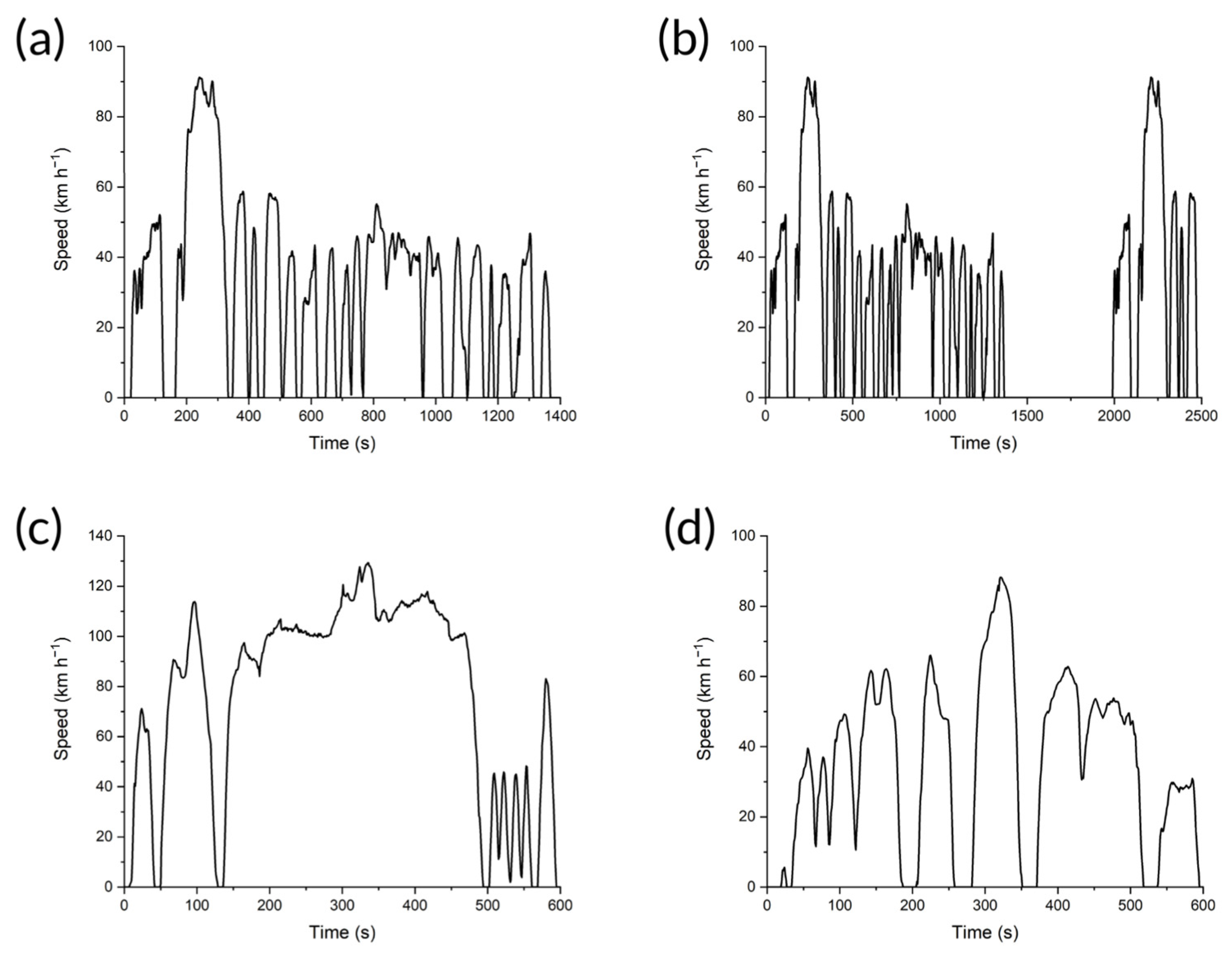
Figure 4.
Japanese legislative drive cycles. (a) The 10–15 Mode drive cycle was fully developed in 1991. It has a duration, average speed, and top speed of 660 s, 22.7 km h−1, and 70 km h−1, respectively. (b) The JC08 drive cycle was released in 2005. It has a duration, average speed, and top speed of 1204 s, 24.4 km h−1, and 81.6 km h−1, respectively.
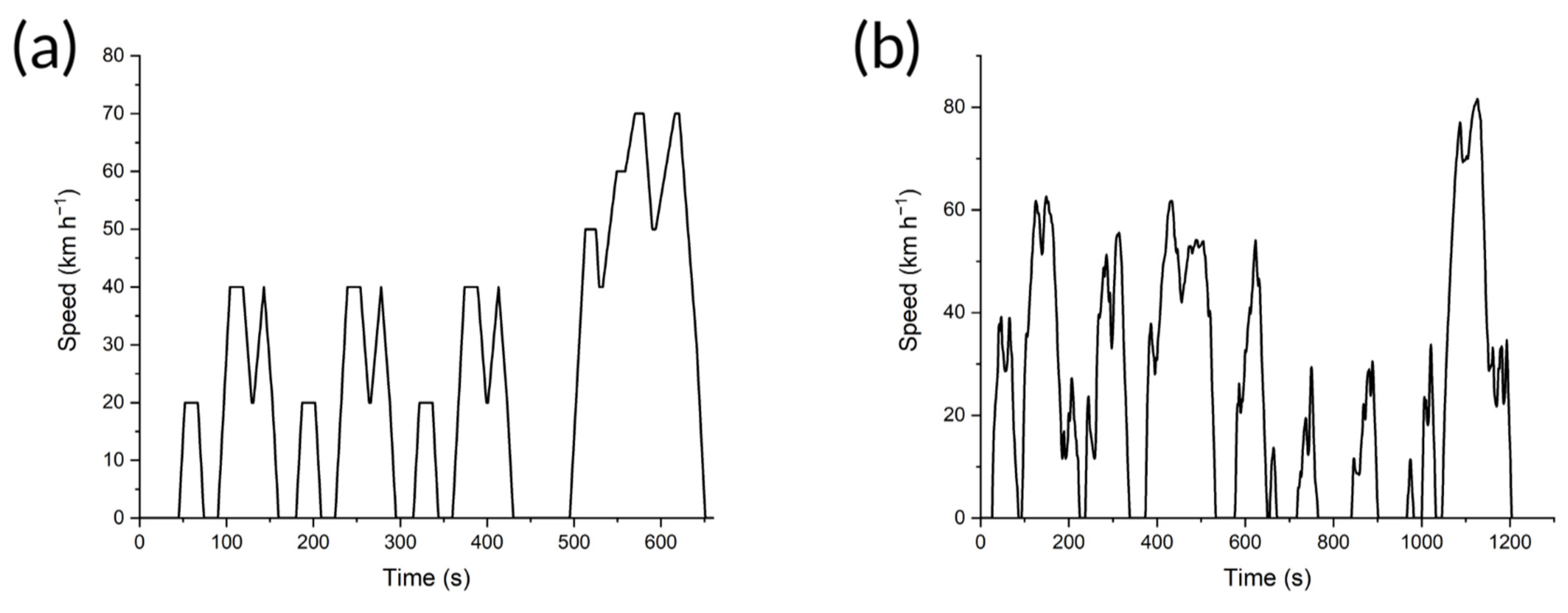

Figure 6.
Examples of aviation mission profiles. (a) Simplistic mission profile showing different stages and a reference elevation [48]. (b) Simplistic mission profile showing different stages and relative elevation changes [51]. The y-axis displays the altitude. (c) More detailed mission profile showing stages, groupings of stages, and altitude differences [52]. The y-axis displays the altitude.
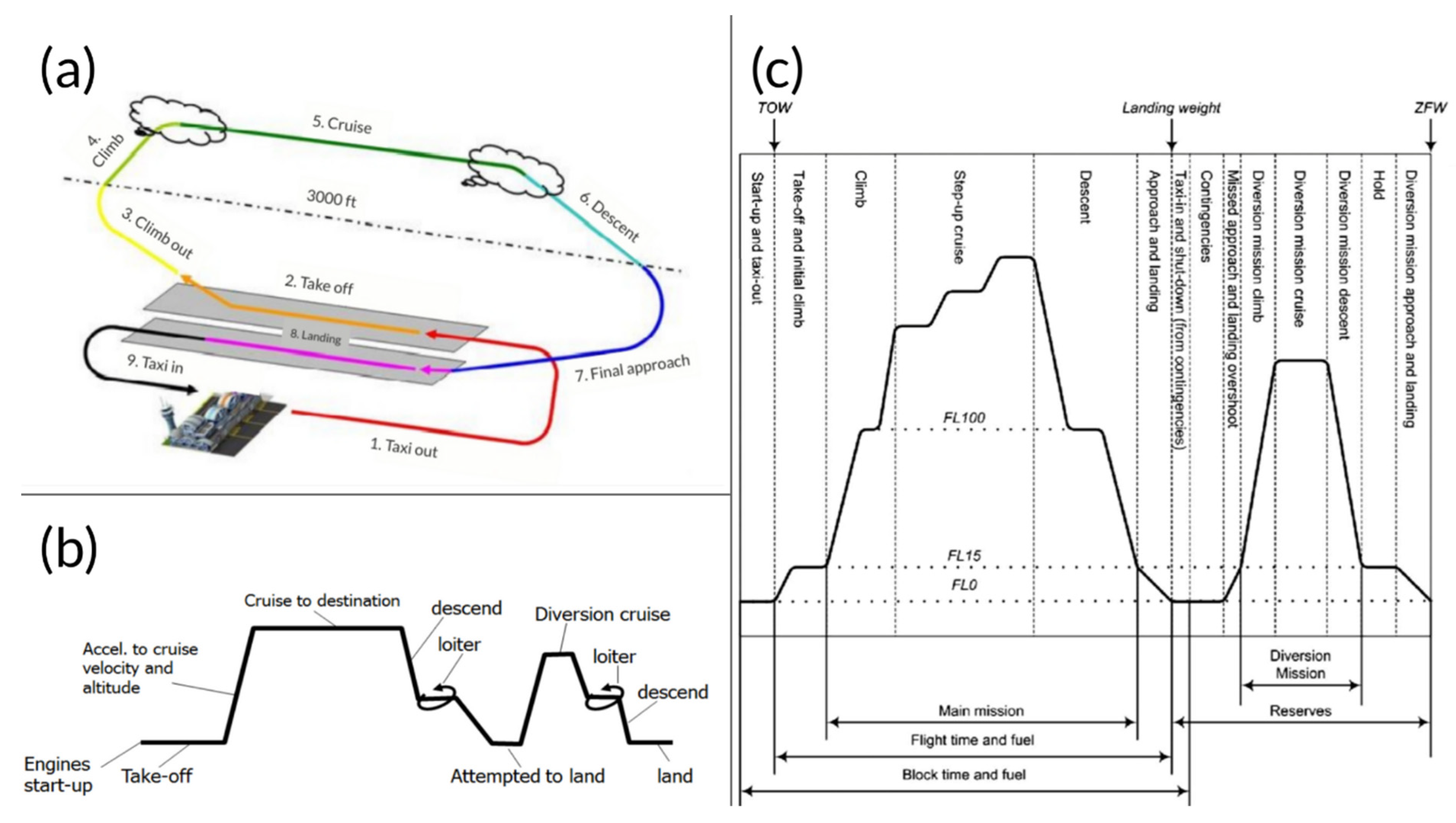
Figure 7.
Comparisons of legislative drive cycles. (a) Duration comparison. (b) Top and average speed comparisons. (c) Idle percentage comparison. (d) Acceleration and deceleration comparisons.
Figure 7.
Comparisons of legislative drive cycles. (a) Duration comparison. (b) Top and average speed comparisons. (c) Idle percentage comparison. (d) Acceleration and deceleration comparisons.

Figure 8.
Transient drive cycle development procedure using micro-trip clustering technique.
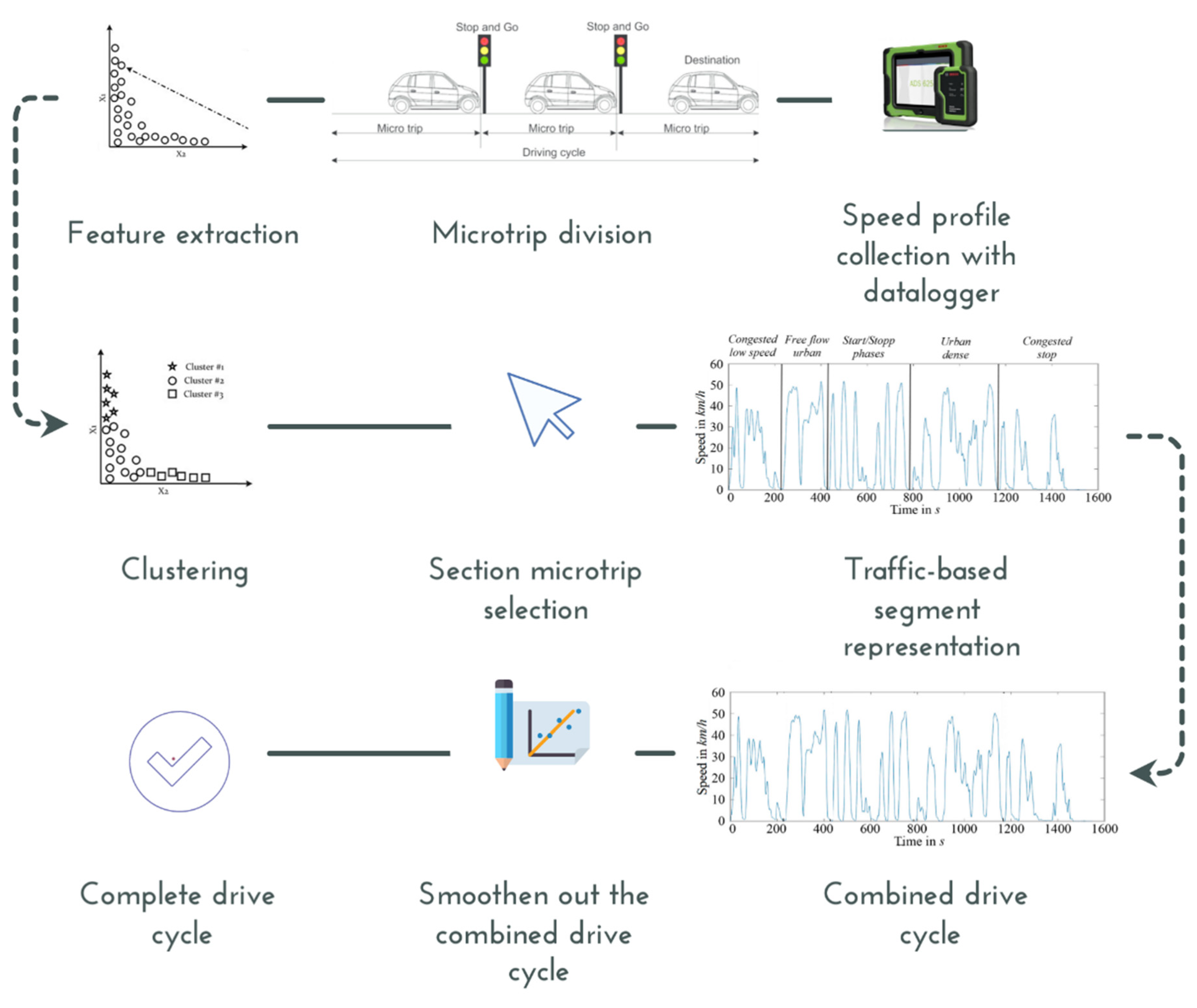
Figure 9.
Notation and schematics of the drive cycle to power cycle conversion. Fa, Fr, Fθ, and Fi are aerodynamic drag, rolling resistance, gradient resistance, and inertial force, respectively.
Figure 9.
Notation and schematics of the drive cycle to power cycle conversion. Fa, Fr, Fθ, and Fi are aerodynamic drag, rolling resistance, gradient resistance, and inertial force, respectively.

Figure 10.
Electrification level of battery-ICE vehicles [62,63]. This diagram can also be adapted for electrochemical hybrid vehicles.
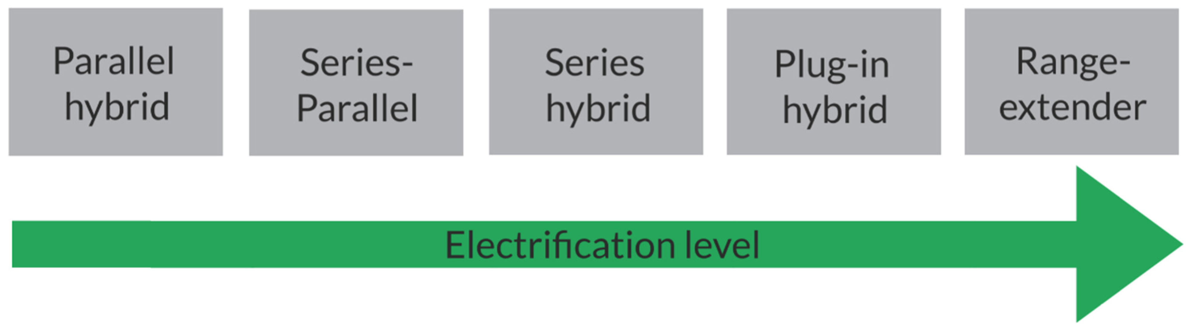
Figure 11.
Typical parallel architecture. This type of architecture allows propulsion by both the electric motors and ICE [60]. Some manufacturers may steer away from using power electronics to avoid power losses, creating what is known as a passive hybrid system [62].
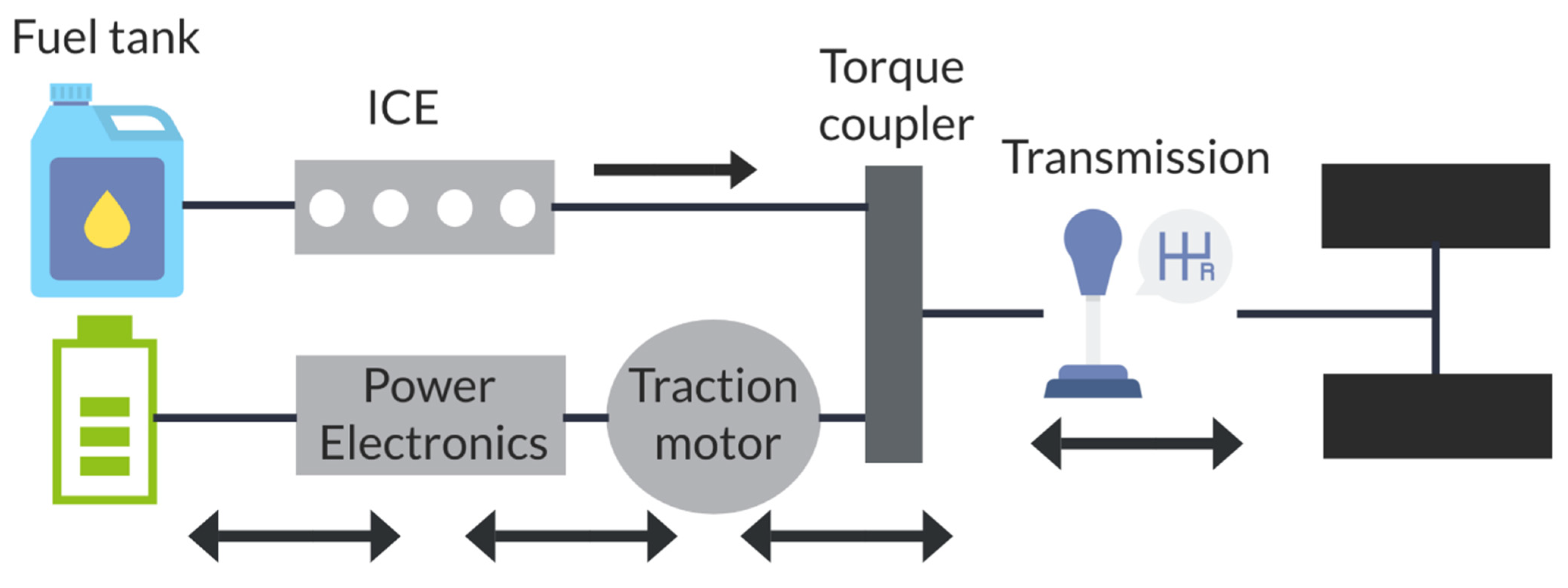
Figure 12.
Series and range-extender hybrid architecture. (a) Series architecture. In this architecture, only the electric motor paired with the battery is capable of propelling the wheels. The ICE is only used for charging. (b) Range extender. This architecture is similar to series architecture, except the ICE has less capacity, while the battery has more capacity.
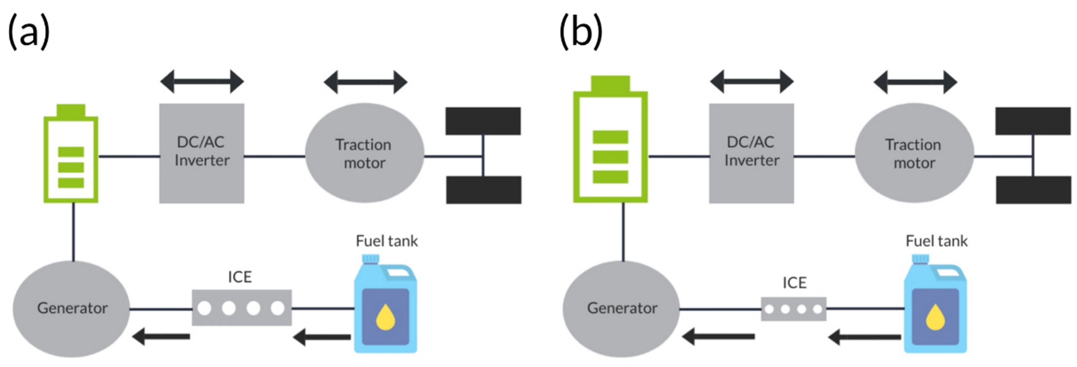
Figure 13.
Comparison of power and torque delivery characteristics of ICEVs and EVs. (a) Power and torque vs. engine speed graph for a typical ICEV [67]. (b) Power and torque vs. RPM graph for a typical EV or FCEV [67].
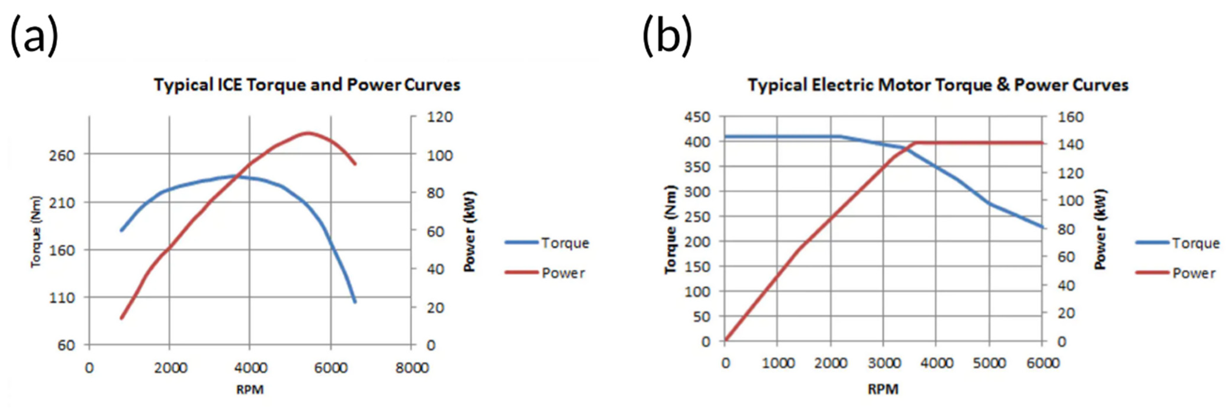
Figure 14.
Comparison between electric and CV motorcycle drive cycles in Khon Kaen City, Thailand (Koossalapeerom et al. [70]).
Figure 14.
Comparison between electric and CV motorcycle drive cycles in Khon Kaen City, Thailand (Koossalapeerom et al. [70]).
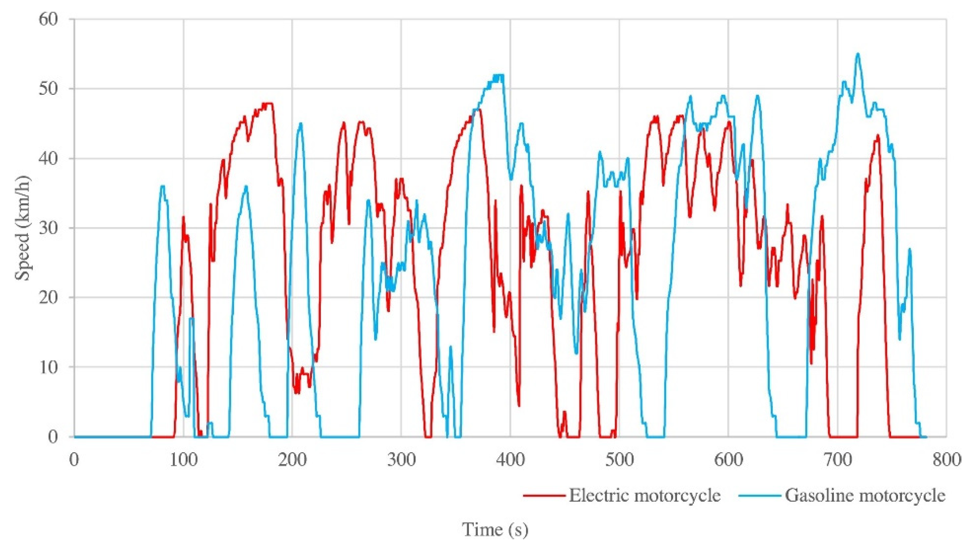
Figure 15.
Comparison of EV, hybrid, and CV LDV drive cycles during intermediate and harsh driving (Bogia et al.) [71].
Figure 15.
Comparison of EV, hybrid, and CV LDV drive cycles during intermediate and harsh driving (Bogia et al.) [71].
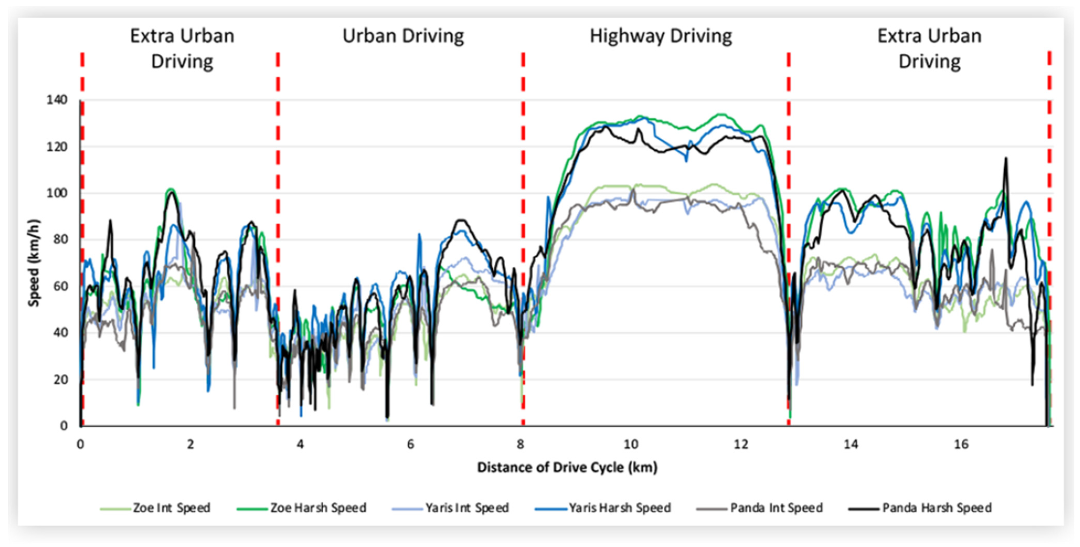

Table 1.
Mission profile list of stages and definitions [48].
Table 1.
Mission profile list of stages and definitions [48].
| Stage | Definition |
|---|---|
| Taxi-out | Travelling on land from parking area to runway |
| Take-off | Transition stage from land propulsion to air propulsion; aircraft takes off from the runway |
| Climb | Aircraft ascends to a predetermined cruising altitude |
| Cruise | Aircraft flying at optimal level to proceed to destination prior to descent, usually the longest stage |
| Descent | Aircraft decreases in altitude in preparation for landing |
| Final Approach | Aircraft positioned to start landing onto the runway |
| Landing | Aircraft returns to land propulsion mode |
| Taxi-in | Travelling on land from runway to parking area |
Table 2.
List of example drive cycle features and definitions [19].
Table 2.
List of example drive cycle features and definitions [19].
| Drive Cycle Feature | Definition |
|---|---|
| Average speed | Sum of all speed data values divided by the number of data points (equal to the total duration if datalogging interval is 1 s) |
| Idle time percentage | Ratio of time stopped divided by total time (percentage) |
| Velocity variance | Sum of the speed at a given time minus the average velocity squared, divided the total number of data points |
| Energy | Sum of squared speed values |
| Maximum speed | Maximum speed value |
| Minimum speed | Minimum speed value |
| Difference between maximum speed and minimum speed | Minimum speed subtracted from maximum speed |
| Average acceleration or deceleration | Sum of all acceleration or deceleration values divided by the total number of data points |
| Acceleration variance | Sum of the acceleration values at a given time minus the average acceleration, squared, divided by the total number of data points |
| Average acceleration | Sum of all acceleration values divided by the number of data points |
| Average deceleration | Sum of all deceleration values divided by the number of data points |
| Percentage of cruising | Time travelling at a constant speed divided total time (percentage) |
| Maximum acceleration or deceleration | Maximum value of acceleration or deceleration |
| Minimum acceleration or deceleration | Minimum value of acceleration or deceleration |
| Total distance | Total distance travelled (can be obtained by integrating the speed vs. time graph) |
| Average square acceleration | Sum of acceleration squared divided by the number of data points |
| Relative acceleration | Sum of speed values multiplied by acceleration at a given time over the total distance |
| Relative deceleration | Sum of speed values multiplied by deceleration at a given time over the total distance |
| Percentage of time when absolute acceleration and deceleration >1.5 m s−2 | Time during which the acceleration >1.5 m s−2 divided by the total time (percentage) |
| Percentage of time when absolute velocity times acceleration is between 3 and 6 m2 s−3 | Time during which the absolute velocity is between 3 and 6 m2 s−3 divided by the total time (percentage) |
Table 3.
Comparison of previous work on electric drive cycles and conventional drive cycles. Papers which use conventional CV drive to test electric vehicles are also included.
Table 3.
Comparison of previous work on electric drive cycles and conventional drive cycles. Papers which use conventional CV drive to test electric vehicles are also included.
| Author | Parameters Compared | Drive Cycles Used | Conclusions or Takeaway |
|---|---|---|---|
| Jeong et al. [15] | Performance evaluation, acceleration | Non-legislated Gwacheong, Korea drive cycle | Higher acceleration of electric motors not accurately represented in conventional drive cycles |
| Meddour et al. [68] | Battery sizing, electric motor cost, electric motor loss | WLTP, FTP-75, Artemis 150, and Artemis Urban | Torque demands vary drastically between drive cycles, choosing an accurate drive cycle is important |
| Zhao et al. [69] | Range estimation, energy consumption | XA-EV-UDC, FTP-72, FTP-75, JC08, 10–15 Mode, NEDC, and ECE-15 | Using conventional drive cycles for range estimation and energy consumption can produce a relative error as high as 38.14% and 21.17%, respectively |
| Koossalapeerom et al. [70] | Time spent during acceleration and deceleration, time spent cruising, speed, energy consumption, EV vs. CV | Non-legislated EV and CV motorcycle drive cycle in Khon Kaen City, Thailand | The EV drive cycle has less time spent during acceleration and deceleration, suggesting higher cruising times. Energy consumption of EV drive cycle can be as high as eight times lower than that of CV drive cycle |
| Borgia et al. [71] | Acceleration, deceleration, range estimation, intermediate vs. harsh driving, overall drive cycle attributes, EV vs. hybrid vs. CV | SEVCI, SEVCH, WLTP, NEDC | Acceleration and deceleration times are less for the EV when compared to CV, regenerative braking and electric motor characteristics are the main cause. |
Disclaimer/Publisher’s Note: The statements, opinions and data contained in all publications are solely those of the individual author(s) and contributor(s) and not of MDPI and/or the editor(s). MDPI and/or the editor(s) disclaim responsibility for any injury to people or property resulting from any ideas, methods, instructions or products referred to in the content. |
© 2023 by the authors. Licensee MDPI, Basel, Switzerland. This article is an open access article distributed under the terms and conditions of the Creative Commons Attribution (CC BY) license (https://creativecommons.org/licenses/by/4.0/).
Share and Cite
MDPI and ACS Style
Yang, J.D.; Millichamp, J.; Suter, T.; Shearing, P.R.; Brett, D.J.L.; Robinson, J.B. A Review of Drive Cycles for Electrochemical Propulsion. Energies 2023, 16, 6552. https://doi.org/10.3390/en16186552
AMA Style
Yang JD, Millichamp J, Suter T, Shearing PR, Brett DJL, Robinson JB. A Review of Drive Cycles for Electrochemical Propulsion. Energies. 2023; 16(18):6552. https://doi.org/10.3390/en16186552
Chicago/Turabian StyleYang, Jia Di, Jason Millichamp, Theo Suter, Paul R. Shearing, Dan J. L. Brett, and James B. Robinson. 2023. "A Review of Drive Cycles for Electrochemical Propulsion" Energies 16, no. 18: 6552. https://doi.org/10.3390/en16186552
Note that from the first issue of 2016, this journal uses article numbers instead of page numbers. See further details here.