Assessment of Driver Performance and Energy Efficiency in Transportation Tasks when Vehicle Weight Undergoes Significant Changes

Abstract

The results of the analysis of the operation of heavy-duty vehicles with high load capacity (tractor units with trailers) have been presented. The road transport of cargo relies heavily on vehicles of this type. Performing this role is associated with high energy consumption. Laden and unladen driving were investigated. The collected data guaranteed the constancy of numerous parameters, including the investigation of the same model vehicles under both loaded and unloaded conditions on identical roads. The assessment focused on changes in driving techniques and energy consumption during significant variations in vehicle weight. The evaluation was grounded in the measurement results of kinematic parameters, namely driving speed, acceleration, and braking deceleration. The aforementioned parameters are typically employed in analysing driving techniques (DBP—driver behaviour profile). The energy consumption of traffic was then assessed in light of the analysed changes in driving technique. The weight of the load was 24 t, increasing the weight of the vehicle by 175%. The increase in weight has caused a 68.4% increase in the energy required for driving. The change in vehicle mass has a relatively minor effect on the average, median, and modal values of driving speed. In contrast, the impact on acceleration is far greater. This is partly because the examined models of tractor units are equipped with high-power engines (420 hp). Furthermore, 81% of the roads used for transportation tasks are motorways and expressways.

1. Introduction

The domain of road freight transport represents an expanding sector where heavy-duty vehicles (HDVs) are an essential component of the overall system [1,2]. The HDV category of transportation is distinguished by its superior cost-effectiveness ratio, rendering it the most efficient mode in this regard. Within the territorial bounds of Poland, the HDV population exceeds 500,000 and exhibits a consistent growth pattern [3]. An essential feature of road freight transportation is its substantial fuel consumption. In tasks carried out using trucks, fuel expenditure constitutes between 30 and 41% of the total costs [4]. Conversely, within urban bus transportation [5], fuel expenditures cannot be as much as 75% of the total cost of ownership (TCO).

Heavy-duty trucks contribute to an estimated 25% of greenhouse gas emissions associated with road transport [6]. The operator significantly determines fuel consumption and emission levels, primarily by selecting driving techniques. Adjusting driving style represents a cost-effective and immediate strategy to drastically reduce fuel consumption and emissions [7,8]. Adopting fuel-efficient and eco-friendly driving practises in HDV operation has been identified as the most rapid approach to reducing emissions [9].

Over the past two decades, a growing body of research and publications has explored how the energy consumption of driving is dependent on the driving techniques used by drivers. The terms “driving technique” and “driving style” are commonly used in these publications, with the acronym DBP (driver behaviour profile) [10,11,12,13] also frequently employed. Within these works, authors typically focus on issues of ecology, with relatively little attention paid to the energy consumption of heavy-duty vehicle driving or the effects of significant changes in their weight.

Numerous studies on the topic of eco-driving are being published in parallel. The concept and its initial principles and research emerged in Scandinavian countries and Germany in the late 1990s. The European Union began supporting this initiative in 2001 by launching the Eco-Driving-Europe programme and continued with projects such as Ecodriven (2006–2008) and Ecowill (2010–2013) [14,15,16,17,18].

Many factors influence driving technique (driving style). The most important ones are the driver’s skills and experience, time of day, weather conditions, the type of road, and traffic organisation [19,20]. Similar findings result from [21]. There, it is stated that the load mass, average and standard deviation of speed, and driver’s driving style statistically correlate with fuel consumption by heavy-duty vehicles at a confidence level of 95%. With so many factors, identifying the impact of a single aspect on actual vehicle operation conditions is particularly difficult.

In a comprehensive review article [22], the authors delineate four primary determinants of vehicle energy consumption: the driver, vehicle and engine specifications, the organisation of roads and traffic, and prevailing weather conditions. Among these influential variables, elements tied to driving techniques warrant prioritisation due to the significant energy-saving potential associated with economical driving. Earlier studies underscore that economical driving can effectively achieve both fuel savings and emission reductions in the short term [22,23]. For vehicles equipped with internal combustion engines, the variation in fuel consumption attributed to different driving styles can reach between 15% and 25% [24]. In the case of hybrid vehicles (HV) and electric vehicles (EV), which can reduce deceleration, energy consumption is even more susceptible to the driving technique employed compared to their combustion-engine counterparts [25]. Research shows that for hybrid vehicles, the difference in fuel consumption due to divergent driving styles could drive economically; a reduction in energy consumption of up to 25% has been noted [25].

The literature on the influence of load mass on driving technique and energy consumption is limited. Previous studies have highlighted the need to investigate the effect of vehicle loading on driver behaviour [26]. As a result, an algorithm for evaluating driver performance was developed. While this issue is typically studied in the context of passenger vehicles, analysis of energy consumption in electric vehicles demonstrated that a 50% change in vehicle mass resulted in an average of a 25% change in energy consumption [27].

The authors have collated data on large trucks’ operational processes, specifically focusing on tractor units. Throughout the entirety of their usage period in the European Union (EU), a tractor unit, on average, covers a distance of 1,050,000 km [28]. Tractor units deployed in long-distance transport register an aggregate mileage of 1,470,000 km [15]. Estimates by the European Automobile Manufacturers’ Association (ACEA) suggest an annual mileage of 130,000 km within the EU [29]. Heavy-duty vehicles (HDVs) that have been in service for 8–9 years, on average, traverse between 110,000 and 135,000 km annually in the EU [28].

Throughout the data acquisition phase, a subset of routes was selected from an extensive collection of over 200 transport assignments within the investigated company. This selection was carried out to ensure the constancy of numerous parameters:

• In each course (transport task), the same driver operates the vehicle;
• Driving with and without a load takes place along essentially the same route (the same roads and streets). Differences arise from the presence of one-way roads, differently located access roads to expressways in the direction of the destination and return, or temporary road closures;
• The findings obtained from operating a single-vehicle model, specifically Scania R420 tractor units coupled with curtain-sided semi-trailers, were utilised in this study;
• Only courses with a uniform load weight of 24 t are analysed.

The dataset prepared for analysis included 20 transportation courses. Each of the courses comprised sections of driving on urban, suburban, motorway, and expressway roads. The need to take such road conditions into account during the assessment of driving energy consumption was indicated in [30,31]. It is considered that a single transport task consists of two parts, which have been named: loaded driving and unloaded driving. A separate analysis was conducted for the set of loaded drives and the set of unloaded drives, even though they are parts of the same transport task.

The aim of the research conducted is to assess the impact of significant changes in vehicle mass on driving technique and the resulting energy consumption of transport tasks. During this assessment, values and ranges of the variability of kinematic parameters describing the course of driving, as well as positional and modal statistics values, were analysed. Extreme courses with calm or dynamic characteristics were separately selected and classified. This classification also showed a correlation between mass change and energy consumption.

In truck testing, neither energy consumption nor emissions or exhaust composition are usually recorded directly. These characteristics are inferred indirectly by recording the kinematic parameters of the vehicle’s movement (speed and acceleration). As has been demonstrated in many previous works, these quantities are very strongly positively correlated with the general criteria mentioned above—energy intensity and exhaust emissions.

2. Methods

During data acquisition and preparation for further research, the following agreements and limitations were taken into account:

• The data collection process was based on a logistics company that organises and executes general cargo transport;
• The study was conducted between 2020 and 2022;
• One vehicle model was selected (tractor-trailer combination with curtain-sided semi-trailer, vehicle with combustion drive system, equipped with a tachograph with digital speed recording);
• The selected transport tasks are those in which it is possible to clearly distinguish between driving with and without a load. Driving without a load may involve returning from the unloading location to the transport base. Each of these drives should be at least 100 km long;
• Tasks were chosen for transportation that basically filled almost the entire workday of the driver or only slightly exceeded it (however, within the limits allowed by the law on drivers’ work time);
• The analysis focused solely on routes where cargoes of weight comparable to the maximum load-bearing capacity of the tractor-trailer unit were transported;
• Courses implemented in the lowland and flat areas were selected;
• Courses were selected so that each included driving on different types of roads (urban, suburban, expressways, and motorways).

The evaluation of the vehicle usage process and driving techniques employed by drivers was conducted through the measurement of physical quantities and the calculation of their corresponding statistical characteristics, specifically including:

• The speed of the vehicle;
• Acceleration during acceleration;
• The deceleration of a vehicle during the process of braking can result in a delay in the vehicle’s overall stopping time;
• The following characteristic values and statistics were considered:
• Arithmetic mean;
• Median as the middle value in the sample;
• Fashion as the most frequently occurring value in the sample;
• Standard deviation;
• Coefficient of variation, which is the quotient of the standard deviation and the arithmetic mean;
• Lower and upper quartiles, as the values below which 25% or above which 75% of the analysed sample’s values fall, are denoted in this paper by the symbols Q1 and Q3, respectively;
• Percentiles 10 and 90 are values below which 10% or 90% of the analysed sample falls, respectively. They are denoted throughout the study by the symbols P10 and P90;
• The skewness coefficient, indicated by the symbol As [32], is a statistical measure that quantifies the degree of asymmetry in a distribution. It is calculated by dividing the difference between the arithmetic mean and mode values by the standard deviation.

The value of population and occurrence indicators was reduced within a 100 km distance of the road.

The calculations performed enabled the determination of characteristic values for each individual ride and for the entire ensemble of rides under examination. The inferential process was executed in multiple phases. Initially, the values of the aforementioned variables were ascertained. Subsequently, outlier journeys were identified. The analyses of loaded and unladen journeys were conducted independently.

In order to determine the energy consumption of motion, the total energy required to overcome resistance during HDV driving at a specific speed and the kinetic energy during acceleration phases were calculated. Additionally, an analysis of driving techniques was conducted with a focus on eco-driving principles, such as:

• limiting intense acceleration;
• Avoiding sudden braking;
• Maximum speed limit;
• Aim to maintain a constant driving speed for the longest possible stretches.

3. Results of Research and Statistical Analysis of Vehicle Kinematics during Loaded and Unloaded Driving

3.1. Analysis of Driving Speed

The speed of driving during the implementation of a transport task depends, among other things, on legal restrictions, traffic intensity, the traction properties of the vehicle, and the driver’s actions. High efficiency in vehicle utilisation is achieved by transport companies at high driving speeds.

The study involved a two-part analysis of driving speeds. In the first part, characteristic values and statistics were obtained for individual trips, and two trips with extreme values were identified. The calculations were performed separately for loaded and unloaded trips. In the second part, the statistical characteristics of loaded and unloaded trips were compared.

The diagram in Figure 1 depicts an illustration of the speed profile for an individual journey, specifically referring to a transportation task or route.

Figure 2 provides a summary of the average speed values of all the courses analysed. The numbering of courses follows the order in which they are qualified for the dataset.

3.1.1. Load Speed Analysis

Table 1. Examples of characteristic values and statistics calculated from the laden speed course.

Course Designation	Course Length	Avg. Speed	Median	Mode	Maximum	K25	K75	P10	P90	Std. Deviation	Coefficient of Variation
Median	km	m/s	m/s	m/s	m/s	m/s	m/s	m/s	m/s	m/s	---
1	297	22.3	24.1	24.7	27.2	21.6	24.7	17.7	24.8	4.4	19.9
2	176	21.5	23.1	24.6	26.6	21.1	24.3	15.0	24.7	4.7	21.9
3	175	14.5	16.1	16.6	25.1	11.7	18.4	5.6	20.2	5.5	38.0
4	194	19.9	23.1	24.7	26.4	18.6	24.4	7.9	24.6	6.7	33.6
5	161	19.3	23.3	24.8	26.1	14.7	24.7	8.8	24.7	6.8	35.3

shows selected values and statistics that were calculated based on the speed of the loaded vehicle.

Utilising the characteristic values and statistics for the set of courses under analysis (illustrated in Table 1), two outlier drives were identified and labelled: calm driving (NS) and dynamic driving (DY). The nomenclature for these outlier drives was partially influenced by literature wherein a scale was employed to rate driver behaviour, with descriptors ranging from aggressive to normal to calm (cautious) [26,33,34]. The selection of drives was facilitated using a ranking methodology.

Characteristic values of speed, both for individual courses (e.g., Table 1) and for averages from 20 courses (Figure 2) deviate significantly from a normal distribution. One can use the expression that there are many outliers in each case (this also applies to acceleration during acceleration and deceleration delays analysed later in this paper). These properties make the rank method the most favourable method for further analysis and evaluation of the characteristic values for a set of courses. Rank methods, in contrast to parametric methods [35]:

• They do not require any assumptions about the distribution of the population;
• They are resistant to outlier observations;
• They can process variables on an ordinal scale.

The process of ranking involves ordering observations based on a single variable and assigning them new values in the form of ranks. The rank is determined by the consecutive numbering of observations after sorting them according to the variable value. This method is particularly useful in cases where outliers are present, as it eliminates information about the difference between consecutive observations. Multiple-criteria ranking, which utilises more than one feature criterion, was employed to establish the final results based on the total ranks.

Two of the widely recognised eco-driving principles relating to vehicle speed were applied: limiting maximum speed and striving to maintain a steady speed for longer durations (minimising reductions in speed). Among the statistics presented in Table 1, the mean value and standard deviation were considered the most credible for these criteria. In order to further reinforce the criterion of minimising speed fluctuations, a third statistic, the coefficient of variation, was appended to these two. Three rankings were established: mean value, standard deviation, and coefficient of variation. The overall rank was computed as the sum of the ranks of the three statistics for each course. Each individual ranking was given a value of 1.

The extreme rides selected in this way are:

• smooth running, NS, course 3;
• dynamic driving, DY, course no. 12.

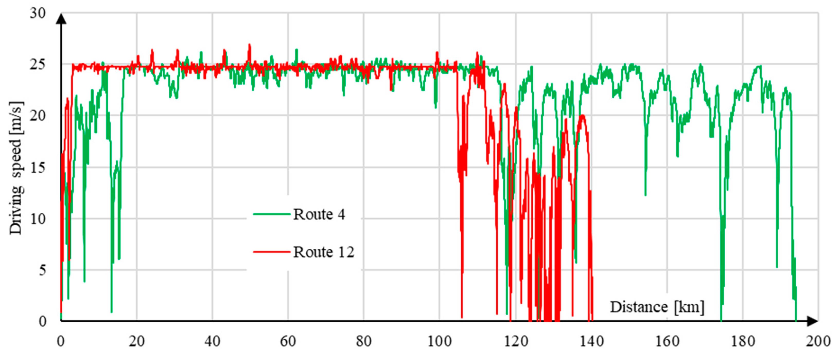
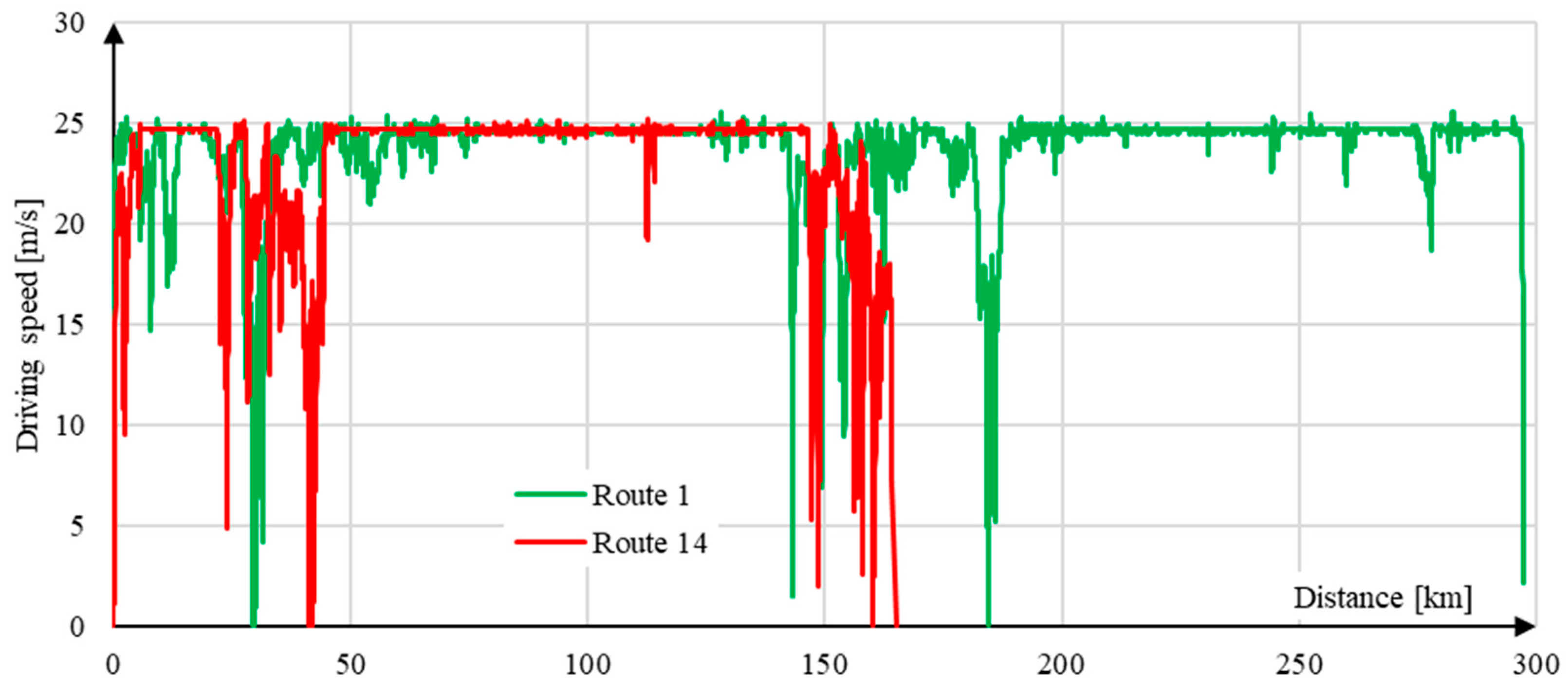
The chart in Figure 3 illustrates the speed profile with respect to distance for the selected courses, exhibiting high variability of speed and complex changes in its characteristics. Two profiles exhibit distinct differences in their behaviour during the journey. Evaluating the dynamics of these changes can be achieved by analysing the characteristic values obtained from

Table 2. Characteristic values from the speed waveform for extremely laden journeys and average values for the entire set of laden journeys.

Name	Course Designations	Average	Median	Mode	Std. Deviation	P10	K25	K75	P90
Median		m/s	m/s	m/s	m/s	m/s	m/s	m/s	m/s
Calm driving (NS)	3	14.6	16.1	16.7	5.5	5.6	11.7	18.4	20.3
Dynamic driving (DY)	12	18.1	24.0	24.7	8.5	3.3	11.4	24.7	24.8
Average values for 20 laden journeys (M)	--	19.3	21.9	24.2	6.3	9.0	16.9	23.8	24.4

. Though the selected courses have only a few features of calm and dynamic driving, referring to the values from the entire set of courses (Table 2) can assist in inferring significant differences in driver behaviour in loaded and unloaded conditions.

Figure 3 and Table 2 illustrate, among other elements, the similarities and differences in the driver’s engagement with the vehicle and their responses to prevailing traffic conditions. This is effectively depicted through a comparison with the mean values for the entire dataset (courses).

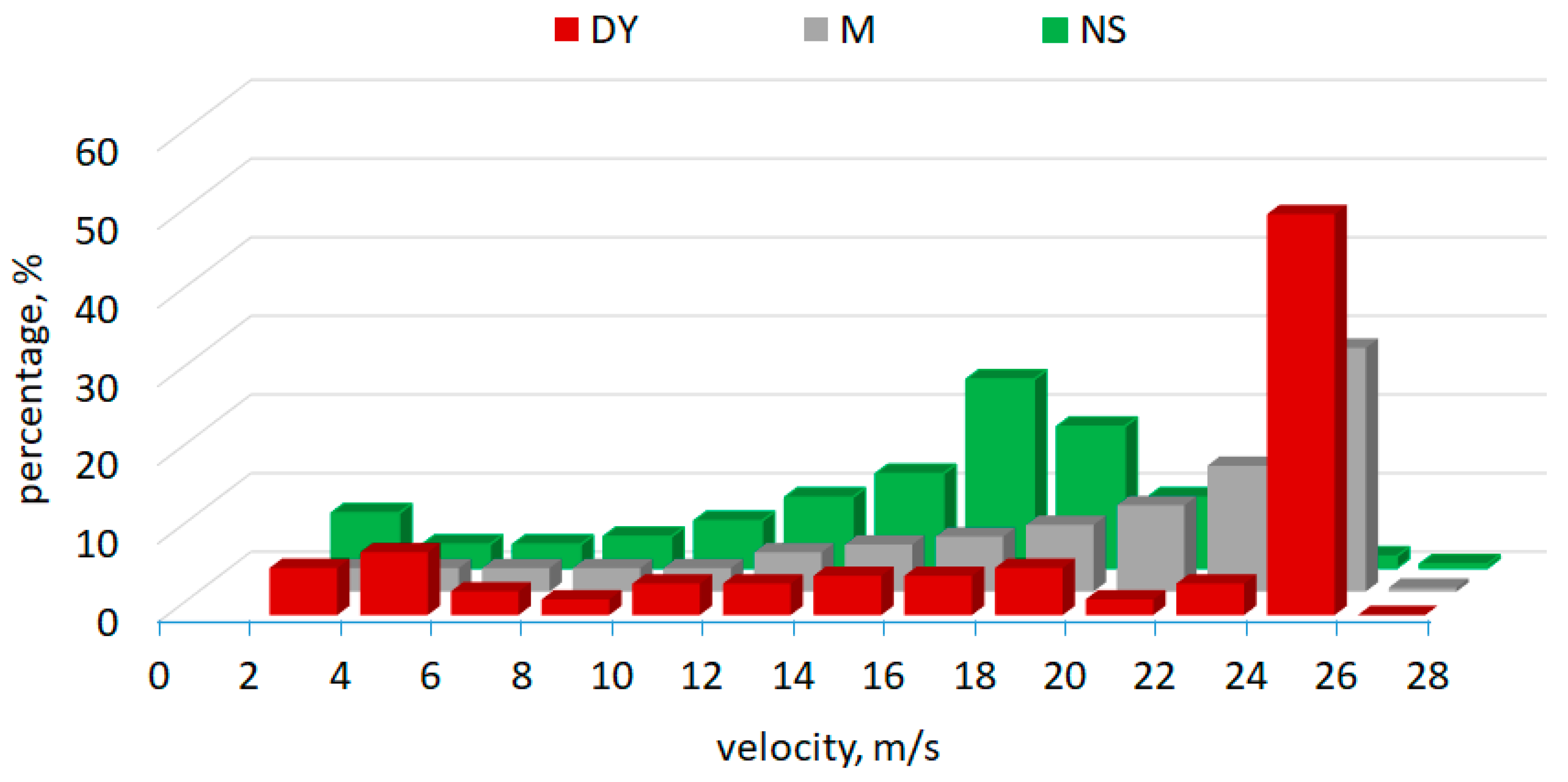
Figure 4 delineates the percentage distribution of travel speed occurrences within prescribed speed intervals. The percentage distribution quantifies the proportion of travel speed instances within individual speed intervals relative to the total for the entire loaded journey segment. This enables a comparison of the results obtained from courses of varying lengths. The employed travel speed intervals possess a width of 2 m/s. These values are contrasted with the averages, which are computed for the entire collection of laden journeys. Within the figure, the values are presented in the sequence of drives: dynamic (DY), averaged (M), and calm (NS).

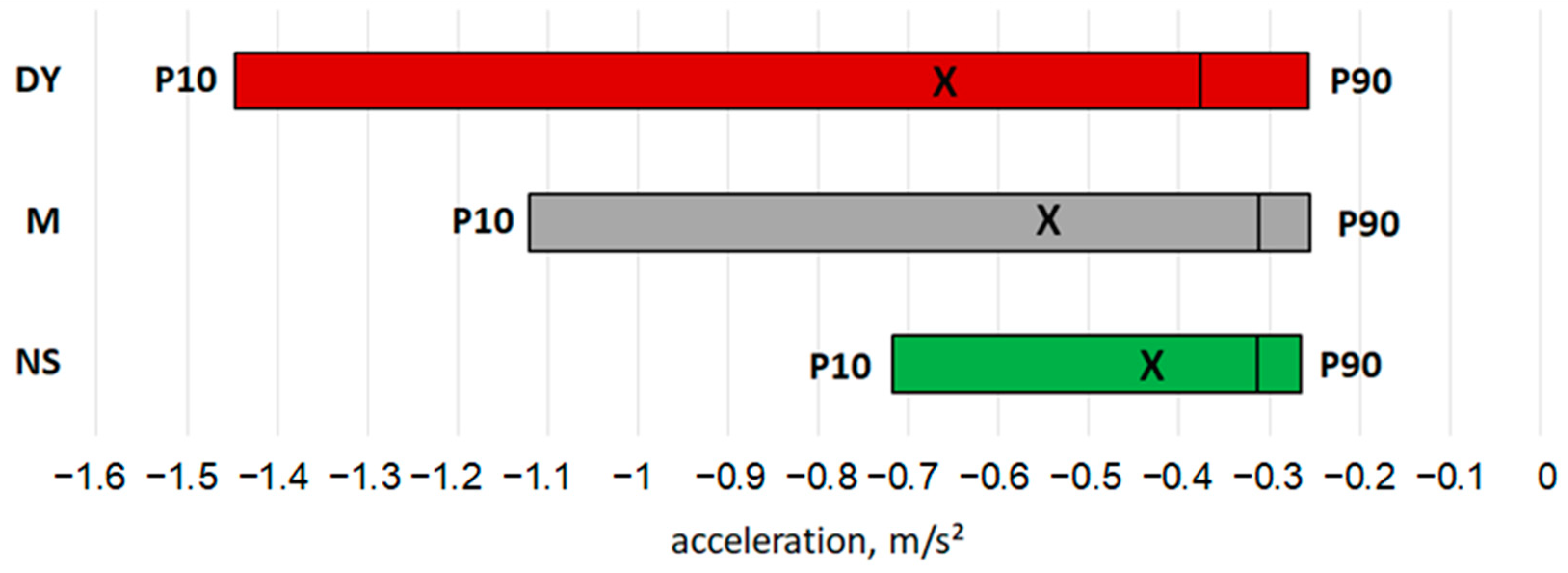
Due to the very specific forms of the distributions shown in Figure 4, the values of mean, median, P10, and P90 are additionally summarised in Figure 5 (the numerical values of these statistics are given in Table 2).

Figure 5 illustrates that the driving style labelled “most dynamic” (DY) exhibits the greatest range of driver speeds achieved, as evidenced by the length of the interval between the 10th and 90th percentiles (P10 and P90). Furthermore, a noteworthy characteristic of this driving style is the proximity of the median and P90 values, as well as the modal value (refer to Figure 4 and Figure 5 and Table 2). It is also notable that for the mean of 20 drives (M), the modal value and P90 exhibit values in close proximity to one another.

Separately, the energy intensity of driving (related to 1 km of distance travelled) was calculated for both extreme drives, which is:

• Smooth driving, course 3, 1565 MJ/175 km = 8.94 MJ/km
• Dynamic driving, course 12, 1391 MJ/140 km = 9.91 MJ/km.

This means that the energy intensity of DY driving was 8.7% higher than that of NS driving.

3.1.2. Analysis of Unladen Speed

The analysis was carried out in a similar way to that for laden driving.

Table 3. Exemplary characteristic values of speed during unloaded driving.

Course Designation	Course Length	Avg. Speed	Median	Mode	Maximum	K25	K75	P10	P90	Std. Deviation.	Coefficient of Variation
Median	km	m/s	m/s	m/s	m/s	m/s	m/s	m/s	m/s	m/s	---
1	297	22.9	24.7	24.7	25.6	23.6	24.5	18.7	24.4	4.3	18.9
2	171	22.5	24.4	24.6	25.3	22.5	24.7	17.6	24.7	4.3	19.0
3	177	15.1	16.7	18.1	25.8	12.9	18.5	7.5	20.2	5.1	33.5
4	195	20.7	23.6	24.6	25.4	18.8	24.2	12.2	24.6	5.6	27.1
5	162	20.3	23.5	24.8	25.0	17.5	24.6	11.2	24.8	6.0	29.5

shows examples of characteristic values and speed statistics for unladen driving.

The statistical values obtained from all unloaded rides (as shown in Table 3) were utilised for the selection of extreme rides. The ranking process was the same as that used for the analysis of loaded rides. The outcome of the selection of calm and dynamic rides is presented below:

• smooth running, NS, course 3;
• dynamic driving, DY, course no. 11.

It should be emphasised that the same route (with the same driver) was chosen for calm driving as for driving with a load. However, for dynamic driving, the ranking result indicated a different route than before.

Figure 6 displays velocity profiles during driving, while

Table 4. Characteristic values calculated from the speed waveform for selected unladen journeys.

Name	Course Designations	Average	Median	Mode	Std. Deviation	P10	K25	K75	P90
Median		m/s	m/s	m/s	m/s	m/s	m/s	m/s	m/s
Calm driving (NS)	3	15.1	16.8	18.1	5.1	12.9	18.4	7.5	20.2
Dynamic driving (DY)	11	20.9	24.6	24.7	6.2	19.5	24.7	11.1	24.7
Average values for 20 laden journeys (M)	--	20.3	22.7	24.3	5.5	18.6	24.0	12.1	24.4

presents several characteristic quantities for selected drives. Similar to the previous section, to ease the evaluation of the dynamic changes in speed for both selected extreme drives, the values that characterise them have been collated in the table with statistics calculated for the entire set of drives (20 drives in total).

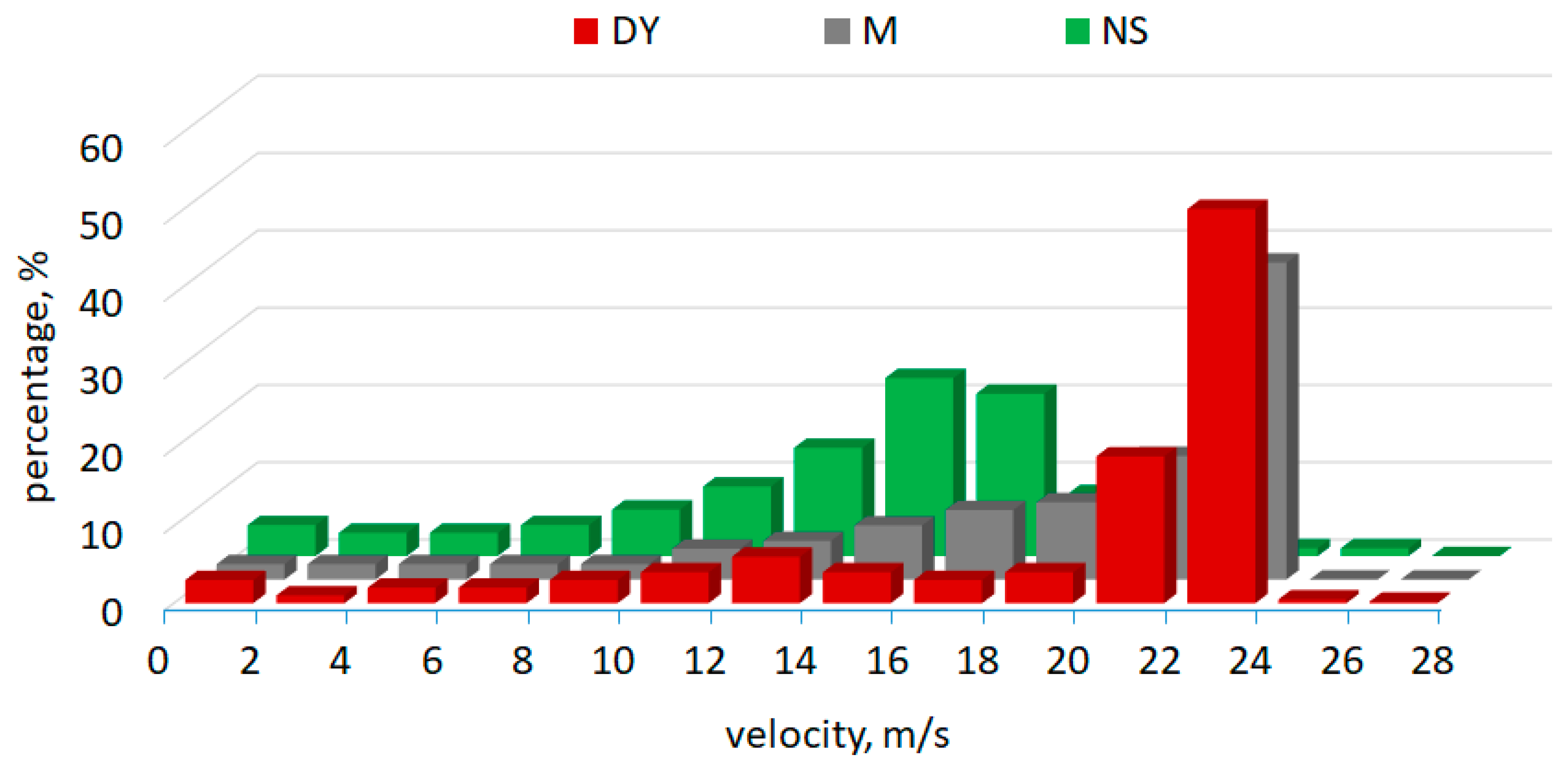
In Figure 7, histograms of the percentage distribution of the number of values of speed without cargo are shown. A percentage approach is used to compare courses of different lengths. The values in each speed range are compared to the mean values calculated for the entire set of drives without cargo.

As in the previous case, due to the very specific forms of the distributions shown in Figure 7, the values of mean, median, P10, and P90 are additionally summarised in Figure 8 (the numerical values of these statistics are given in Table 4).

Contrary to loaded driving, during unloaded driving, the spectrum of speeds attained by the driver (the interval length between P10 and P90) does not demonstrate substantial deviation from either NS driving or the mean of 20 drives (M). Nevertheless, the second characteristic previously identified as significant for unloaded driving, namely the congruence of median and P90 values as well as the modal value (refer to Figure 8 and Table 4), remained consistent. In the present scenario, these values are even more closely aligned than during loaded driving. Similarly, in this context, the modal value and P90 (calculated as the mean of 20 drives) exhibit remarkably close values.

Energy consumption during the aforementioned unloaded drives (per 1 km of distance travelled) was also calculated. The specific energy consumption is:

• Smooth driving, course 3, 803 MJ/177 km = 4.54 MJ/km;
• Dynamic driving, course No. 11, 508 MJ/88 km = 5.77 MJ/km.

This indicates that the energy efficiency of DY driving was notably lower than that of NS driving, with a significant difference of 27.1% in energy consumption. This disparity is evident not only in percentage but also in absolute terms, with a 0.78 MJ/km and 1.23 MJ/km difference for loaded and unloaded driving, respectively.

3.2. Analysis of Acceleration during Speeding Up

The acceleration process during speeding up is dependent on several factors, including the capabilities of the vehicle’s driving system, the driver’s actions, and the road situation. The driver’s actions are particularly important and involve selecting:

• gear ratios in the gearbox;
• the rate and extent of pressure on the accelerator pedal.

The semi-trailer tractor model analysed can achieve the accelerations shown in

Table 5. Acceleration values achievable by the vehicle under consideration [36].

Running Number	Running Speed, m/s	Acceleration Achieved, m/s2
1–2 gear	0–3	0.7–0.94 loaded 2.49–2.62 unladen
6–8 gear	10–15	0.2–0.4 loaded 0.82–1.24 unladen

.

Figure 9 summarises the average acceleration values of all the courses analysed.

3.2.1. Acceleration of the Vehicle (a > 0) When Driving Loaded

In

Table 6. Examples of characteristic values determined from positive acceleration values (a > 0).

Course Designation	Path during Acceleration	Avg. Speed	Median	Mode	Maximum	K25	K75	P10	P90	Std. Deviation.	Coefficient of Variation
Median	km	m/s	m/s	m/s	m/s	m/s	m/s	m/s	m/s	m/s	---
1	13	0.326	0.278	0.230	0.940	0.232	0.390	0.230	0.556	0.153	46.8
2	7	0.334	0.289	0.232	0.938	0.230	0.391	0.233	0.544	0.133	40.0
3	23	0.398	0.324	0.266	0.940	0.266	0.440	0.231	0.683	0.187	47.1
4	10	0.333	0.289	0.230	0.833	0.231	0.394	0.228	0.532	0.122	36.5
5	9	0.382	0.371	0.278	0.938	0.277	0.440	0.231	0.590	0.148	38.7

, physical quantities have been compiled, similar to the analysis of driving speeds. These are examples of courses from a set of 20 rides. The length of the road in the second column is the distance travelled by the vehicle during the acceleration phase.

The selection of two extreme rides with a load was made based on the statistical values calculated from the acceleration data in the analysed set of courses (examples are provided in Table 6). Characteristic values of acceleration, both for individual courses (e.g., Table 6) and for averages from 20 courses (Figure 9) diverge significantly from the normal distribution. Thus, in this case, the rank method is the most suitable approach for subsequent analysis and assessment.

During the selection process, the fact that the top criterion for eco-driving, as identified among the four most frequently repeated criteria, is limiting intensive acceleration, was utilised. A further frequently mentioned criterion was identified as the “economical” operation of the acceleration pedal. The mean value was considered the most reliable statistic for the first criterion, whereas the standard deviation was chosen for the second. To further enhance the criterion of minimising frequent acceleration changes, a third statistic, the coefficient of variation, was added to the analysis, similar to the approach taken with speed analysis.

For the set of courses analysed, three rankings were prepared. The overall rank was determined as the sum of the ranks of three statistics for each course.

Selected extreme driving styles (due to acceleration) include:

• calm driving, NS, course 4;
• dynamic driving, DY, course 12.

It is important to note that the same route (with the same driver) was selected for dynamic driving as it was used for speed analysis with a load. In terms of calm driving, the ranking result showed a different route than previously.

Figure 10 presents speed profiles for the aforementioned courses. These profiles show the frequency and dynamics of the vehicle acceleration process with a load. To facilitate the analysis of the driver’s behaviour during these courses,

Table 7. Characteristic values from the acceleration curve for the laden journeys analysed.

Name	Course Designations	Average	Median	Mode	Std. Deviation	P10	K25	K75	P90
Median		m/s2	m/s2	m/s2	m/s2	m/s2	m/s2	m/s2	m/s2
Calm driving (NS)	4	0.333	0.289	0.230	0.122	0.231	0.394	0.228	0.532
Dynamic driving (DY)	12	0.398	0.359	0.232	0.176	0.266	0.509	0.231	0.660
Average values for 20 laden journeys (M)	---	0.354	0.300	0.230	0.147	0.247	0.416	0.230	0.570

lists characteristic values for selected extreme drives. These values are also compared to statistics calculated for the entire set of drives with a load.

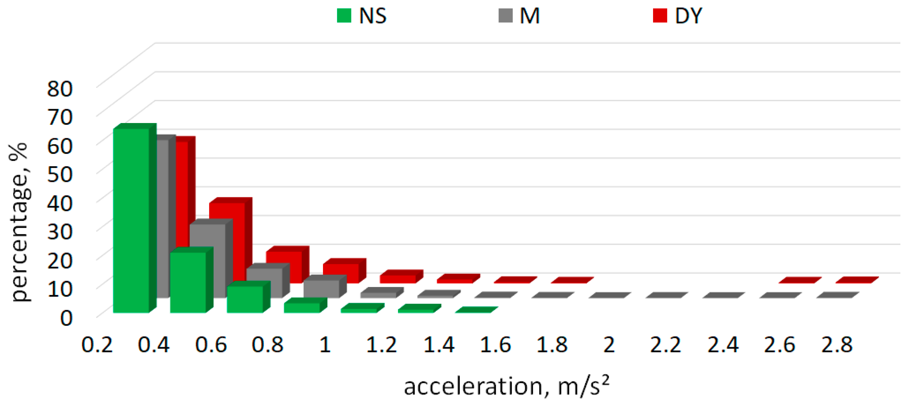
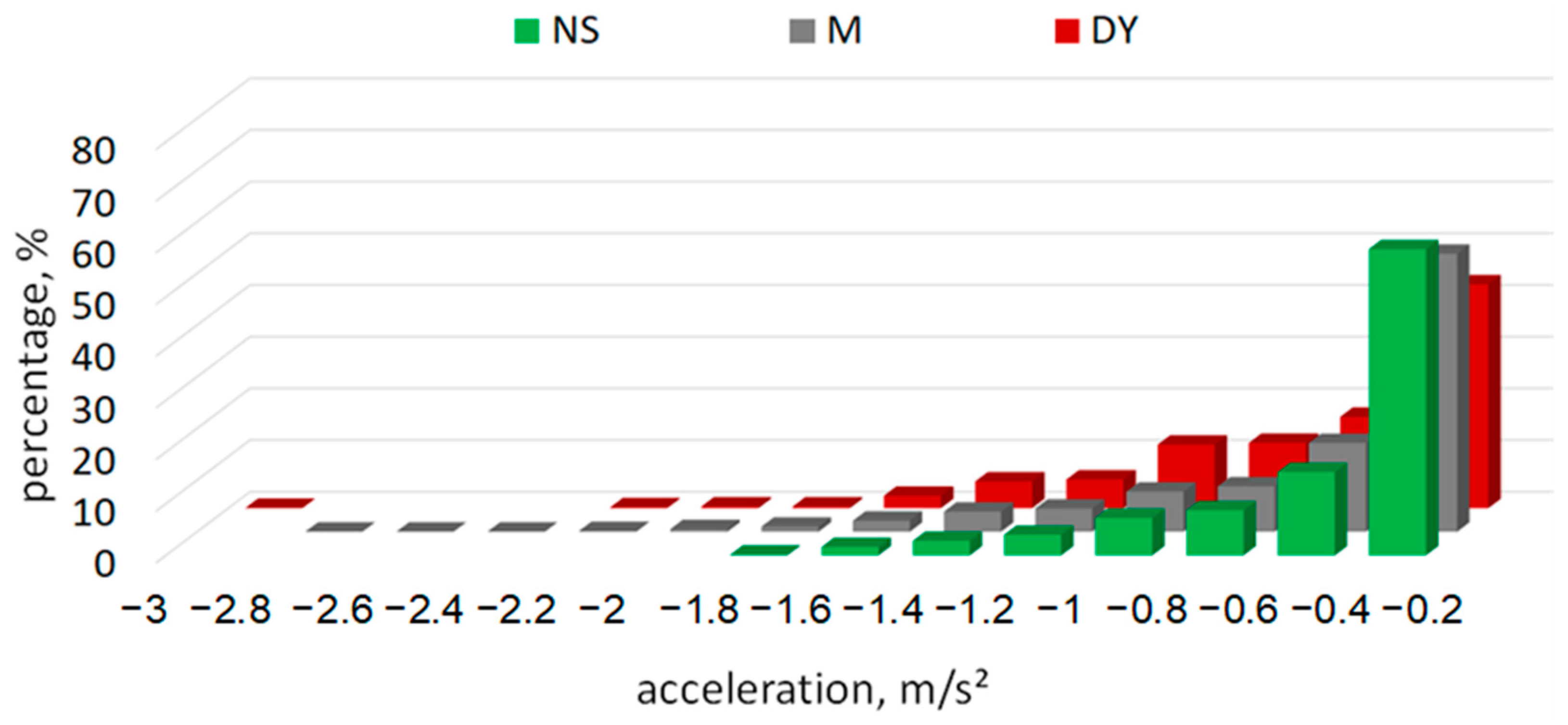
The percentage distribution of acceleration values during acceleration (a > 0) in the analysed courses is displayed in Figure 11. The acceleration values occurring during extreme courses are compared to the mean values (M), which are calculated for all rides with a load.

Due to the very specific forms of the distributions shown in Figure 11, the values of mean, median, P10, and P90 are additionally summarised in Figure 12 (the numerical values of these statistics are given in Table 7).

The initial observation of note is that P10 values for all three cases (NS and DY driving, in addition to the overall set of drives—M) exhibit a near-equivalent value of 0.23 m/s², as evinced in Table 7. The modal value atop of this is also the same for these cases (Table 7) and is equal to P10. This denotes the acceleration obtained from the 8–10 gears during acceleration while driving with a load. Figure 12 further demonstrates that the drive designated as the most dynamic is characterised by the widest spectrum of accelerations accomplished by the driver, as denoted by the length of the interval between P10 and P90. A commensurate situation was also noted during the examination of speeds for drives with a load.

Separately, the energy intensity of driving was calculated, which is related to 1 km travelled:

• Smooth running, course 4, 1864 MJ/194 km = 9.61 MJ/km;
• Dynamic driving, course 12, 1391 MJ/140 km = 9.91 MJ/km.

This means that the energy intensity of DY driving was, in this case, only 3.1% higher than that of NS driving.

3.2.2. Acceleration of the Vehicle (a > 0) When Driving Unladen

The characteristic values obtained from the acceleration profiles of five unloaded vehicle drives are exemplified in

Table 8. Summary of characteristic acceleration values (a > 0) when driving unladen.

Course Designation	Path during Acceleration	Avg. Speed	Median	Mode	Maximum	K25	K75	P10	P90	Std. Deviation.	Coefficient of Variation
Median	km	m/s2	m/s2	m/s2	m/s2	m/s2	m/s2	m/s2	m/s2	m/s2	---
1	12	0.406	0.278	0.276	1.528	0.277	0.440	0.260	0.694	0.209	51.4
2	6	0.425	0.290	0.265	2.620	0.266	0.509	0.266	0.764	0.247	58.2
3	23	0.416	0.312	0.266	2.361	0.267	0.498	0.267	0.717	0.214	51.4
4	14	0.433	0.382	0.279	1.447	0.278	0.544	0.265	0.729	0.212	49.1
5	11	0.459	0.393	0.266	1.748	0.279	0.567	0.266	0.798	0.230	50.2

. The distance travelled by the vehicle during the acceleration phase is indicated in the second column.

Based on the characteristic values derived from the acceleration profile during the acceleration of an unloaded vehicle (examples are provided in Table 8), outlier driving modes were selected. It is postulated that the driver might not need to employ identical driving strategies when accelerating a loaded or unloaded vehicle. The ranking procedure paralleled the one used in the analysis of load driving. The outcome of choosing calm and dynamic driving modes is as follows:

• Smooth running, NS, course 1;
• Dynamic driving, DY, course no. 12.

It is important to note that the same route (with the same driver) was utilised for dynamic driving as was employed for the analysis of velocity and acceleration during driving while carrying a load. For peaceful driving, the ranking outcome identified an alternative route to that of the preceding instances.

Figure 13 shows the travel speed waveform for the above-selected courses.

The speed profiles were utilised to compute various acceleration statistics and characteristic values during the acceleration phase for runs 1 and 12. These values were then compared to the average values obtained from the complete set of unloaded runs. The results are tabulated in

Table 9. Characteristic values calculated from the acceleration curve for unladen journeys.

Name	Course Designations	Average	Median	Mode	Std. Deviation	P10	K25	K75	P90
Median		m/s2	m/s2	m/s2	m/s2	m/s2	m/s2	m/s2	m/s2
Calm driving (NS)	1	0.406	0.278	0.276	0.209	0.277	0.440	0.260	0.694
Dynamic driving (DY)	12	0.484	0.405	0.278	0.291	0.278	0.567	0.255	0.845
Average values for 20 laden journeys (M)	---	0.447	0.371	0.272	0.242	0.277	0.543	0.2638	0.770

.

The diagram presented in Figure 14 illustrates the distribution of acceleration values observed during unloaded rides. This distribution represents the percentage occurrence of acceleration values for courses 1 and 12. The percentage acceleration share values are then compared to the mean values for the entire set of unloaded courses.

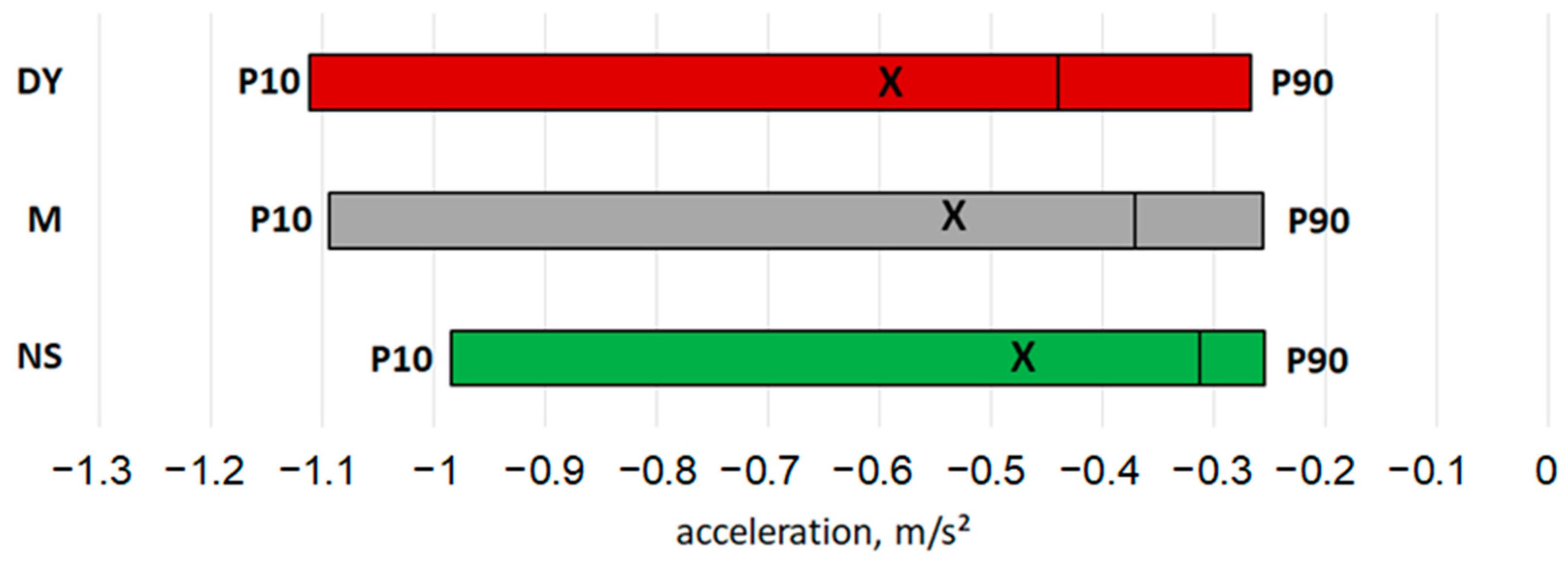
In a comparable manner to the previous analysis, in order to showcase unique features of the acceleration value distribution, Figure 15 presents the values of the mean, median, P10, and P90. The numerical data for these statistics can be found in Table 9.

Figure 15 illustrates (in a manner analogous to that earlier presented for laden driving in Figure 12) that the most dynamic unladen driving is distinguished by the widest range of accelerations executed by the driver (the longest interval between P10 and P90). A second noteworthy feature of this driving mode is that, despite instances of accelerations slightly surpassing 2.6 m/s² being recorded (Figure 14), drivers predominantly accelerate the vehicle with accelerations considerably lower than the maximum achievable. This is substantiated by the P90 values presented in Figure 15 and, in the case of NS driving, additionally by the absence of recorded accelerations exceeding the 1.6 m/s² value in Figure 14.

The energy consumption of driving without load for the analysed extreme rides has been calculated and found to be:

• Smooth running, course 1, 1791 MJ/297 km = 5.53 MJ/km;
• Dynamic driving, course 12, 848 MJ/145 km = 5.85 MJ/km.

This means that the energy intensity of DY driving was 5.8% higher than that of NS driving.

3.3. Activity Analysis of the Braking Process (a < 0)

The acceleration or deceleration process during braking is influenced by multiple factors, with the current road situation being a primary determinant. However, the driver’s behaviour and braking style, including the rate of increasing deceleration, also play a role.

Table 10. Acceleration (deceleration) values achieved on a typical dry and wet asphalt concrete surface [37,38].

Braking Type	Acceleration Achieved, m/s2
Moderate	−0.5 to −1.5 Wet surface −1.0 to −2.0 Dry surface
Extreme	−3.5 to −4.5 Wet surface −5.0 to −7.0 Dry surface

provides examples of possible acceleration values, while Figure 16 compares average deceleration values for all analysed courses.

3.3.1. Braking of the Vehicle (a < 0) While the Vehicle Is Laden

Characteristic values determined based on deceleration during braking are presented in

Table 11. Examples of characteristic values determined based on negative acceleration values (a < 0) of courses with loads.

Course Designation	Braking Distance	Avg. Speed	Median	Mode	Maximum	K25	K75	P10	P90	Std. Deviation.	Coefficient of Variation
Median	km	m/s2	m/s2	m/s2	m/s2	m/s2	m/s2	m/s2	m/s2	m/s2	---
1	14	−0.452	−0.301	−0.264	−2.697	−0.509	−0.266	−0.880	−0.243	0.331	−73.3
2	7	−0.449	−0.289	−0.267	−1.516	−0.532	−0.265	−0.938	−0.243	0.294	−65.6
3	19	−0.583	−0.393	−0.266	−2.835	−0.764	−0.278	−1.273	−0.266	0.441	−75.6
4	9	−0.486	−0.307	−0.266	−2.060	−0.567	−0.266	−1.007	−0.255	0.328	−67.6
5	7	−0.587	−0.439	−0.265	−2.083	−0.821	−0.278	−1.111	−0.266	0.360	−61.3

. Similar physical quantities were taken into account during the analysis of acceleration. However, they were determined based on the course of negative acceleration values (i.e., deceleration a < 0, braking) in a set of 20 rides with a load. The length of the road in the second column is the distance travelled during the braking phase.

At this stage, the braking process was examined across all courses, with the assumption that the driver does not need to employ the same driving strategy during acceleration as during braking. As a result, even though acceleration and braking profiles are components of the same course, the driver’s actions can vary.

In point 2, among the four most frequently mentioned criteria of eco-driving, avoiding sudden braking was listed second. Of the statistics provided in Table 11, the average deceleration was deemed the most reliable measure for this criterion. It was also recognised that the driver’s braking technique is an important factor, and the standard deviation and coefficient of variation were adopted as measures.

Using the negative acceleration profile during the braking of loaded vehicles, three rankings were generated: mean values, standard deviations, and coefficients of variation. The ranking method employed identified two extreme driving scenarios with a load. These scenarios were selected based on their negative acceleration during braking. The two scenarios are as follows:

• smooth running, NS, course 20;
• dynamic driving, DY, course no. 5.

The ranking outcome has validated the aforementioned hypothesis that the driver exhibits differential driving tactics during acceleration and deceleration. The extreme courses chosen for braking do not coincide with those selected for accelerating the vehicle.

The velocity profiles depicted in Figure 17 provide an avenue for scrutinising the deceleration process of the vehicle, while

Table 12. Characteristic values calculated from the deceleration waveform (a < 0, braking) for selected laden journeys.

Name	Course Designations	Average	Median	Mode	Std. Deviation	P10	K25	K75	P90
Median		m/s2	m/s2	m/s2	m/s2	m/s2	m/s2	m/s2	m/s2
Calm driving (NS)	20	−0.476	−0.313	−0.264	0.309	−0.579	−0.267	−0.984	−0.254
Dynamic driving (DY)	5	−0.587	−0.439	−0.266	0.360	−0.821	−0.278	−1.111	−0.266
Average values for 20 laden journeys (M)	---	−0.533	−0.371	−0.267	0.364	−0.688	−0.272	−1.094	−0.256

presents the pertinent indicator metrics for these rides.

In Table 12, several characteristic values have been compiled to enable the comparison of braking process indicators in the selected drives. The comparison results referred to the mean values for the entire set of drives with a load.

The histograms in Figure 18 and Figure 19 demonstrate that the negative acceleration distributions during braking, for both extreme and average courses, deviate significantly from normal distributions. Hence, the most appropriate method for further analysis and assessment in this case is the rank method. Figure 18 presents histograms of the percentage share distribution of braking delay values in extreme courses compared to the values averaged over the entire set of courses with load (M).

Supplementary data to aid in the analysis of driver behaviour can be derived from Figure 19, which presents values for the mean, median, and P10 and P90 percentiles. The quantitative data pertaining to these statistical measures are delineated in Table 12.

In evaluating the findings presented in Figure 18 and Figure 19 and Table 12, it is noteworthy that for dynamic driving (DY) braking, the modal value aligns precisely with P90. Additionally, for calm driving (NS) and the mean of 20 drives (M), these two statistics are in close proximity to each other, with both presenting modal values that exceed P90 in absolute terms by only about 4%. Another crucial (positive) trait associated with the drivers’ enacted braking is the consistent implementation of gentle, or one might argue exceedingly gentle, braking techniques. The braking percentages portrayed in Figure 18 (also applicable to dynamic driving) feature peak accelerations that are substantially lower (by approximately 50%) than the feasible values enumerated in Table 10. This is further accentuated by the P10 values highlighted in Figure 19. They are approximately 5.5–6 times lower than the peak accelerations (in absolute terms) presented in Table 10.

3.3.2. Braking of the Vehicle (a < 0) when Driving Unladen

Physical quantities were presented in an exemplary manner in

Table 13. Examples of characteristic values determined from negative acceleration values (a < 0) of unloaded courses.

Course Designation	Braking Distance	Avg. Speed	Median	Mode	Maximum	K25	K75	P10	P90	Std. Deviation.	Coefficient of Variation
Median	km	m/s2	m/s2	m/s2	m/s2	m/s2	m/s2	m/s2	m/s2	m/s2	---
1	14	−0.432	−0.312	−0.277	−2.072	−0.474	−0.267	−0.718	−0.254	0.278	−64.3
2	6	−0.476	−0.313	−0.278	−2.083	−0.544	−0.277	−0.891	−0.266	0.345	−72.4
3	19	−0.568	−0.393	−0.276	−3.438	−0.729	−0.278	−1.227	−0.266	0.426	−75.0
4	13	−0.490	−0.301	−0.278	−2.778	−0.544	−0.266	−1.007	−0.255	0.395	−80.6
5	10	−0.556	−0.313	−0.279	−2.350	−0.718	−0.277	−1.239	−0.266	0.430	−77.2

, similar to the analysis of driving speed in Table 1. However, these quantities were determined based on the negative acceleration values (i.e., deceleration a < 0, braking) observed during the entire set of unloaded drives.

The current stage involves an examination of the braking process across all courses completed during unloaded driving. It was hypothesised that drivers may adopt varying braking strategies depending on the presence or absence of a load. An analysis of calculated statistics and characteristic values was conducted to identify two extreme courses using a ranking methodology. This ranking procedure mirrored that used in the analysis of load driving. The resulting selection of calm and dynamic driving is presented as follows:

• Smooth running, NS, course 1;
• Dynamic driving, DY, course no. 14.

Figure 20 illustrates the velocity trajectories of the aforementioned unladen routes. Such compiled velocity trajectories also enable an examination of the vehicle deceleration process.

The ranking outcome has validated the aforementioned presupposition that a driver does not employ identical driving strategies when transporting a load and when operating without one. The extreme courses adopted during braking in the absence of cargo do not align with those observed during braking with a load.

The characteristic values for the analysed deceleration profiles and the mean values for the entire set of unladen drives are compiled in

Table 14. Characteristic values are calculated from the delay profile (a < 0, inhibition) for two selected rides and for the entire set of rides without load.

Name	Course Designations	Average	Median	Mode	Std. Deviation	P10	K25	K75	P90
Median		m/s2	m/s2	m/s2	m/s2	m/s2	m/s2	m/s2	m/s2
Calm driving (NS)	1	−0.432	−0.312	−0.278	0.278	−0.474	−0.267	−0.718	−0.254
Dynamic driving (DY)	14	−0.622	−0.382	−0.279	0.595	−0.735	−0.267	−1.447	−0.255
Average values for 20 laden journeys (M)	---	−0.533	−0.346	−0.276	0.421	−0.621	−0.274	−1.120	−0.257

.

The histogram charts in Figure 21 display the percentage distribution of deceleration values during the braking of an unloaded vehicle. These calculations pertain to extreme driving scenarios where deceleration values (a < 0) are considered. The results are then compared to the average values for the entire set of unloaded driving processes (M).

Furthermore, to facilitate the analysis, the values of the mean, median, and P10 and P90 have been compiled in Figure 22 (numerical values for these statistics are listed in Table 14).

In contrast to braking with a load, Figure 22 shows a significant variation in deceleration values during unloaded braking (lengths between P10 and P90). The length of this range for dynamic driving is over 2.5 times greater than for calm driving. Interestingly, despite such strong variation in deceleration ranges, the modal values for NS and DY driving (as given in Table 14 and visible in Figure 21) are identical, and the mean modal value from 20 drives (M) differs by less than 1% from extreme drives. Very similar values for all three cases (as given in Table 14 and Figure 22) are assumed by P90. Here too, differences are around 1%.

The second salient (positive) feature of driver-initiated braking is that all drivers brake smoothly, or even very smoothly, which is similar to how they drive with a load. Comparing the braking ranges in Figure 22, the maximum absolute acceleration values are significantly smaller (by approximately 50%) than the possible maximum values. This is evident in the fact that they reach only up to 63% of the maximum value for extreme braking, as indicated in Table 10. This observation is further supported by the P10 values shown in Figure 22, which are roughly four times smaller for dynamic driving than the maximum (absolute value) accelerations shown in Table 10. For calm driving, they are even more than eight times smaller.

4. Analysis and Comparative Assessment of the Effect of a Significant Change in Vehicle Weight on the Driver’s Driving Technique

This chapter primarily examines the averaged parameters of the entire dataset, consisting of 20 loaded and 20 unloaded rides. The recorded velocity values for all twenty rides will be treated as two distinct sets of values corresponding to the loaded and unloaded rides.

When evaluating based on speed, many statistical parameters characterising the speed distributions exhibit significant similarities, despite significant changes in the car’s mass with and without cargo.

The utmost resemblance is observed for the modal and P90 values extracted from the travel speed runs. In both sets, the differences between the modal (loaded 24.2 m/s; unloaded 24.3 m/s) and P90 (loaded 24.4 m/s; unloaded 24.4 m/s) values are negligible, not exceeding 0.2 m/s. The disparities are slightly more pronounced for the median values (loaded 21.9 m/s; unloaded 22.7 m/s) and the mean values (loaded 19.3 m/s; unloaded 20.3 m/s), with differences amounting to 0.8 m/s and 1.0 m/s, respectively. This validates the utilisation of vehicles boasting high engine power (420 hp) and underlines the company’s commitment to optimising their usage efficiency.

A pronounced disparity becomes evident when analysing the lengths of the intervals between P10 and P90 and between K25 and K75. These intervals, respectively, encompass 80% and 50% of the observed driving speed values. The interval between P10 and P90 for loaded driving speed is 25% longer than the corresponding interval for unloaded driving speed. Conversely, the interval between K25 and K75 for laden driving is approximately 29% longer than the equivalent interval for unladen driving. This is attributable to the fact that in both sets of rides, the distributions are extremely left-skewed (negative skewness), indicating a considerable stretch towards lower speeds. This suggests that despite the high resemblance in the previously mentioned four statistical parameters, drivers with a load were considerably more likely to operate at lower speeds compared to when driving without a load.

The energy consumption analysis reveals substantial disparities between loaded and unloaded rides. Specifically, the mean energy consumption for 20 loaded rides is 68% greater than for those without loads. Moreover, when comparing extreme rides, larger differences occur. In Section 3.1, the energy consumption for the most dynamically loaded ride is 72% higher than without load, while for a calm ride, this difference reaches 97%.

The mass of the vehicles ready to drive without cargo in the described tests is 13.72 t. With a cargo of 24 t, the total mass increases to 37.72 t, which is 175% higher than the mass without cargo. However, in both driving scenarios (DY and NS), the increase in energy consumption presented above is significantly lower than the increase in mass.

The differences between loaded and unloaded driving techniques become much more apparent if the acceleration values during the acceleration of the vehicle are analysed. The four statistics calculated from the driving speeds (modal values, P90, median, and mean values) take on very similar values for loaded and unloaded driving. However, for the acceleration distributions, they show a large variation. The acceleration distributions show strong right-hand asymmetry (positive asymmetry), i.e., they are strongly stretched towards high acceleration values, so P90 should be replaced by P10 in the above comparison.

The modal values for the two sets (acceleration with and without load) differ by 0.042 m/s², or 18% (with load 0.230 m/s²; without load 0.272 m/s²). The difference for P10 is 0.037 m/s², or 16% (with load 0.230 m/s²; without load 0.267 m/s²). In percentage terms, the differences for the median (with load 0.300 m/s²; without load 0.371 m/s²) are even greater, with a difference of 0.037 m/s², or 24%. In contrast, the median acceleration values (with load 0.354 m/s²; without load 0.447 m/s²) differ by 0.093 m/s², or 26%.

A more pronounced differentiation is observed upon analysing the intervals between P10 and P90 as well as K25 and K75. However, for accelerations, these intervals exhibit greater lengths for unladen rides as compared to laden ones.

The acceleration range between P10 and P90 is 47% longer for unloaded driving than for loaded driving. However, the range between K25 and K75 is 57% longer for unloaded driving than for loaded driving, with a strong asymmetry towards high accelerations. Drivers with a load more frequently use lower accelerations than when returning without a load, possibly due to the limited achievable acceleration values during loaded driving, which are almost three times smaller than during unloaded driving. It is noteworthy that in both sets of driving, drivers exhibit significantly lower accelerations than the achievable acceleration values, particularly for unloaded driving, where P90 represents only 29% of the achievable acceleration value. In the case of loaded driving, this rule is also observed, but it is evident that despite the significant vehicle mass, drivers tend to accelerate quickly to reach the desired driving speed, where P90 already represents 61% of the achievable acceleration value.

The analysis of energy consumption during specific rides based on acceleration statistics reveals a clear trend of increased energy consumption for rides with a load. In the case of the most dynamic ride, the energy consumption is 69% higher for a ride with a load than for a ride without a load. Similarly, for rides identified as the calmest, the energy consumption is 74% higher for a ride with a load. However, in both cases, the increase in energy consumption is significantly lower than the increase in mass.

The evaluation of driving technique should include an examination of braking delays. Within the context of eco-driving, avoiding sudden braking is ranked second among the most frequently recommended practises. The disparity in driving technique between braking with and without a load is significantly more apparent than during speed analysis.

In the analysis of the value distributions of average decelerations (negative accelerations), it is noteworthy that, despite the substantial disparity in vehicle weight during loaded and unloaded journeys, the majority of braking statistics assume values that are remarkably similar. Identical mean values are observed for both loaded and unloaded journeys (−0.533 m/s²). Nominal differences are observed for P10 2%, P90 0.4%, the modal value 3%, and K75 1%. The interval between K25 and K75 for unloaded braking is also minimally different, being only 0.1% longer than the analogous interval for loaded braking. Conversely, the value interval between P10 and P90 for unloaded journeys is 3% longer than the corresponding interval for loaded journeys. The only statistical parameters for which there are moderately larger differences in braking deceleration in the two datasets are the median 7% and K25 11%.

The key feature of the observed decelerations is their remarkable smoothness. Even P10, for both sets, accounts for only approximately 18% of the maximum retardation value achieved on a dry surface, as listed in Table 10. The highest recorded retardation value, depicted in Figure 21, amounts to just 63% of the maximum value for extreme braking specified in Table 10.

5. Summary and Conclusions

In the literature, passenger vehicle driving is most often analysed. It is difficult to find studies of the energy intensity of heavy goods vehicle traffic. Vehicles of this type are particularly important because of the role they play in road freight transport. Fulfilling this role involves high energy intensity. Fuel consumption is very high, and consequently, there are also very high exhaust emissions.

The analysis carried out in Section 3 shows a strong correlation between traffic energy intensity and mass change.

The distributions of velocity, acceleration, and deceleration values are characterised by very strong asymmetry. The skewness index for the averaged velocity distribution parameters when driving with a load is As = −0.81, and without a load, As = −0.72. For the acceleration distributions, for these load degrees, it is As = 0.84 and As = 0.72, respectively, while for decelerations (negative accelerations), it is As = −0.73 and As = −0.61. The visible asymmetry shows the use of driving techniques that frequently select low acceleration values.

The analysis of vehicle speed demonstrates that despite a significant difference in mass between loaded and unloaded courses, the positional statistics (i.e., mean, median, and mode) and P90 exhibit similar values. The marginal effect of load on the mean, median, and mode speeds is attributed to the high power of the engines (420 HP) in the examined tractor models. Nevertheless, the analysis of the length of intervals between P10 and P90 and between K25 and K75 reveals that drivers with a load opted for lower speeds than those without a load, despite the similarity of the four aforementioned statistical parameters. This outcome should be positively evaluated.

The statistical analysis of accelerations reveals a greater degree of variability (loaded vs. unloaded driving) than for velocity distributions. For positional statistics, the smallest difference in these parameters occurs for modal values 18%, while the largest difference is observed for mean values 26%. The analysis of the length of intervals between P10 and P90 and between K25 and K75 highlights even stronger differences between loaded and unloaded driving styles. The intervals are significantly longer for unloaded driving compared to loaded driving, with the interval between P10 and P90 being 47% longer and the interval between quartiles being 57% longer.

Valuable insights can be gained through the analysis of energy consumption during individual drives. The fundamental elements of motion resistance, including rolling resistance, incline resistance, and inertia, are heavily influenced by the vehicle’s weight, whether it is carrying a load or not.

As previously indicated, driving with a load results in a 72% increase in average energy consumption compared to the most dynamic driving without a load (based on the speed criterion), while the calmest driving results in a 97% increase. The corresponding increases for driving selected based on acceleration criteria are 69% for DY driving and 74% for NS driving. However, it is worth noting that despite a 175% increase in mass, the increase in energy consumption for all driving cases is significantly less than the increase in mass, indicating a positive outcome.

At this stage of analysis, it is worth emphasising that during both loaded and unloaded driving, the vehicle moved practically along the same route. Such research facilitated the assessment of the impact of changes in vehicle mass on kinematic parameters and energy consumption during driving. The following conclusions deserve special attention, linking the change in vehicle mass with driving technique and energy consumption:

• The analysis of kinematic parameters, including driving speed, acceleration during acceleration, and deceleration during braking, has demonstrated that the driving technique for vehicles with high loads incurs a change in weight and results in a shift in energy consumption, ranging from 8.94–10.0 MJ/km with a load and 4.54–6.06 MJ/km without a load;
• During driving with a load, the increase in vehicle mass was 175%, and the average increase in energy demand was 68.4%; a similar result was achieved in [30], where fuel consumption improved by 32.5% in the movement of heavy-duty trucks after reducing the load from 50 to 10% of the maximum payload;
• The average energy intensity of laden journeys was 9.60 MJ/km, but the most dynamic one consumed 4.1% more energy; for calm driving, we have a 6.9% lower energy requirement;
• The average energy requirement during unladen driving was 5.70 MJ/km, while 6.3% more energy was needed for dynamic driving and 20.3% less energy could be used during calm driving;
• The change in vehicle weight results in a change in average speed from 19.3 m/s when travelling laden to 20.3 m/s unladen (across the entire set of courses); average speeds per course range from 14.6–22.3 m/s for travelling laden and 15.1–22.5 m/s unladen;
• The mean acceleration also depended heavily on the vehicle weight and was 0.35 m/s² for laden and 0.45 m/s² for unladen journeys; the range of variation in mean acceleration values was 0.33–0.40 m/s² for laden and 0.41–0.49 m/s² for unladen journeys’;
• Based on the statistical analysis, there is a significantly higher degree of variability in acceleration values during transport tasks than in driving speed. For instance, the range of acceleration values between the 10th and 90th percentiles for unloaded driving is 47% greater than for loaded driving. Additionally, the range between the 25th and 75th percentiles for unloaded driving is 57% longer than the corresponding range for loaded driving;
• The utilised acceleration values were significantly smaller than the achievable accelerations; this is well demonstrated by the P90 percentile of the acceleration distribution, which reached only 29% for unloaded driving and 61% for loaded driving of the maximum available acceleration value;
• The analysis of the braking process with and without a load has demonstrated that the positional statistics and dispersion measures (percentiles and quartiles) and the length of their intervals exhibit remarkably similar values. This observation suggests a significant similarity between the braking process during loaded and unloaded driving;
• The delay values obtained during braking suggest that the process was carried out smoothly. The P10 percentile of the delay distribution, obtained while driving with and without load, accounted for a mere 18% of the maximum possible delay value under the given driving conditions. Furthermore, the maximum recorded delay value represented only 63% of the maximum delay value achievable during extreme braking.

The substantial influence of load on the energy intensity of heavy-duty vehicle operation, including tractor units, is evident. A 175% increase in vehicle weight results in a rise in the average energy intensity of driving from 5.70 MJ/km to 9.60 MJ/km. However, the relatively limited effect of load on the mean, median, and modal values of driving speed is attributable, in part, to the standard practise of equipping tractor units with high-powered engines. This ensures high driving dynamics even when the vehicle is loaded. In the courses surveyed, the average share of expressways and motorways was 81%, and driving on such roads usually occurs at speeds near the vehicles’ maximum.

When carrying out a transport task, the HDV’s driving technique is subordinated not only to saving fuel but also to striving to reduce the company’s transport task completion time. Hence the desire to reach their target speed quickly, especially when driving on motorways and expressways. It should be emphasised that heavy-duty trucks are used intensively, which fundamentally differentiates the driving technique used from passenger vehicles or buses in public transport.