A Power Quality Assessment of Electric Submersible Pumps Fed by Variable Frequency Drives under Normal and Failure Modes

Abstract

This paper proposed a simplified modeling approach for a power quality (PQ) assessment of Electric Submersible Pumps (ESP) systems supplied by the two-level, the neutral-point-clamped three-level, and the cascaded H-bridge (CHB) multilevel inverter VFD topologies. The VFD switching function models and their analytical expressions are proposed to understand how they can create high-frequency components that might excite the resonance mode in a transmission cable or a rotating shaft system. Voltage, current, and motor airgap torque harmonics induced by each VFD topology in a balanced operation mode are derived and correlated to the PWM carrier and motor operating frequencies. The motor airgap harmonics are calculated based on Concordia’s transformation of voltages and currents in αβ-plan. These harmonic components are represented in the form of Campbell diagrams. An analysis of harmonics under unbalanced conditions was also conducted in a CHB VFD topology-powered ESP system with failed and bypassed cells. The investigated modulation technique is a neutral-shift PWM method that enables the system to operate balanced line-line voltages even if the line-neutral voltages are unbalanced. The effects of modifying the electrical spectrum using the neutral-shift PWM method on electrical and mechanical spectra are analyzed. The results of the Matlab/Simulink-based simulation show that the proposed full ESP system model is highly accurate in both normal and failure modes. The results are consistent with theoretical predictions and are graphically shown in the time and frequency domains for easy analysis. Hybrid experimental–numerical results on a reduced-scale laboratory setup are also discussed to confirm the correctness of the suggested developments.

1. Introduction

1.1. Background

1.1.1. General Description of ESP Systems

Electric submersible pumps are the most versatile and adaptative artificial lift methods in various oil and gas applications, from onshore to complex offshore, deepwater, or subsea applications [1,2]. Figure 1 shows the generic electric power configuration of the ESP systems. Its installation typically includes a variable frequency drive (VFD), a step-up transformer for low voltage use, a surface cable, a downhole cable, a motor lead extension (MLE), connectors, and penetrators [3,4].

The ESP motor is submerged at up to 30 km from the VFD, which is topside [5]. In such a system configuration, the rated VFD output voltage can be 4.16 kV or 6.6 kV, which should meet most voltage requirements in the field [6]. VFD output voltage is an unfiltered high-frequency pulse train that travels down the cable to the motor and reflects toward the VFD. A sinewave filter (SWF) can be installed at either the inverter output or on the secondary side of the step-up transformer, depending on the type of filter deployed [7]. The SWF is used to mitigate high-frequency harmonic traveling waves along the transmission cable. In addition, certain installations have a common-mode filter (CMF) installed at the output of the VFD to mitigate common-mode harmonics [8]. The electrical components of a downhole ESP system include a main downhole cable, a motor lead extension (MLE) cable, and an electrical submersible motor. The electrical submersible motors are dominated by three-phase two-pole squirrel cage induction-type electric motors with a nominal medium-voltage [9]. The downhole cables can reach depths from 300 to 4000 m.

The surface and downhole main cables are usually round, while MLE cables are flat. Two VFD topologies are often used to power the ESP motor: the low-voltage (LV) VFD and the medium-voltage (MV) VFD. The LV ESP system is based on the classical two-level Inverter topology with a step-up transformer, as shown in Figure 2a. The MV ESP system, in contrast, is built on a topology that does not use a step-up transformer and is based on an NPC inverter shown in Figure 2b or a CHB multilevel inverter shown in Figure 2c.

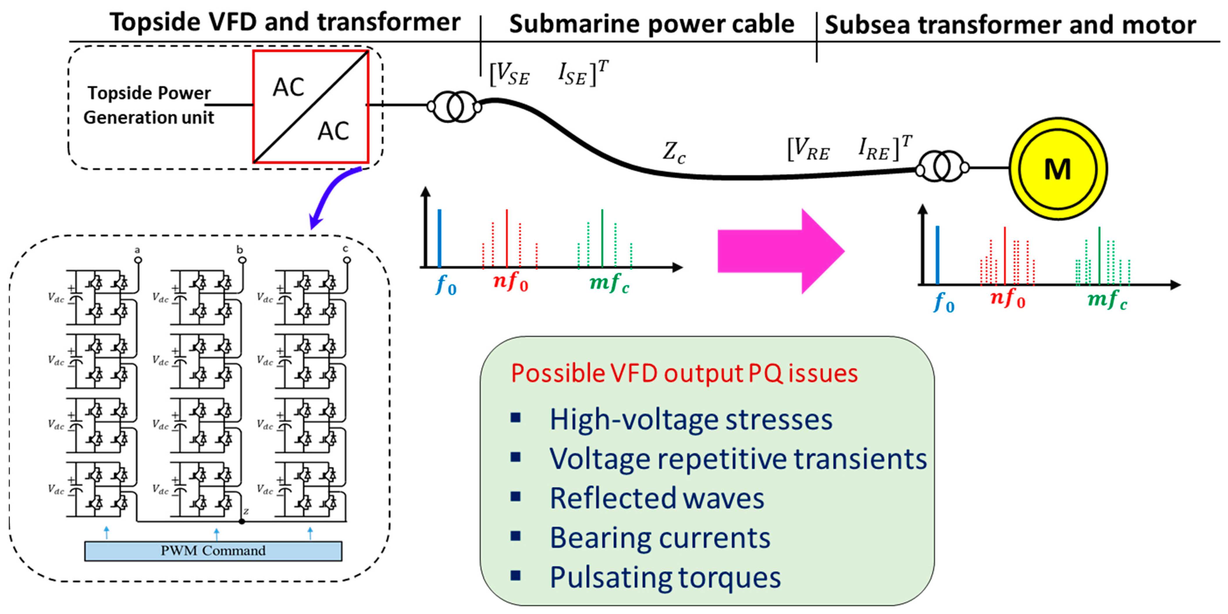
1.1.2. Power Quality Challenges to Operate ESP Systems with VFDs

Anxieties about repetitive ESP failures have been reported mainly due to high-voltage stress along the cable, which might have been magnified by its impedance [10,11]. Also, concerns about the torsional vibration phenomenon of rotating shaft systems have been continuously reported for several years from diversified ESP installations. The criticality of the issue varies from partial system failures to more severe failures, which may require the ESP system shutdown to avoid fatigue or harm to operators [12,13]. It is estimated that the retrieval and re-installation of cable, pumping equipment, and service costs can exceed USD 100 000 for ESP system failure [14]. In addition, premature failures are undesired as they result in repair or replacement costs outside the scheduled maintenance window, and they induce unwanted downtime resulting in loss of production.

Reports indicate that operators are experiencing productivity loss, potentially due to differential and common-mode harmonics, as well as other indirect effects stemming from poor voltage and current waveforms produced by the VFD [10,15]. Therefore, these issues must be addressed promptly to guarantee maximum performance and safety in the workplace. VFD voltage harmonics result from the modulation process utilized for controlling the power switches [16,17]. Figure 3 illustrates ESP systems’ common root cause failures resulting from poor power quality related to VFDs, including high-voltage stresses, repetitive voltage transients, reflected waves, common-mode harmonics, arcing currents, bearing currents, and pulsating torques [16]. The transmission line impedance can magnify VFD-generated harmonics if they are near line resonance modes. They create high-voltage stresses superposed to the regular system voltage along the cable and at the motor terminals. As a result, they can threaten the equipment insulation in a very short time [17]. It is crucial to take necessary precautions to minimize the voltage and current harmonics generated by VFD topologies, as they combine in the machine’s air gap, producing oscillating torque components, some of which may have high magnitudes [18]. If their frequencies are close to one of the shaft’s eigenfrequencies, there is a risk of excitation of the shaft’s eigenmodes, which could lead to mechanical shaft failures [19,20]. Therefore, it is imperative to ensure that these harmonics are minimized to prevent any potential failures [21].

To ensure the optimal performance of ESP systems, it is crucial to consider all possible factors that can trigger resonance modes. This includes hydrocarbon fluid velocity, gas slug, and sand in the wells, which is crucial. Neglecting any of these sources may lead to ineffective design and operation of the ESP systems. Therefore, it is imperative to consider all potential sources of resonance to ensure the efficient functioning of ESP systems [22,23,24]. In relation to VFD-generated harmonics, these power quality problems pose significant risks that may shorten the ESP run-life and potentially induce failures, which involve significant damage and downtime [22]. Therefore, an ESP system must be appropriately designed and operated to prevent costly failures and production downtime [23,24].

Unbalanced voltage and current are other electrical power-related issues that frequently degrade the performance and shorten the life of the three-phase ESP systems [25,26]. An unbalanced three-phase system can cause the ESP motor to experience poor performance or premature failure. Such risks are frequent in the specific case of a VFD-ESP system based on CHB multilevel inverter topology. For example, an unbalanced operation may result in at least one power cell, resulting from the failure of power semiconductors or any associated control equipment, such as gate drives, sensing devices, and control board [27]. This can lead to unbalanced VFD inverter output voltages and currents. The unbalanced voltages at the motor terminals cause a high unbalance of current, which can be 6 to 10 times larger than the voltage unbalance. Unbalanced currents induce high pulsating torque in the motor air gap, increase vibrations and mechanical stresses, and increase losses and motor overheating [26].

1.2. Motivations and Purposes

The ESP systems investigated in this paper have a pulse-width-modulated (PWM) inverter, a step-up transformer, an optional sinewave filter, a transmission line cable, and an induction motor coupled to a multi-inertia pump load. A successful ESP system integration requires complementary knowledge of rotor dynamics and VFDs operation and controls. The complexity of these topics may pose a challenge for field engineering teams when attempting to integrate them into their daily tasks. There is a need to understand the effects of VFDs on ESP’s operation and possibly link these effects to their runtimes. It is evident that knowledge of how mechanical harmonics are sent back to the VFD is also necessary. There are no well-defined acceptance design criteria to guide the engineering teams when analyzing power quality in ESP systems. There are no international standards for the quality of VFD output power delivered downhole to ESP motor to date.

In a CHB VFD-ESP system operating with faulty cells, the neutral-shift method can maximize the fundamental component of the output line-to-line voltages while keeping them balanced even if the line-to-neutral voltages remain unbalanced [27,28]. Such a goal is achieved by shifting the PWM reference phase voltage angles during the compensation mechanism. With such an approach, it is evident that the VFD output electric power spectrum is also shifted [28]. However, because the locations of the modified harmonics are unknown, it is crucial for the completeness of the design to analytically calculate these harmonics in the frequency domain, assess their effects on the power transmission line, and evaluate the type of pulsating torque components they are generating in the motor’s air gap [29,30].

1.3. Importance of This Investigation

Each investigated ESP system has a pulse-width-modulated inverter, a step-up transformer, an optional sinewave filter, a transmission cable, and an induction motor coupled to a multi-inertia pump load. Therefore, a system integration analysis should be performed to understand the system behavior before installation. However, simulating such a system takes time and effort. It requires complex skill sets to design, model, and implement in simulation software. Unfortunately, in the industry, such exercises can be troublesome for field engineers due to the complex nature of this activity. For field engineers designing and selecting ESPs, having some basic skills in performing high-level system analysis is advantageous. Additionally, understanding VFDs’ operation and control strategies can also be helpful. These skills may enable rigorously designed systems. This paper proposes an analysis technique to provide high-quality power supplied to a submersible pump system by a VFD.

It also explains how VFDs might excite mechanical-shaft torsional modes in such applications. The proposed model is an easy-to-use computer tool to replicate the steady-state behavior of low- and medium-voltage ESP systems under normal and abnormal operation modes, at different operating points, multiple cable cross-sections, short and long transmission distances, as well as low and high-power motors, combined with and without a sine filter. Engineers in charge of designing, selecting, integrating, and retrofitting ESP components and systems must have such tools for performing accurate power quality analysis.

Because ESP power quality is governed by the quality of the voltage produced by the VFD and the current circulating through the cable and the motor, voltage and current behavior along the system have been deeply analyzed. Analytical relationships of harmonics families produced by each VFD and their precise information in the frequency domain, accounting for inter-harmonics and common-mode oscillating components, are discussed. Double-Fourier voltage harmonics resulting from two-level, three-level NPC, and CHB multilevel inverters are graphically presented in the frequency domain for easy understanding. The outcomes are crucial for a robust system integration design to avoid catastrophic failures. The results are also crucial for torsional analysis. International standards require a torsional analysis to ensure the integrity of the rotating shaft in its entire operating range [29,30]. Consequently, the magnitude and frequencies of the pulsating torque components in the motor airgap are needed for such evaluation.

1.4. Mains Contributions

The key contributions provided in this investigation are:

• A comprehensive analytical description of resonance excitation phenomena in electrical and mechanical systems
• A simplified and unified method to build a general VFD model to mimic the output voltage of the two-level, three-level NPC, and CHB multilevel inverters.
• A theoretical categorization and the exact location of the families of harmonic frequencies at the output of each VFD topology.
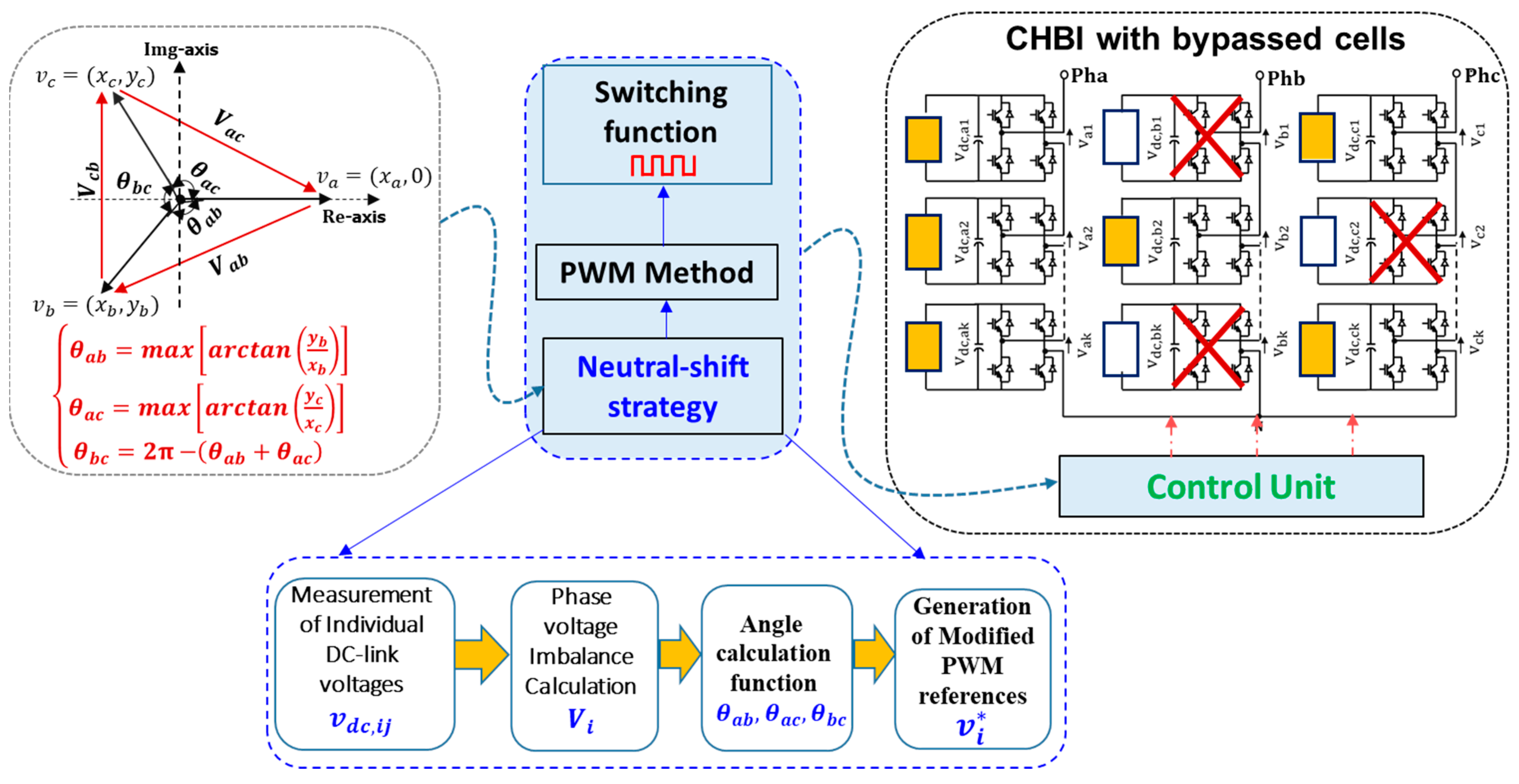
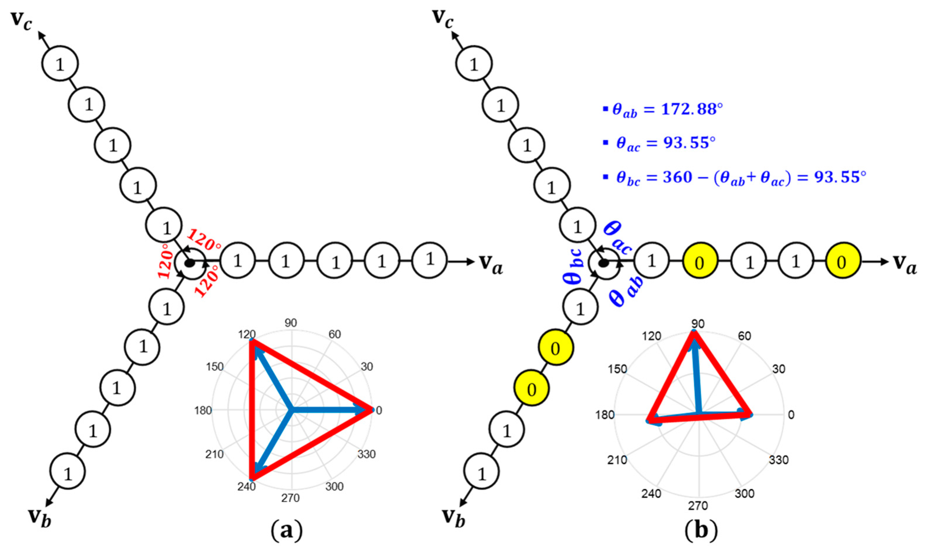
• An analytical assessment of the effects of the modified spectrum using the neutral-shift strategy with faulty cells on the electrical and mechanical systems.
• The theoretical foundations for calculating some key power quality parameters. The following PQ parameters are of particular interest:

  ○

  RMS and peak voltages and currents

  ○

  Maximum dv/dt

  ○

  Voltage and current THDs

Offline and real-time simulation results on different operating points support these theoretical contributions. Experimental test results on a reduced-scale laboratory setup are also provided and discussed to confirm the correctness of the suggested developments. For each simulated VFD-ESP system, voltage, current, and motor airgap torque harmonic components induced by each VFD topology are provided and correlated to theoretical predictions. The results are crucial for a robust system integration design to avoid catastrophic failures.

2. Modeling of Passive Components of ESP Systems

2.1. Basic Considerations

The investigated ESP system is illustrated in Figure 4. To investigate the electrical resonance modes, this system is simplified by its single-phase electrical model presented in Figure 5. As explained in Section 2.1, a controlled voltage source replicates the VFD. The transformer is modeled by its equivalent resistance and inductance, and the motor is replaced by its steady-state impedance [22]. The transmission cable is replaced by a set of pi-section networks (e.g., one per km). A pi-section is formed using lumped R, L, and C elements. The interconnection of multiple inertias constructs the rotating shaft system through stiffness constants and viscous damping elements. This section describes how rotating shafts and cables are modeled for mechanical and electrical resonance analyses.

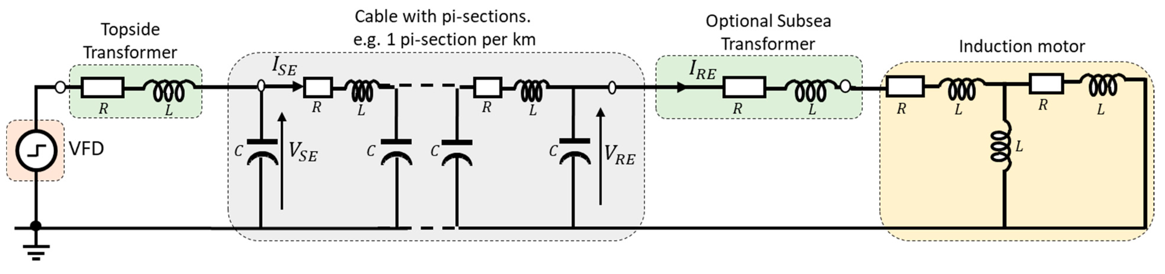
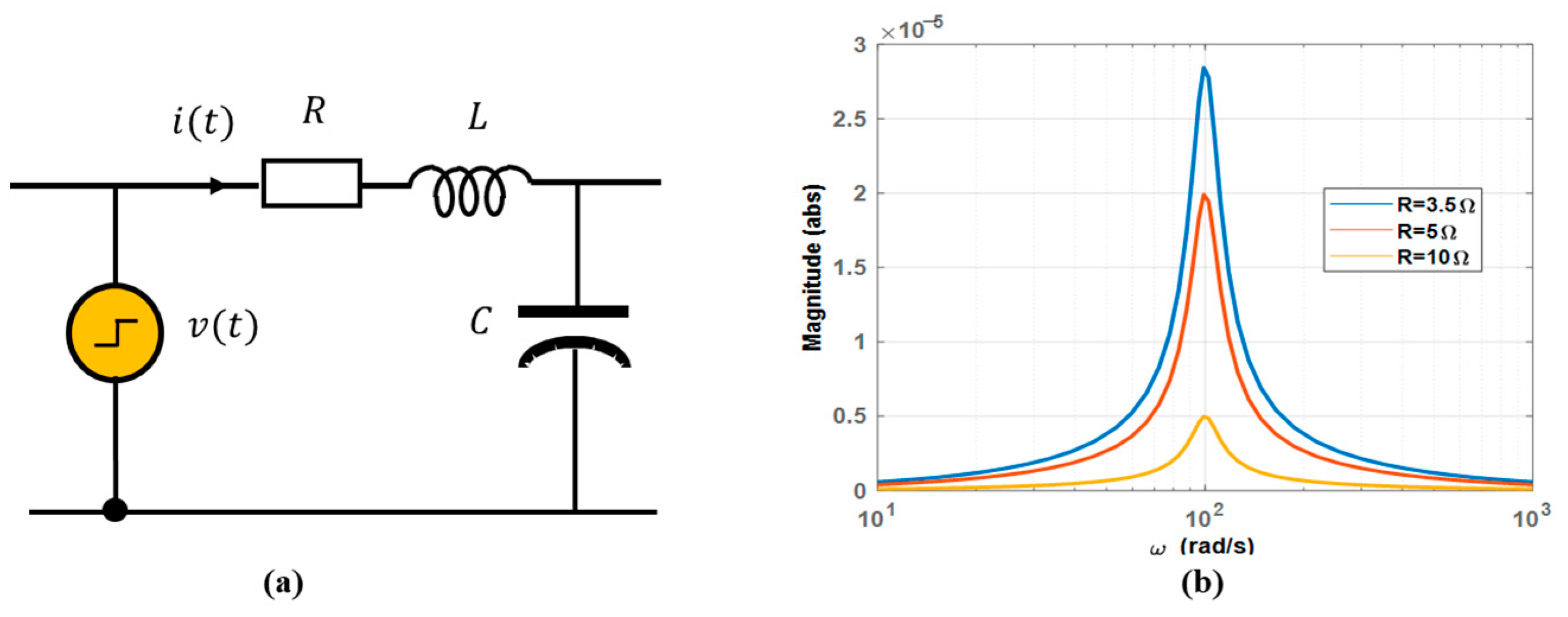
2.2. Transmission Line Cable

Figure 6a shows a series RLC circuit with a resistance R, an inductance L, and a capacitance C. Applying Kirchhoff’s voltage law to the circuit gives the following relationships:

$$L\frac{di\left(t\right)}{dt}+R.i\left(t\right)+\frac{1}{C}{\displaystyle \int }i\left(t\right)dt=v\left(t\right)$$

(1a)

$$\frac{d{i}^2\left(t\right)}{dt}+2n\frac{di\left(t\right)}{dt}+k^{2}i\left(t\right)=0$$

(1b)

$$n=\frac{R}{2L}$$

(1c)

$$k^2=\frac{1}{LC}$$

(1d)

With $k={\omega }_0$ being the circuit undamped natural frequency:

$$L{\omega }_0=\frac{1}{C{\omega }_0}=0\Rightarrow {\omega }_0=\frac{1}{\sqrt{LC}}$$

(2)

The relationship (1) is a second-order differential equation found in mechanical systems, as discussed in Section 2.2. Suppose the externally applied voltage $v\left(t\right)$ has a pulsating component near the undamped natural frequency ${\omega }_0$. In that case, $L$ and $C$ continuously exchange energy, such that the inductor transfers its energy to the capacitor, and the capacitor returns this energy to the inductor repetitively. Consequently, as shown in Figure 6b, for several values of R, only the resistance limits the current. This energy exchange creates a power oscillation; the current reaches its highest value at the resonance frequency.

As shown in Figure 5, the cable can be split such that each certain length, for example, each kilometer is represented by a pi-section, leading to multiple resonance frequencies. As a result, the voltage or current may reach very high values at those frequencies. The effects of load fluctuation can be analyzed with the same model. However, a current source replaces the motor model with multiple harmonics. Such analysis is suitable for understanding the effects of load dynamics (e.g., gas slugs) on the cable and its potentially destructive effects on the VFD.

2.3. Rotating Shaft System

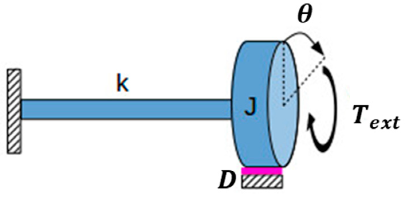
2.3.1. Basic Rotating Shaft with One Inertia

Figure 7 shows a system with a rotating inertia $J$, a damping factor $D$, and a stiffness $K.$ In addition, the shaft’s angular position is $\theta$.

The second Newton’s law applied to the system gives:

$$\frac{d{\theta }^2\left(t\right)}{dt}+2n\frac{d\theta \left(t\right)}{dt}+k^2\theta \left(t\right)=\frac{T_{ext}}{J},$$

(3a)

$$n=\frac{D}{2k}$$

(3b)

$$k^2=\frac{J}{K }$$

(3c)

A similarity is noted between Equations (1) and (3). When the damping of the rotating system is ignored and an external torque $T_{ext},$ oscillating at the system undamped natural frequency, is applied to the system, the following mathematical expressions can be formulated:

$$T_{ext}\left(t\right)=T_{a}sin\left({\omega }_{nat}t\right),$$

(4)

Thus, the coefficients in (3b) and (3c) are defined as follows:

$$n=0; k={\omega }_{nat}$$

(5)

The solution of (3a) is given as follows:

$$\theta \left(t\right)=\frac{T_a}{2{\omega }_{nat}}\left(\frac{1}{{\omega }_{nat}}\sin \left({\omega }_{nat}t\right)-tcos\left({\omega }_{nat}t\right)\right)$$

(6)

Equation (6) shows that if the shaft is driven by a torque component whose frequency is close to the undamped eigenfrequency, the shaft position oscillates at the same frequency with a 90° phase-shift and the following magnitudes:

• A constant value: $T_a/2{\omega }_{nat}{}^2$
• A linear time-varying value: $t\ast T_a/2{\omega }_{nat}$

As a result, the amplitude of the second component increases over time, even for small external torque magnitudes.

Figure 8 demonstrates the behavior of a system excited at its undamped natural frequency. For a system with a VFD, the external torque is the one inside the electric motor airgap. Therefore, VFDs must be designed to produce the machine’s electromagnetic airgap torque components with significantly small magnitudes near the shaft’s eigenfrequencies to prevent its excitation. For ESP applications, the mechanical torque during the process, like the induced by gas slugs, should be included in the shaft model because they are also generating electromagnetic torque components in the machine’s airgap.

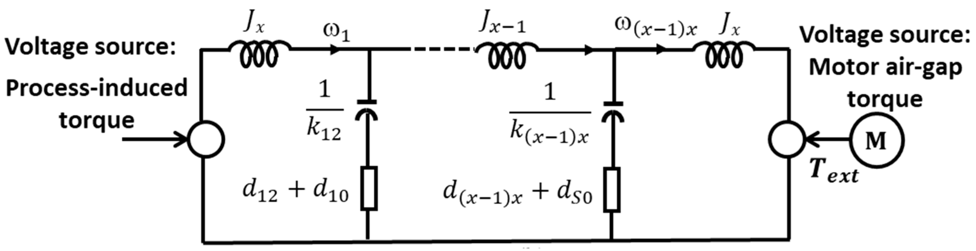
2.3.2. A Model of a Multi-Inertia Shaft System

A typical lumped-mass representation of the generator shaft is shown in Figure 9. A dynamic shaft model can be created using lumped parameters associated with the shaft elements. Such parameters, which include mass moments of inertia, damping coefficients, and stiffness constants between inertia, can be obtained by applying Newton’s second law [31], as demonstrated in Equation (7).

$$J\frac{d{\theta }^2\left(t\right)}{d{t}^2}+D\frac{d\theta }{dt}+K \theta =T_{ext}$$

(7)

where: $\theta$ is the vector of angular displacements of twists of individual disks to a common reference in radians. The matrix $J$ represents the mass moment of inertia, while $D$ is the damping factor matrix. $K$ is the stiffness matrix. The externally applied torque matrix is denoted by $T_{ext}$. These matrices play crucial roles in the dynamic analysis of mechanical systems. Therefore, understanding their properties and interrelations is essential for designing and optimizing such systems. With a base speed ${\omega }_b$, these matrices are given as follows:

$$J=\frac{2}{{\omega }_b}diag\left(J_1,J_2,\dots , J_x\right)$$

(8a)

$$T_{ext}={\left[T_1,T_2,\dots T_x\right]}^T$$

(8b)

$$\{\begin{array}{c}\begin{array}{l}{K}_{1,1} =k_{12}\hfill \\ K_{i,i} =k_{\left(i-1\right)i}+k_{\left(i-1\right)i}\hfill \\ K_{i,i+1}=K_{i+1, i}=k_{\left(i+1\right)i}=-k_{i\left(i+1\right)}\hfill \end{array}\\ K_{x,x}=k_{\left(x-1\right)x}\end{array}$$

(8c)

$$\{\begin{array}{l}{D}_{1,1}=d_{12}+d_{10}\\ D_{i,i}=d_{\left(i-1\right)i}+d_{\left(i+1\right)i}+d_{10}\\ D_{i,i+1}=D_{i+1,i}=d_{\left(i+1\right)i}=-d_{i\left(i+1\right)}\\ D_{x,x}=k_{\left(x-1\right)x}\end{array}$$

(8d)

where $i=2,3,\dots ,x-1$. The square roots ${\lambda }_i$ of the solutions to the characteristic equation are the undamped natural frequencies. ${\omega }_{nat,i}$ of the system:

$$\left[J^{-1}K-\lambda I\right]=0,$$

(9a)

$${\omega }_{nat,i}^2={\lambda }_i; i=1,2,\dots ,x$$

(9b)

where $I$ is a unity matrix. The system equations in (7) represent the shaft system dynamics. There are several other modeling approaches to represent the resulting equation of motion in the shaft system. Among these methods, the one based on its phenomenal equivalent electrical circuit model, as shown in Figure 10, is suitable for a torsional analysis [32].

According to the electromechanical phenological analogy, moments of inertia are equivalent to inductances, damping coefficients behave like electrical resistances, and the inverse of stiffness constants behave like electrical capacitors. Mechanical quantities also have their equivalent electrical quantities: angular velocity is equivalent to current, and torque to voltages.

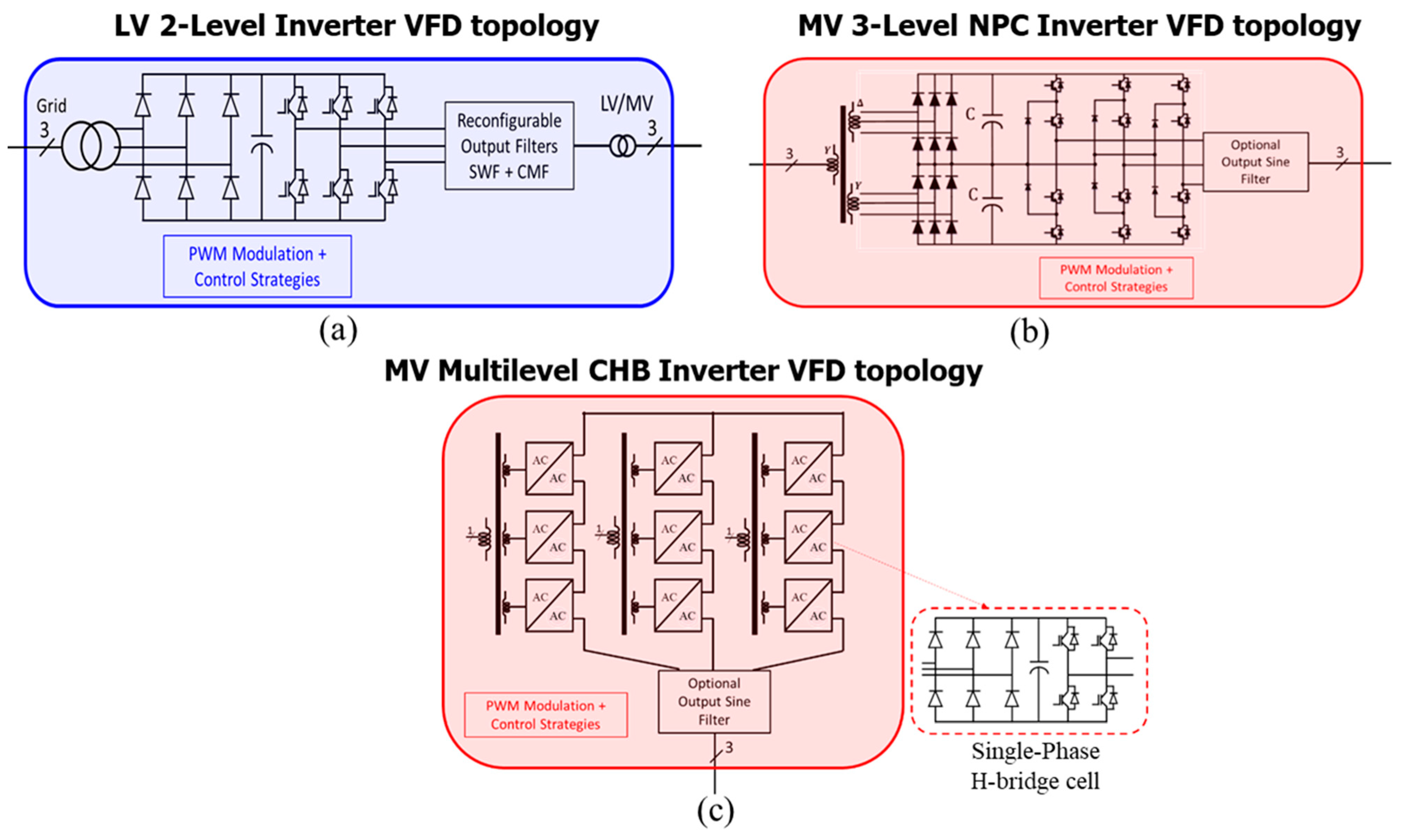
3. Modelling of VFD Topologies and ESP Motor for Torsional Analysis Purposes

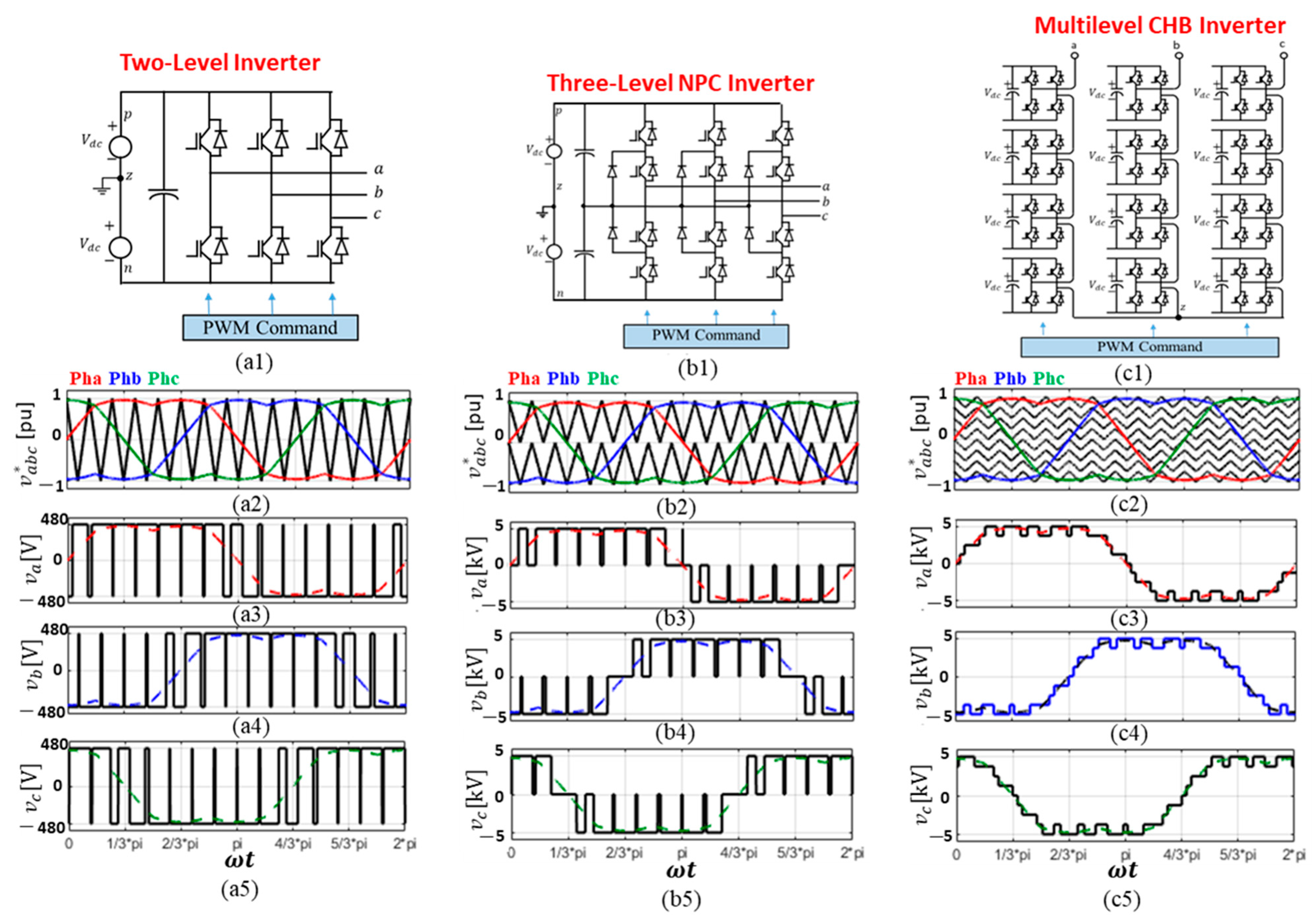
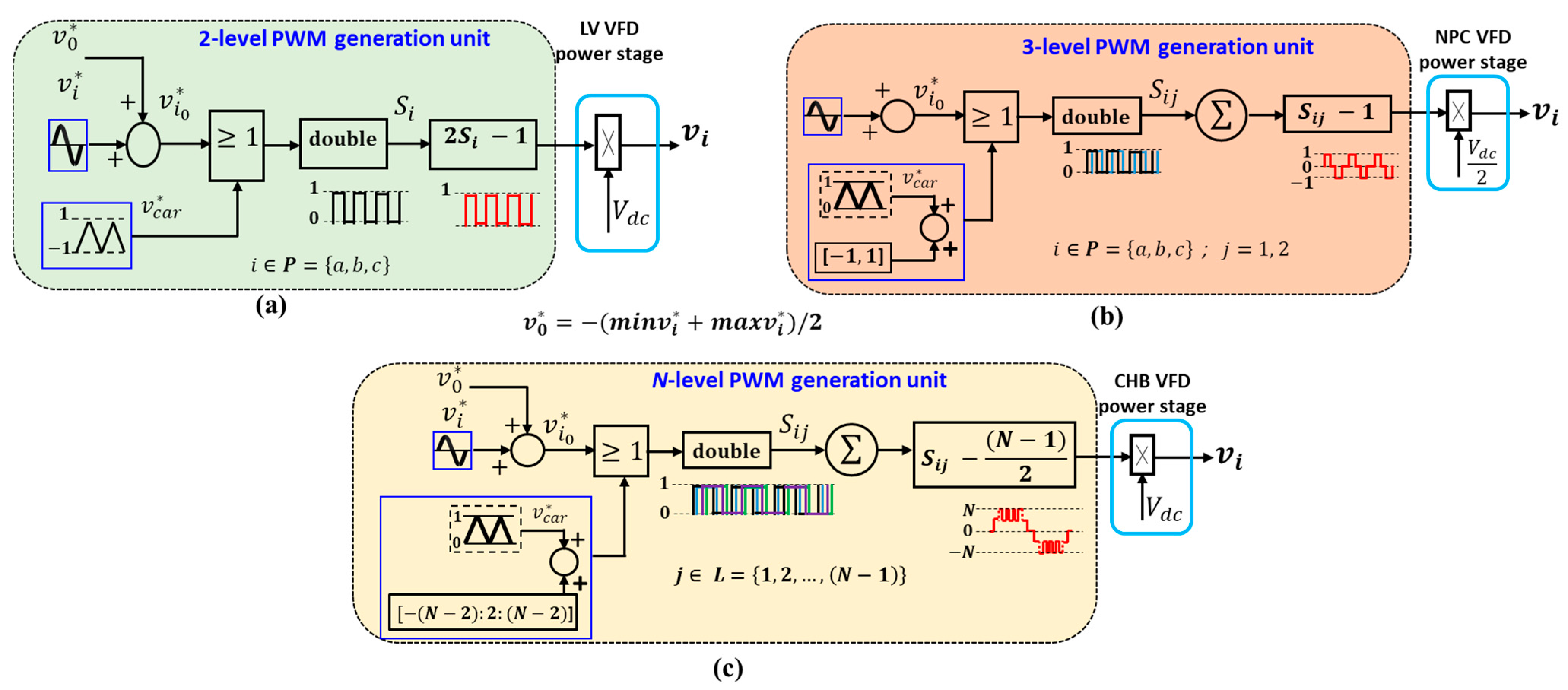
3.1. Time-Domain VFD Switching Function Models

Figure 11 shows different ways to control the output of VFDs using pulse-width-modulation that have been considered in this paper. Each VFD topology has its own unique modulation function. They include: (i) The low-voltage (LV) two-level inverter (Figure 11(a1)); (ii) The three-level NPC inverter (Figure 11(b1)), and (iii) The CHB multilevel inverter systems (Figure 11(a1)). The command strategy used is the sine-triangle PWM method. A sinusoidal reference wave is compared to one carrier signal per phase for the low-voltage two-level VFD, as shown in Figure 11(a2).

For the NPC and the multilevel CHB (N-level) VFD topologies, there are $N-1$ triangles in phase-disposition, as illustrated in Figure 11(b2,c2), respectively. Such disposition of carriers produces fewer harmonics compared to other multicarrier-based PWM techniques [33,34,35]. The modulated command creates a set of switched three-phase voltages from a constant or slowly varying DC-link voltage through a switching command function.

According to the above principle, the simplified switching function models two-level, three-level NPC, and $N$-level CHB inverters are shown in Figure 12a–c, respectively. Only one phase is shown; the other phases can be implemented by adding their respective references to the homopolar signal and comparing the results to the same carrier signals. A double-edge triangle carrier is compared to a reference voltage per phase. The average $(min,max)$ zero sequence or homopolar component $V_0$ is added into each reference phase voltage, such that the command pulses are equivalent to the space-vector PWM (SVPWM) pulses. A logic-to-real signal converter (“double” block) is used because the result of each comparator is a Boolean number. The generated modulated PWM signals create a set of switched voltages from a constant or slowly varying DC-link voltage through a switching command function. For a two-level VFD, $V_{dc}$ is the total DC-link voltage. A three-level NPC inverter uses only half of the total DC-link voltage. For an N-level model, each single power cell is supplied by a DC-link voltage that equals $V_{dc}$. Implementing the switching functions does not require an understanding of the detailed operating principle of a given VFD. Regarding the harmonic analysis, the control strategies (PID, vector controls) do not impact the system performance at steady states. Such an approach simplifies the numerical simulation of VFD topologies.

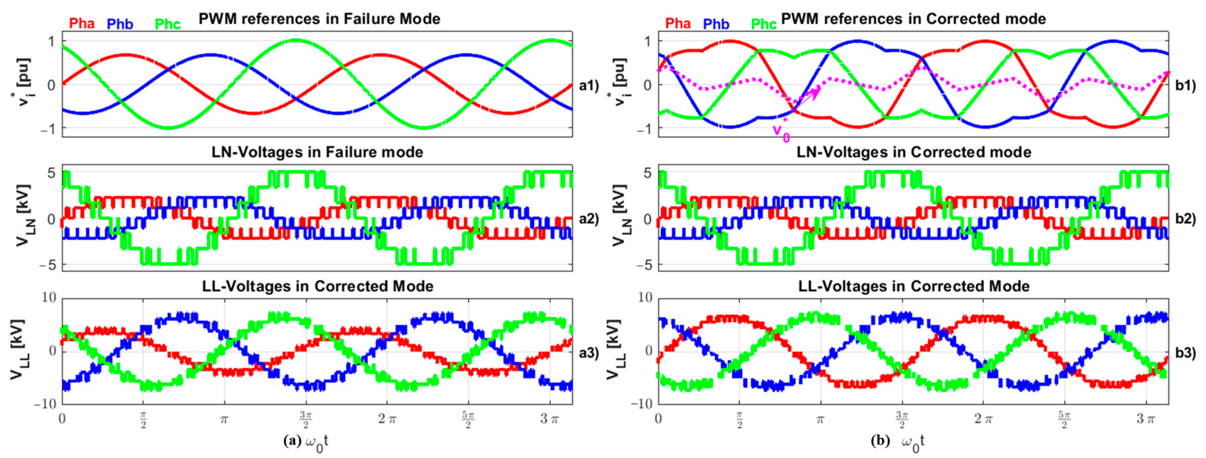
3.2. Neutral-Shift PWM Method in Cell-Fault Treatment for CHB Multilevel VFD Topology

The CHB multilevel inverter topology is a proven technology installed in several long tieback single-load pumping applications [36,37]. Because VFD availability and reliability are imperative in such applications, achieving acceptable performance with this type of VFD topology is very challenging. A common characteristic of this type of inverter is that many power semiconductors are required when output voltage levels increase [38,39]. With this increase in power semiconductor count, the fault probability of power cells also increases. Hence, the overall system’s reliability and efficiency decrease [40]. The most common faults that may occur in this topology are short- and open-circuit faults in power switches and the failures of their associated control boards. A failure of any component blocks the gate signals of the related power cell and bypasses its output. This leads to an unbalanced output voltage of the three-phase inverter, ultimately decreasing the system’s productivity.

The neutral-shift strategy is applied with faulty cells to maintain continuous safe system operation [28]. By adjusting the phase-shift angle between the reference phase voltages, the fictitious neutral of the inverter can be moved to ensure that balanced line-to-line voltages are generated by the VFD, even when dealing with unbalanced line-to-neutral voltages, as shown in Figure 13. Figure 14 shows voltage phasors for the two operation modes, normal operation mode (Figure 14a) and corrected mode (Figure 14b), with two failed cells in phases a and b using the neutral-shift method. Once the neutral-shift strategy is applied, the electrical harmonics generated by the VFD shift to different locations in the frequency domain. Consequently, they might threaten to excite the line’s electrical eigenfrequencies. Therefore, it is beneficial for the completeness of the design to track and quantify these harmonics to ensure the integrity of the system over the operational envelope. Double-Fourier voltage harmonics resulting from the CHB multilevel inverter under failed cells are graphically presented in the frequency domain in Section 3.

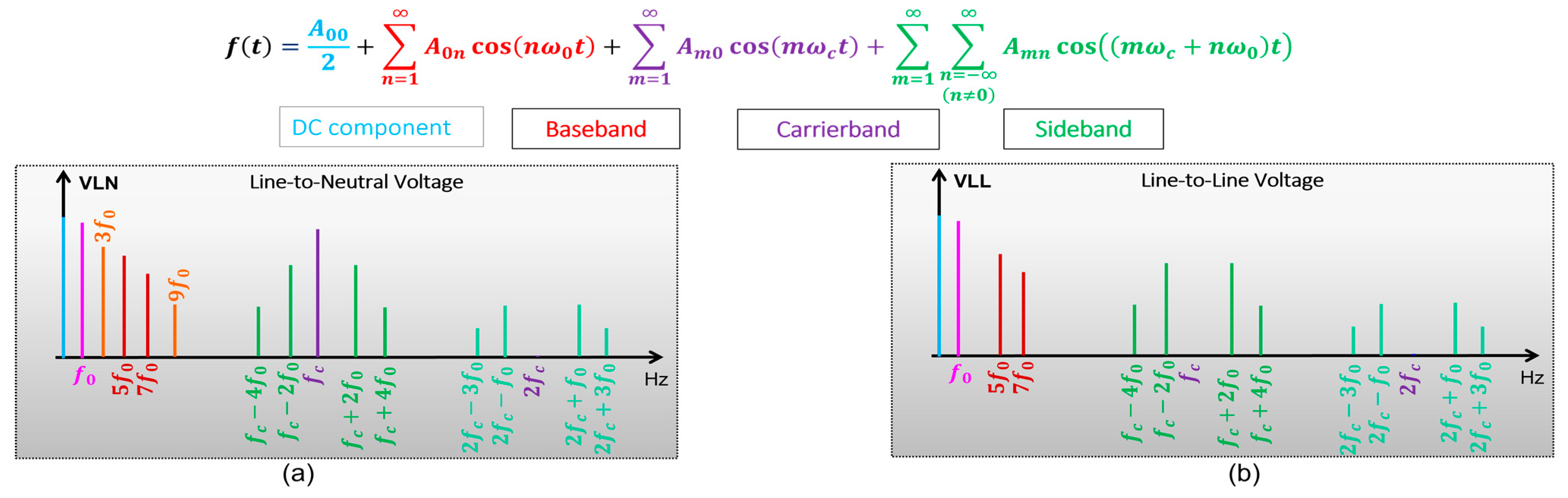
3.3. VFD-Induced Voltage Harmonic Families

This section provides detailed mathematical expressions of the harmonics at the output of each VFD topology discussed in Figure 11. These theoretical relationships are beneficial to understanding how each VFD creates high-frequency harmonic components that might excite the transmission cable and shaft system. In addition, they are needed to predict the location of the components in the frequency domain based on the VFD PWM’s carrier frequency and fundamental frequency.

3.3.1. A General Switching Function of a VSI-VFD

To mathematically formulate the switching function of each VFD in the steady state, the following assumptions are considered.

VFD power switch is turned on and off with no rise and fall times.

VFD DC-link is a constant DC-voltage.

The voltage drops across the switch, and leakage currents through the VFD switches are zero.

From a double Fourier transform, the analytical switching function of any carrier-based PWM strategy applied to any VSI power topology can be given as follows [35,36,37]:

$$s_{aVFD}\left(t\right)={\displaystyle \sum }_{m=0}^{\infty }{\displaystyle \sum }_{m=-\infty }^{\infty }{S}_{mn}cos\left(m{\omega }_{c}t+n{\omega }_{0}t+{\theta }_{mn}^v\right),$$

(10a)

$$v_{aVFD}\left(t\right)=S_{aVFD}\left(t\right)\ast V_{dc}$$

(10b)

where ${\omega }_c$ and ${\omega }_0$ are the PWM triangle carrier and the fundamental frequencies; ${\theta }_{mn}^v$ is the voltage harmonic phase-shift. $S_{mn}$ and ${\theta }_{mn}^v$ are expressions dependent on the implemented PWM method. Only phase voltages are calculated with respect to a common reference point, chosen as the DC-link’s mid-point. $m$ refers to the integer multiple of the carrier frequency, and $n$ to the multiple of the fundamental frequency. The set of integers $\left(m,n\right)$ is defined depending on the PWM strategy used [41]. Different harmonic families can be derived depending on their values, as indicated in Figure 15a [41].

The following electrical harmonic families can be found in all voltage source inverters:

• If $m=0$ and $n=0$, this corresponds to the DC component:
• If $m=0$ and $n=1$, this combination represents the fundamental voltage component.
• If $m=0$ and $n\succ 1$: this combination represents the baseband voltage harmonics. For three-phase systems, can only be given in the form of negative and positive sequence components, i.e., in the following form: $n=6l\pm 1$, with $l=1,2,3,\dots$
• If $m\ne 0$ and $n\ne 0$: this combination represents the sidebands or inter-harmonics [42,43]. They are arranged around carrier harmonic components and are visible when even values $m$ are paired with odd values of $n$ and vice versa. Therefore, sum $m$ + n should always be an even number, as shown in (11):

  $$m=2,4,6,\dots ; n=\pm 1, 3, 5$$

  (11a)

  $$m=1,3,5,\dots ; n=\pm 2, 4, 6$$

  (11b)

3.3.2. Analytical Switching Function of Investigated VFD Topologies

The analytical model of a two-level switching function is given in (12). Where $M$ is the modulation index such that $M=V_o/V_{dc},$ with $V_0$ the output peak voltage maximum

$$s_{a{z}_{\mathrm{LV}}}\left(t\right)=1+Mcos\left({\omega }_{0}t\right)$$

(12a)

$$+\frac{4}{\pi }{\displaystyle \sum }_{m=1}^{\infty }{\displaystyle \sum }_{m=-\infty }^{\infty }{S}_{mn}cos\left(m{\omega }_{c}t+n{\omega }_{0}t\right)$$

(12b)

The switching function expression of a three-level NPC inverter is given in (13):

$$s_{a{z}_{\mathrm{NPC}}}\left(t\right)=S_{01}cos\left({\omega }_{0}t\right)$$

(13a)

$$+{\displaystyle \sum }_{n=2}^{\infty }{S}_{0,2n-1}cos\left(\left(2n-1\right)n{\omega }_{0}t\right)$$

(13b)

$$+{\displaystyle \sum }_{m=1}^{\infty }{S}_{2m,0}cos\left(2m{\omega }_{c}t\right)$$

(13c)

$$+{\displaystyle \sum }_{m=1}^{\infty }{\displaystyle \sum }_{n=-\infty }^{\infty }{S}_{2\left(m-1\right),2n}cos\left(2\left(m-1\right){\omega }_{c}t+2n{\omega }_{0}t\right)$$

(13d)

$$+{\displaystyle \sum }_{m=1}^{\infty }{\displaystyle \sum }_{n=-\infty }^{\infty }{S}_{2m,2\left(n-1\right)}cos\left(2m{\omega }_{c}t+2\left(n-1\right){\omega }_{0}t\right)$$

(13e)

The mathematical model of the multilevel CHB VFD switching function is given(14):

$$s_{a{z}_{\mathrm{CHB}}}\left(t\right)=\frac{N-1}{2}{S}_{01}cos\left({\omega }_{0}t\right)$$

(14a)

$$+\frac{N-1}{2}{\displaystyle \sum }_{n=2}^{\infty }{S}_{0,2n-1}cos\left(\left(2n-1\right)n{\omega }_{0}t\right)$$

(14b)

$$+\frac{N-1}{2}{\displaystyle \sum }_{m=1}^{\infty }{S}_{2m,0}cos\left(2m{\omega }_{c}t\right)$$

(14c)

$$+\frac{N-1}{2}{\displaystyle \sum }_{m=1}^{\infty }{\displaystyle \sum }_{n=-\infty }^{\infty }{S}_{2\left(m-1\right),2n}cos\left(2\left(m-1\right){\omega }_{c}t+2n{\omega }_{0}t\right)$$

(14d)

$$+\frac{N-1}{2}{\displaystyle \sum }_{m=1}^{\infty }{\displaystyle \sum }_{n=-\infty }^{\infty }{S}_{2m,2\left(n-1\right)}cos\left(2m{\omega }_{c}t+2\left(n-1\right){\omega }_{0}t\right)$$

(14e)

3.3.3. Common-Mode Voltage Harmonics

The common-mode currents and voltages can cause harmful side effects in the ESP system, such as additional losses, reflected waves, bearing currents, insulation stress, and magnetic saturation. common-mode voltage $v_{CMV}$. represents the difference between the entire three-phase system and the neutral or the ground. The common-mode current $i_{CMV}$ travels in a single direction through all three wires, and it can only return to its source by using a different path, such as the neutral or ground, or perhaps parasitic components. Their mathematical expressions are shown in (15) and (16).

$$v_{CMV}\left(t\right)=\frac{v_{ag}\left(t\right)+v_{bg}\left(t\right)+v_{cg}\left(t\right)}{3},$$

(15)

$$i_{CMV}\left(t\right)=\frac{i_{ag}\left(t\right)+i_{bg}\left(t\right)+i_{cg}\left(t\right)}{3}.$$

(16)

A common-mode voltage harmonic component is a signal present simultaneously in all phases. Such quantity can be observed in phase-to-ground paths or any common reference point through either phase-to-ground or leakage impedance [44,45]. However, such a component is canceled through the differentiation of the phase voltages, which means it does not generate energy for the load. Also, it is not eliminated by a sine-filter, which is usually designed to cancel phase-to-phase harmonics only. A common-mode quantity is mathematically expressed as shown in (17):

$$v_{CMV}\left(t\right)=V_{CM{V}_k}cos(\lambda {\omega }_{k}t+{\varphi }_k),$$

(17a)

$$v_{ak}\left(t\right)=v_{bk}\left(t\right)=v_{ck}\left(t\right),$$

(17b)

where $k,\lambda$ are arbitrary integers, ${\omega }_k$ an arbitrary frequency, ${\varphi }_k$ an arbitrary phase-shift, and $V_{CM{V}_k}$ is the magnitude of the common-mode harmonic component. The quantities $v_{ak}$, $v_{bk}$, and $v_{ck}$ are the voltage of phases a, b, and c, respectively. In three-phase systems, all triplen baseband harmonics are common-mode quantities:

$$v_{ak}\left(t\right)=V_{CM{V}_k}cos(k{\omega }_{k}t) ,$$

(18a)

$$v_{ak}\left(t\right)=V_{CM{V}_k}cos\left(k{\omega }_{k}t\pm 2k\frac{\pi }{3}\right)$$

(18b)

$$v_{ak}=v_{bk}=v_{ck},\forall k=3h,h\in {\mathbb{N}}^{\ast }$$

(18c)

The modulation process is leading to the generation of common-mode voltage components for all VFD architectures under investigation. All carrier-band harmonics are, therefore, common-mode components. For VFD under investigation, these components are detailed in (19):

$$V_{CM{V}_{LV}}\left(t\right)=V_{dc}+V_{dc}{\displaystyle \sum }_{m=1}^{\infty }{S}_{m,0}cos\left(m{\omega }_{c}t\right)$$

(19a)

$$V_{CM{V}_{NPC}}\left(t\right)=V_{dc}{\displaystyle \sum }_{m=1}^{\infty }{S}_{2m,0}cos\left(2m{\omega }_{c}t\right)$$

(19b)

$$V_{CM{V}_{CHB}}\left(t\right)=V_{dc}{\displaystyle \sum }_{m=1}^{\infty }{S}_{\left(2m-1\right),0}cos\left(\left(2m-1\right){\omega }_{c}t\right)$$

(19c)

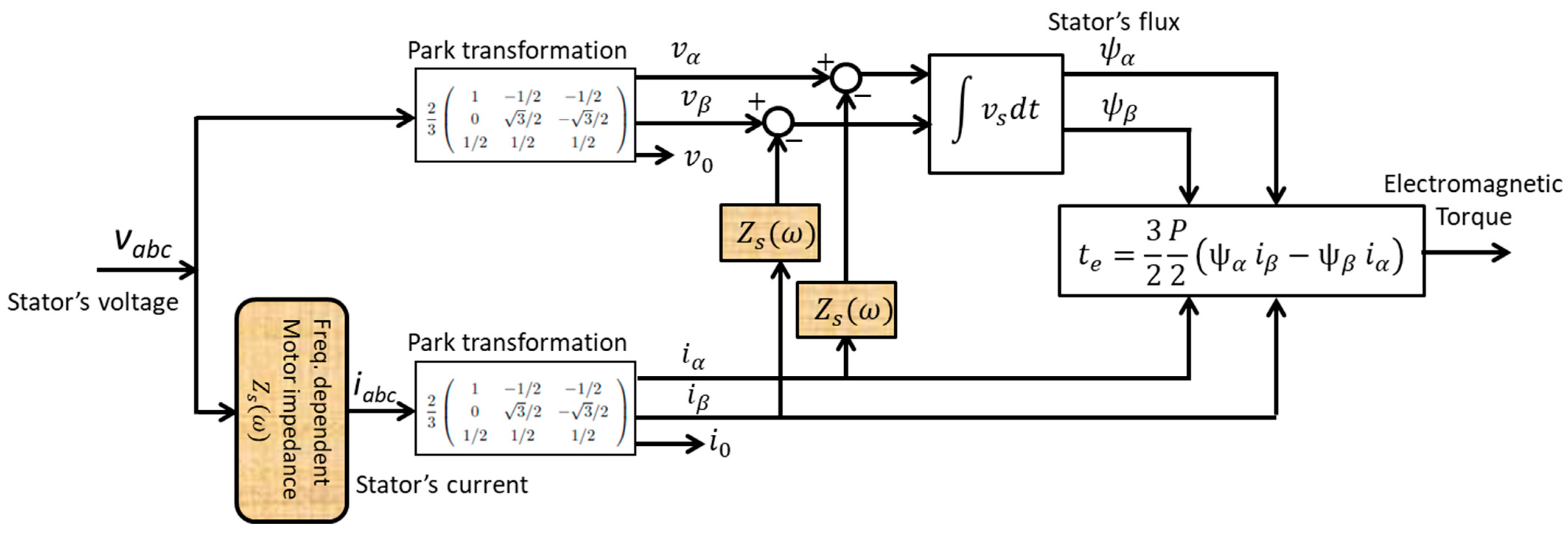
3.4. Modeling of ESP Motor Airgap for Torsional Analysis Purposes

The interaction between airgap torque harmonics and shaft system frequencies is challenging for VFD systems. Voltage and current harmonics from VFD topologies are combined in the airgap to create pulsating torque components, leading to excessive stress on the shaft. In addition, high-magnitude pulsating torques can result in mechanical shaft failures if they have frequencies close to the shaft’s natural frequencies. To ensure smooth and reliable operation of rotating machinery, it is crucial that VFDs are engineered in a way that minimizes torque components at the shaft’s undamped natural frequencies. This is essential to avoid any potential resonance excitation of the shaft and maintain optimal performance.

3.4.1. Electromagnetic Torque Time-Domain Model

The stator flux is defined as the time integral of the stator voltage, as mentioned in (20). For a P-pole motor (induction or synchronous), the electromagnetic torque in the ESP motor airgap is produced by the interaction of the motor stator flux and the current produced by the VFD.

$${\psi }_{abc}={\displaystyle \int }\left(v_{abc}-Z_s{i}_{abc}\right)dt$$

(20)

The torque is given in the stationary and orthogonal coordinates αβ [40]:

$$t_e\left(t\right)=\frac{3}{2}\frac{P}{2}\left({\psi }_{\alpha }{i}_{\beta }-{\psi }_{\beta }{i}_{\alpha }\right)$$

(21)

where $i_{\alpha }$ and $i_{\beta }$ are the currents in the $\alpha \beta$ reference, and ${\psi }_{\alpha }$ and ${\psi }_{\beta }$ are the stator fluxes in the αβ reference. Figure 16 shows the motor electromagnetic torque model that relies heavily on the stator’s voltages and currents’ quality [33]. The voltage drop due to the stator windings is neglected. It has a minor impact on the accuracy of the results because, in the frequency domain, the location of the torque components is not influenced by the impedance of the stator. Therefore, their magnitudes are slightly modified.

3.4.2. Analytical Formulation of VFD-Induced Torque Harmonic Components

Regardless of the operation mode of the ESP motor, voltage and current harmonic quantities in a steady state can be written in a generic form [19]:

$$v_a\left(t\right)={\displaystyle \sum }_{m_v=0}^{\infty }{\displaystyle \sum }_{n_v=0}^{\infty }{V}_{m_{v,}{n}_v}cos\left(m_v{\omega }_{c}t\pm n_v{\omega }_{0}t+{\theta }_{m_v,n_v}^v\right)$$

(22a)

$$i_a\left(t\right)={\displaystyle \sum }_{m_i=0}^{\infty }{\displaystyle \sum }_{n_i=0}^{\infty }{I}_{m_i,n_i}cos\left(m_i{\omega }_{c}t\pm n_i{\omega }_{0}t+{\theta }_{m_i,n_i}^i\right)$$

(22b)

where ${\omega }_c$ is the carrier frequency and ${\omega }_0$ the fundamental frequency; $m_v, n_v$ and $m_i,n_i$ are arbitrary integers; $V_{m_v{n}_v}$ and $I_{m_i{n}_i}$ are the voltage and current magnitudes. The arbitrary integer sets $\left(m_v, n_v\right)$ and $\left(m_i,n_i\right)$ depend on the VFD inverter topology and its modulation strategy. Equation (23) is an all-inclusive relationship that covers the complete spectrum of the instantaneous electromagnetic torque that can be produced by any VFD. It includes the DC-component (at 0 Hz); the baseband harmonics, which are integer multiple of the fundamental frequency, $n{\omega }_0$. And finally, the sideband components which are centered around an integer multiple of the carrier frequency, $m{\omega }_c+n{\omega }_0$.

$$t_e\left(t\right)={\displaystyle \sum }_{m=0}^{\infty }{\displaystyle \sum }_{n=-\infty }^{ \infty }{T}_{e,m,n}cos\left(m{\omega }_{c}t+n{\omega }_{0}t+{\theta }_{m,n}^{Te}\right)$$

(23)

The following airgap torque components and their sources of electrical (voltage and current) harmonic families are found in all investigated VFDs.

Airgap torque components from electrical fundamental and baseband harmonics

$$t_{e{z}_{0, 6n}}\left(t\right)=T_{eDC}+{\displaystyle \sum }_{n=0}^{\infty }{T}_e{}_{0,6n}cos\left(6n{\omega }_{0}t\right)$$

(24)

Airgap torque components from sidebands around even multiple of the carrier frequency of electrical harmonics

$$t_{e_{2m,\pm 2n}}\left(t\right)={\displaystyle \sum }_{m=1}^{\infty }{\displaystyle \sum }_{n=0 }^{\infty }{T}_e{}_{2m,6n}cos\left(2m{\omega }_{c}t\pm 6n{\omega }_{0}t\right)$$

(25)

Airgap torque components from sidebands around an odd multiple of the carrier frequency of electrical harmonics

$$t_{e_{2m,2n}}\left(t\right)={\displaystyle \sum }_{m=1}^{\infty }{\displaystyle \sum }_{\begin{array}{c}n=-\infty \\ \left(n\ne 0\right)\end{array}}^{\infty }{T}_e{}_{2m,2n-1}cos\left(\left[2m-1\right]{\omega }_{c}t\pm \left(2n-1\right){\omega }_{0}t\right)$$

(26)

A summary of possible locations of the airgap torque components induced by any VFD inverter topology in the frequency domain is given in

Table 1. Example of possible locations of the airgap torque oscillating frequencies.

Fundamental and Baseband Harmonics
$\left(\mathit{m},\mathit{n}\right)$	Voltage/Current	Torque
$\left(\mathbf{0}, \mathbf{1}\right)$	${\omega }_0$	$0$
$\left(\mathbf{0}, \mathbf{5}\right)$	$5{\omega }_0$	$6{\omega }_0$
$\left(\mathbf{0}, \mathbf{7}\right)$	$7{\omega }_0$
$\left(\mathbf{0}, \mathbf{11}\right)$	$11{\omega }_0$	$12{\omega }_0$
$\left(\mathbf{0}, \mathbf{13}\right)$	$13{\omega }_0$
Carrier band and sideband harmonics around odd multiple of carrier frequency
$\left(\mathbf{1}, \mathbf{0}\right)$	${\omega }_c$	None
$\left(\mathbf{1}, \mathbf{2}\right)$	${\omega }_c\pm 2{\omega }_0$	${\omega }_c\pm 3{\omega }_0$
$\left(\mathbf{1}, \mathbf{4}\right)$	${\omega }_c\pm 4{\omega }_0$
$\left(\mathbf{1},\mathbf{6}\right)$	${\omega }_c\pm 6{\omega }_0$	None
$\left(1, 8\right)$	${\omega }_c\pm 8{\omega }_0$	${\omega }_c\pm 9{\omega }_0$
$\left(\mathbf{1}, \mathbf{10}\right)$	${\omega }_c\pm 10{\omega }_0$
Carrier band and sideband harmonics around even multiple of carrier frequency
$\left(\mathbf{2}, \mathbf{0}\right)$	None	None
$\left(\mathbf{2}, \mathbf{1}\right)$	$2{\omega }_c\pm {\omega }_0$	$2{\omega }_c$
$\left(\mathbf{2}, \mathbf{3}\right)$	$2{\omega }_c\pm 3{\omega }_0$	None
$\left(\mathbf{2},\mathbf{5}\right)$	$2{\omega }_c\pm 5{\omega }_0$	$2{\omega }_c\pm 6{\omega }_0$
$\left(\mathbf{2},\mathbf{7}\right)$	$2{\omega }_c\pm 7{\omega }_0$
$\left(\mathbf{2},\mathbf{9}\right)$	$2{\omega }_c\pm 9{\omega }_0$	None
$\left(\mathbf{2},\mathbf{11}\right)$	$2{\omega }_c\pm 11{\omega }_0$	$2{\omega }_c\pm 12$
$\left(\mathbf{2},\mathbf{13}\right)$	$2{\omega }_c\pm 13{\omega }_0$

.

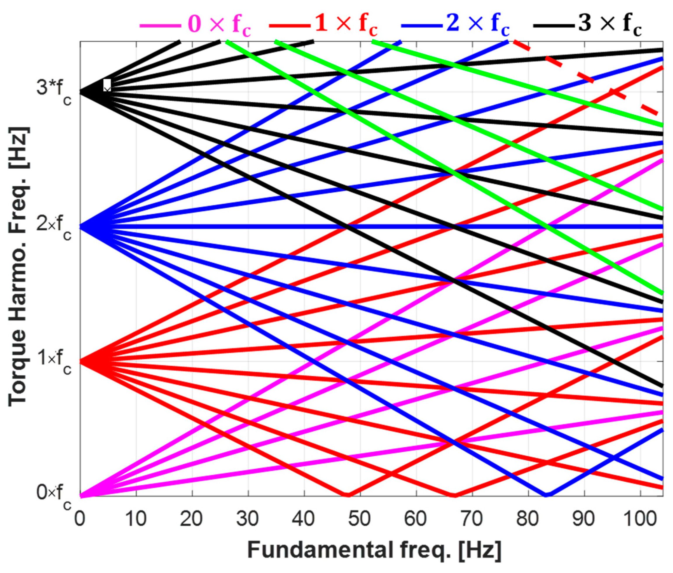
3.4.3. Family of Campbell Diagram Lines for VFD-Induced Pulsating Torque

This section provides the theoretical foundations to plot Campbell diagrams of ESP motors supplied by VFD topologies for torsional analysis. Such diagrams show the location of electromagnetic airgap torque component frequencies for the entire speed range. They are required by the API 617 standard [23] to evaluate the shaft’s ability to withstand stresses through the entire speed range of the motor. Theoretical lines of the Campbell diagram are derived from the expression of the torque harmonic frequencies, given in [19]:

$${\omega }_h=\left(m_i-\frac{{\epsilon }_{n_i}}{{\epsilon }_{n_v}}{m}_v\right){\omega }_c\pm \left(n_i-\frac{{\epsilon }_{n_i}}{{\epsilon }_{n_v}}{n}_v\right){\omega }_0$$

(27)

Only a few of the components in (38) are relevant for a torsional analysis. Meaningful lines are derived based on the importance of their respective torque magnitudes. For a combination of arbitrary integer sets $\left(m_v, n_v\right)$ and $\left(m_i,n_i\right)$, the torque magnitude is given in (28).

$$T_{eh}={\epsilon }_{n_v}\ast \frac{3}{2}\frac{P}{2}\frac{V_{m_v,n_v}}{m_v{\omega }_c\pm n_v{\omega }_0}{I}_{m_i,n_i}$$

(28)

Consequently, $T_{eh}$ has a significant value for $m_v=0$. Also, the product $V_{m_v{n}_v}\ast I_{m_i{n}_i}$ has a significant value when at least one of them is the fundamental component. Therefore, the relevant torque magnitudes should be derived as follows: (i) The fundamental current component, $m_i=0, n_i=1$, should be combined with the baseband voltage harmonics, i.e., $m_v=0, n_v>1$. (ii) Only the fundamental voltage component, $m_v=0, n_v=1$, should be combined with all current harmonics. The possible meaningful magnitudes are summarized in (29):

$$T_{eh}=\frac{3}{2}\frac{P}{2}\frac{V_{0,n_v}}{n_v{\omega }_0}{I}_{0,1}$$

(29a)

$$T_{eh}=\frac{3}{2}\frac{P}{2}\frac{V_{0,1}}{{\omega }_0}{I}_{m_{i,}{n}_i}$$

(29b)

The frequencies of components having relevant magnitudes for torsional analysis are as follows: (i) For $\left(m_i, n_i\right)\in \left(0, 1\right)$, then $m_v=0$ for all $n_v>1$; (ii) For $\left(m_v, n_v\right)\in \left(0, 1\right)$ $m_v=0, n_v=1$, for all combinations of $m_i, n_i.$ Thus, the frequencies that appear in the Campbell diagram are given in (30):

$${\omega }_h=\left(n_v\pm 1\right){\omega }_0$$

(30a)

$${\omega }_h=\left|m_i{\omega }_k\pm \left(n_i\pm 1\right){\omega }_0\right|$$

(30b)

Equation (30) is the only relationship needed to plot a complete Campbell diagram and extract the torque magnitudes required for the torsional analysis. Lines generated from (31a) are called baseband lines, and the ones from (31b) are sideband lines [46]. Figure 17 shows a generic Campbell diagram for PWM-VFDs based on Equation (30), with a given carrier-frequency $f_c$. The stator’s frequency range is from 0 to 105 Hz.

4. Power Quality Parameters Calculation

4.1. Key Parameters to Characterize the Quality of Power in ESP Systems

Poor VFD output power quality is the cause of many electrical failures in ESP systems [11,47,48,49]. Therefore, attention is paid to the quality of voltages and current delivered downhole to the ESP motor. The quality of power can be evaluated through a set of performance factors. By quantifying the profile of power quality supplied to the ESP motor, the user can clearly understand the impact of these factors on the quality of power supplied to the ESP motor. This section provides the theoretical foundations for assessing key power quality parameters in ESP systems supplied by VFDs. The following parameters are of particular interest:

• RMS and peak voltages and currents
• Maximum dv/dt
• Voltage and current THDs
• Common-mode voltage and current

These parameters are discussed in this paper for pedagogical purposes only. However, the common-mode quantities are discussed in dept to analytically clarify their origins through the PWM modulation process applied to the three VFD topologies under investigation.

4.2. RMS and Peak Voltages and Currents

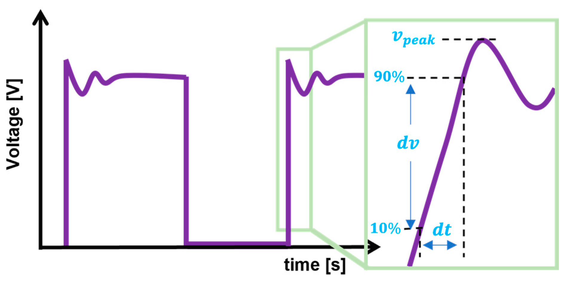
A quantity’s RMS (root-mean-square) value is a mathematical expression used to find its effective value. It is the square root of the average of the squares of the values over a given period. It is the measurement used for any time-varying signal’s effective value. The peak value is the maximum instantaneous value of a signal as measured from zero-level.

Take a sine wave representing either voltage or current with peak $y_{peak}$:

$$y\left(t\right)=y_{peak}sin\left(\omega t\right)$$

(31)

the RMS value $y_{RMS}$ is given by:

$$y_{RMS}=\sqrt{\frac{1}{T}{{\displaystyle \int }}_0^T{y}^2\left(t\right)dt}=\sqrt{\frac{1}{T}{{\displaystyle \int }}_0^T{A}^2{sin}^2(\omega t)dt } \approx y_{peak}/\sqrt{0.7}$$

(32)

4.3. Maximum dv/dt

When looking at voltage waveforms generated from VFDs, they may appear to be square at first glance. However, upon a closer inspection at the leading edge of the pulse, the rise-time of the pulse becomes noticeable. The change in voltage, noted “dv”, and the change in time, noted “dt”, is utilized to compute the voltage gradient, dv/dt, as illustrated in Figure 18. The rise time (t_r), shown as dt, is the time required for the voltage to travel from 10% to 90% of its peak value. The dv/dt is the slope of the voltage rise in volts per microsecond. It can be approximately computed as 80% of the peak voltage divided by the rise time. High dv/dt due to short rise times may create voltage spikes at the leading edge of the voltage pulse. Voltage spikes can create ringing effects because of the cable impedance, potentially leading to higher voltage stresses on the system insulation [47].

$$\frac{dv}{dt}=\frac{0.8\ast V_{peak}}{t_r},$$

(33)

In calculating dv/dt, refer to NEMA Standard MG1 [48]. The rise time may be influenced by the switching characteristics of the VFD power switches (such as IGBTs and MOSFETs) and other related components. Additionally, other factors in the VFD circuit can impact the rise time and the height of the overshoot. They include:

• The snubber circuit design;
• The internal impedance of all the components between the DC-link voltage and the output of the VFD;
• The wiring and connection components in the power circuit

The first generation of IGBTs had a larger riser time (about $2.5 \mathsf{\mu }\mathrm{s})$. Some of these devices can still be found in installed ESP systems. However, newer IGBTs have been designed with a lower rise time (about $0.1 \mathsf{\mu }\mathrm{s}$), which may be found in most new VFDs for ESP applications [48].

4.4. Voltage and Current Total Harmonic Distortion

The total harmonic distortion (THD) of a signal refers to the level of distortion in a waveform caused by the presence of harmonics. It measures the extent to which harmonics have altered the original waveform. As described in Section 3, the harmonic frequencies of a voltage or current are frequency components in the signal at an integer multiple of the frequency of the fundamental component (baseband components), and components that are the combination of switching and fundamental frequencies, called sidebands harmonics or inter-harmonics. THD is defined as [48]:

$$THD(\%)=100\times \frac{\sqrt{{{\displaystyle \sum }}_{k=2}^{\infty }{V}_{k,RMS}^2}}{V_{1,RMS}},$$

(34)

where, $V_{k,RMS}$: is the RMS voltage of the kth harmonic and $V_{1,RMS}$: is the RMS voltage of the fundamental frequency. Equation (34) shows the mathematical definition of THD; The voltage is used in this equation, but current could be used instead.

5. Offline Numerical Validations

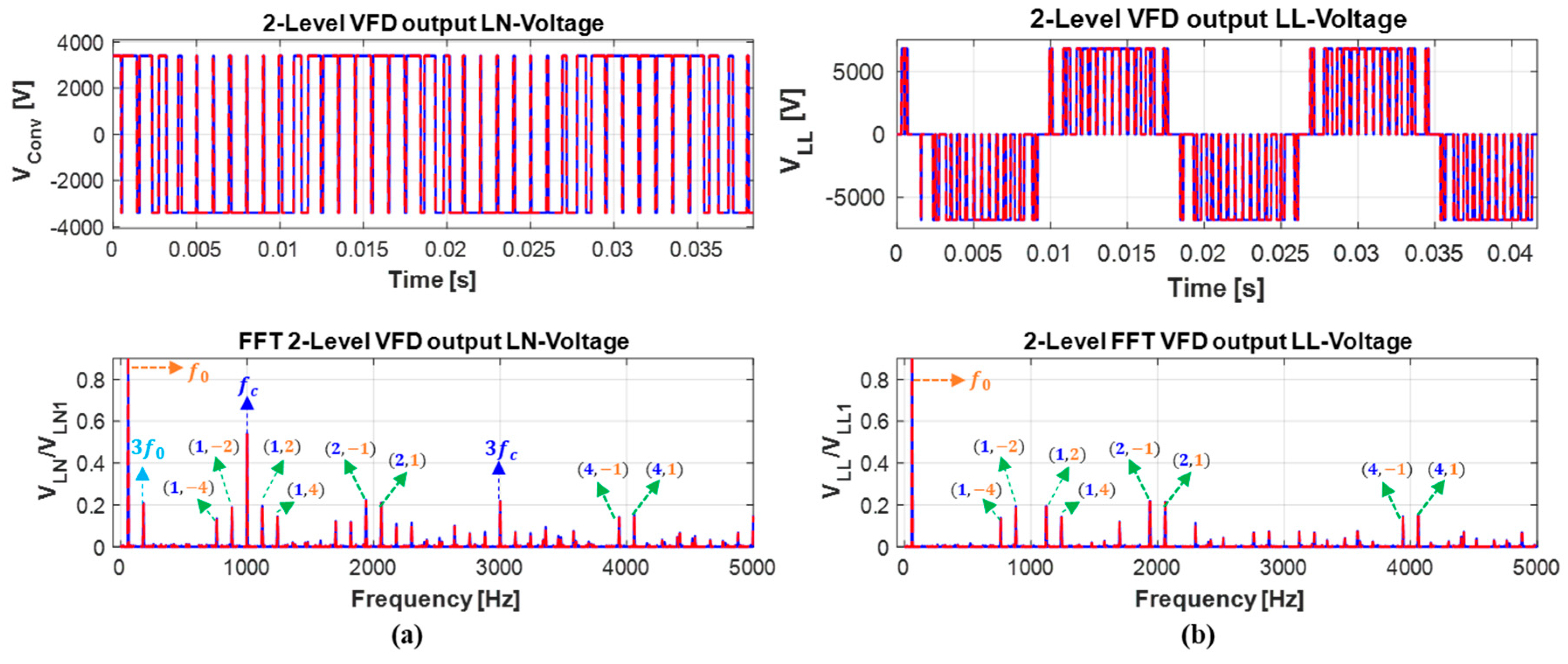
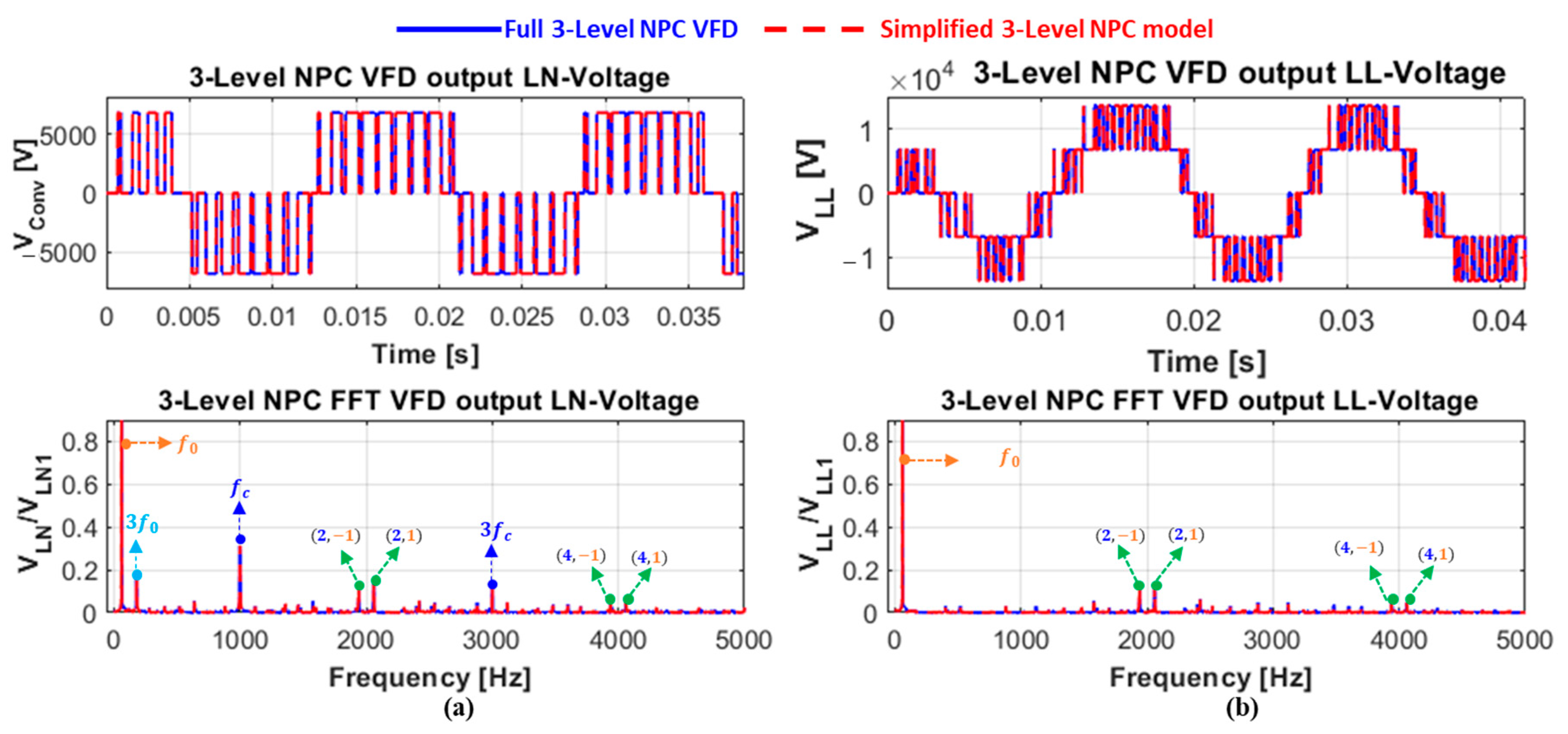
5.1. Numerical Validation of VFD Switching Function

Selected time and frequency domain simulation results from the two-level VFD switching models are shown in Figure 19, where the inverter line-to-neutral and line-to-line voltages waveforms are illustrated. Similar simulation comparison results in both time and frequency domains are shown in Figure 20 and Figure 21 for a three-level NPC VFD and seven-level CHB VFD, respectively. The results from the simplified model (dotted red line) are superposed to the ones obtained from the complete VFD topology (straight blue line) with the entire PWM strategy and the inverter’s power stages with IGBTs. In all the simulated cases, both models’ generated voltage waveforms accurately match. The resulting spectra show a good fit between each VFD topology and its simplified model, where their generated harmonic components are located at similar frequencies with matching magnitudes. As the levels of output voltage increase, the output power quality is improved. The seven-level CHB VFD produces less harmonic distortion than the three-level NPC, which in turn shows fewer harmonic components than the two-level VFD at the same operating frequencies and same carrier frequencies. Therefore, the locations of VFD output voltage harmonic components are consistent with theoretical calculations. In all the simulated cases, LN-voltages generated by each VFD produce three families of harmonics: baseband components which are proportional to the fundamental motor frequency; sideband or inter-harmonic components around the carrier frequency; and common-mode harmonics, which are triple baseband and carrierband components. All these common-mode harmonic components are seen canceled through the differentiation of the LL-voltages generated by each VFD topology.

The simplified VFD model provides high flexibility to perform VFD output power quality analysis with a wide range of operating conditions at reduced computation time. Double-Fourier voltage harmonics resulting from two-level, three-level NPC, and CHB multilevel simplified models with the fundamental frequency varying from 35 Hz to 60 Hz, with a step of 5 Hz, are graphically presented in Figure 22.

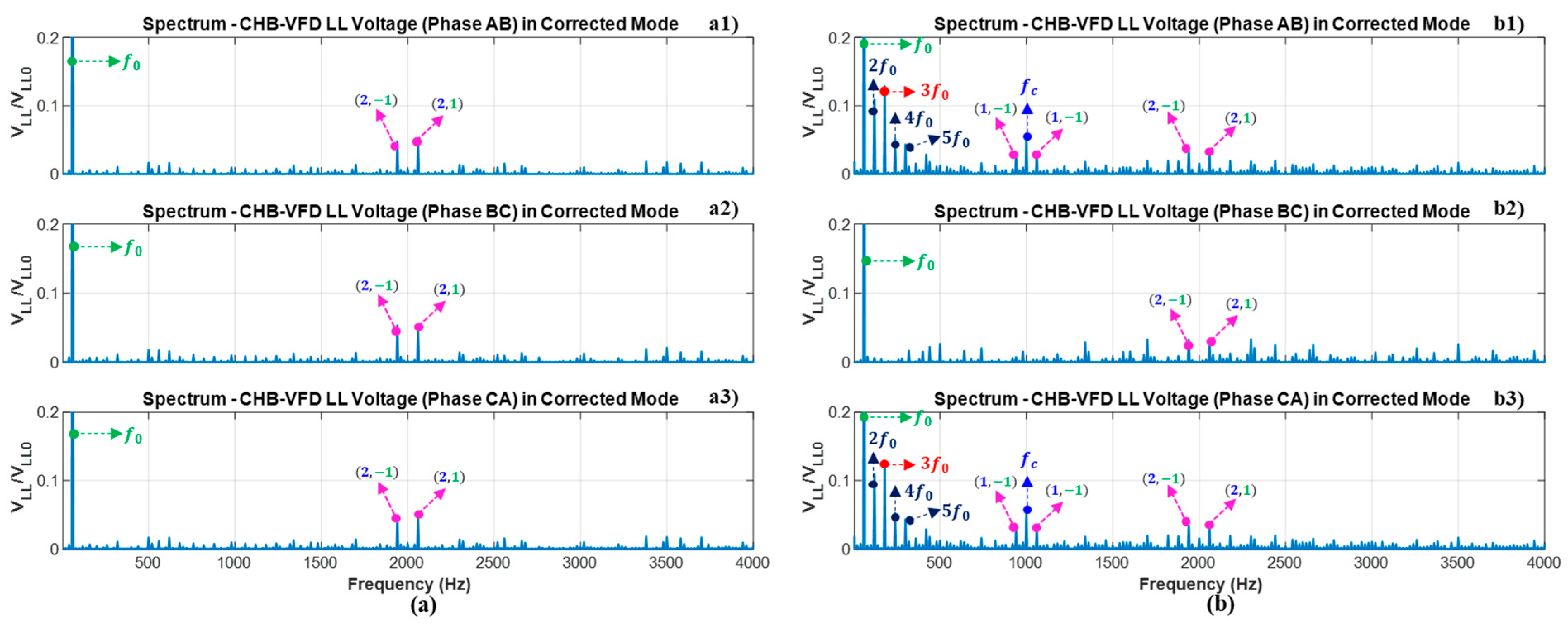
5.2. Selected Simulation Results of CHB VFD with Failed Cells

Figure 23 shows the selected time domain results of a CHB VFD inverter (k = 3 H-bridges per phase) with two failed and bypassed cells in phase A. The voltage vector per phase discussed in this case is given by: vdc, a = [0 0 1]; vdc, b = [1 1 1]; and vdc, c = [1 1 1]. The failure of two H-bridge cells results in a decrease of two levels in the waveform of VA, as shown in Figure 23(a2), leading to an unbalanced line voltage when any correction method is applied, as shown in Figure 23(a3). The neutral shift-based compensation method produces balanced output line voltages even if inverter phase voltages remain unbalanced. The PWM reference voltages’ phase angles have been modified by the theory outlined in Section 3.2. Instead of the normal 120°, the inverter’s phase A is displaced from phases B and C by 140.4°. Under corrected mode, the CHB VFD inverter with failed cells generates a three-phase balanced line voltage, unfortunately with higher harmonic distortion, as discussed in Figure 24 and Figure 25.

Figure 24 depicts the harmonic spectrum analysis of the generated phase voltage in both normal and corrected modes. As can be observed in Figure 24(b1), phase A’s failure of two power cells has led to higher harmonic distortion than under normal conditions (Figure 24(a1)). It can be observed that additional undesired harmonic components appear around the multiples of THE fundamental frequency, $f_0$, on the output voltage of CHB-VFD, such as $2f_0,$ $4f_0, 5f_0, 6f_0$ and so on. It also observed a significant rise in sideband harmonic components around $f_c$ and 2$f_c$. The spectra of phase voltages $V_B$ (Figure 24(b2)) and $V_C$ (Figure 24(b3)) are not altered and remain the same as under normal conditions since only phase A is affected. The spectrum quality of line voltage $V_{Bc}$(Figure 25(b2)) has not been impacted and is the same as under normal conditions. In contrast, because they result from the differentiation with phase A, the spectrum of line voltages $V_{AB}$ (Figure 25(b1)) and $V_{AC}$ (Figure 25(b3)) are identically altered.

It is essential to highlight that the common-mode harmonics are the triplen baseband (e.g., 3$f_0$) and the carrierband components (e.g., $f_c, 2f_c$) in normal conditions. They are no longer common-mode harmonic components in faulty conditions. As can be observed in Figure 25(b1,b3), they are not canceled through the differentiation of the LL-voltages. These results are crucial for a robust engineering system integration design to avoid catastrophic system failures resulting from possible VFD-induced resonance excitation of the transmission-line electrical, natural frequencies.

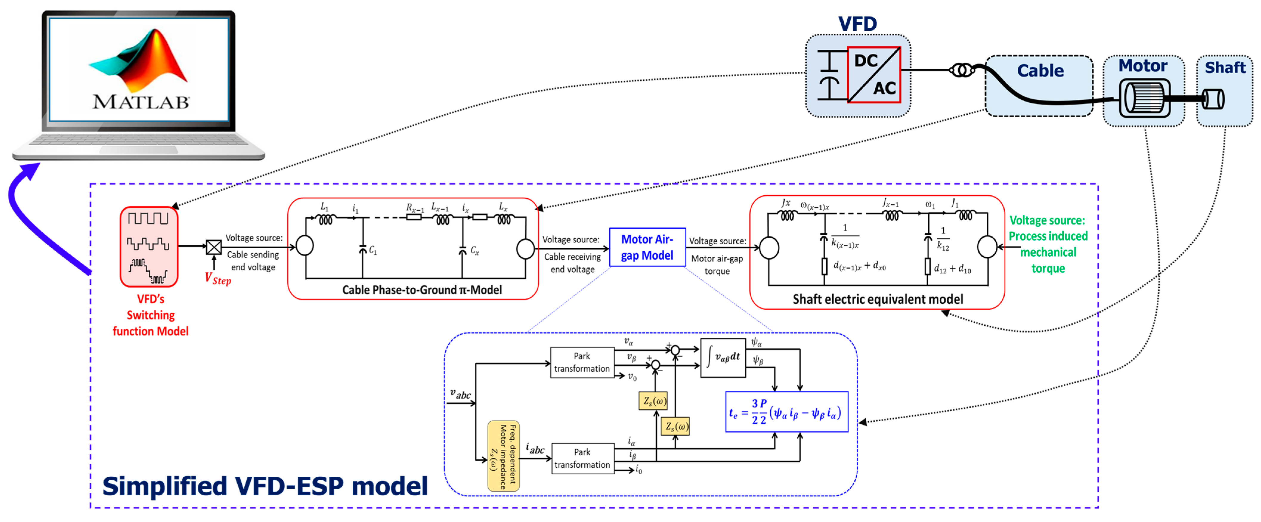
5.3. Implementation and Simulation of the Overall VFD-ESP System Models

5.3.1. Simulated VFD-ESP System Model and Validation Principle

The closed-form time and frequency domain models of VFDs developed in the previous section are crucial to understanding the location of voltage harmonics generated and analyzing their propagation along the transmission cable and motor terminals. Once the closed-form VFD models are known, the VFD power stage configurations, including IGBTs, are not needed anymore for the overall ESP system simulation and analysis. Because ESP power quality is governed by the quality of the voltage generated by the VFD and the current flowing through the system, the behavior of the voltage and current applied at the motor terminal is analyzed in this section. The integrated equivalent simplified model of the overall ESP system is shown in Figure 26. As can be seen in this figure, the VFD behavior is represented as a per-phase PWM switching function.

This function is in per unit with respect to the total DC-link voltage. Next, the VFD-switched waveform is applied to the cable sending-end. The cable model is shown as a multiple pi-section, and the mechanical load is also shown as a multi-inertia system through the electromechanical analogy. Finally, the airgap torque model is inserted between the two subsystems. The proposed model is suitable for all topology candidates in the oil and gas industries, specifically for all ESP systems. In addition, it is suitable for power quality analysis, including torsional analysis.

The proposed full ESP system model shown in Figure 26 is built and simulated in MATLAB/Simulink until it reaches its steady state. For a given operating point, time-domain results of the following quantities are recorded for visualization and analysis.

VFD switching model output voltages and currents, i.e., cable model receiving-end voltages and currents.

Cable model receiving-end voltages and currents, i.e., motor model input voltages and currents.

Motor electromagnetic torque.

For frequency domain validation, a fast Fourier Transform (FFT) is then applied to all the recorded time-domain data, and the obtained magnitude and frequency of dominant harmonic components are extracted and compared to the theoretical calculations. The FFT function is implemented and computed with the following characteristics: (i) sampling time: $20\times {10}^{-6} \mathsf{\mu }\mathrm{s}$, (ii) the number of periods: $12$, and (iii) the number of samples: $10,000$. Selected simulation results from the proposed ESP system model with the low-voltage 2-level VFD, the 3-level NPC VFD, and the seven-level CHB VFD are shown and discussed in Figure 27, Figure 28 and Figure 29, respectively. In each figure, time and frequency domain results, the motor input voltage and current, and torque are presented. In all the cases, simulation results are consistent with theoretical predictions. Line-to-neutral voltage and current waveforms generated by each VFD produce the expected three families of harmonics:

• Baseband components are proportional to the fundamental motor frequency.
• Sideband or inter-harmonic components around the carrier frequency.

Common-mode harmonics, which are triplen baseband and carrier band components.

All generated common-mode harmonic components are canceled through the differentiation of the line-to-line voltages. In all simulated cases, the locations of electromagnetic torque harmonics in the frequency domain are consistent with the theoretical prediction given in Table 1.

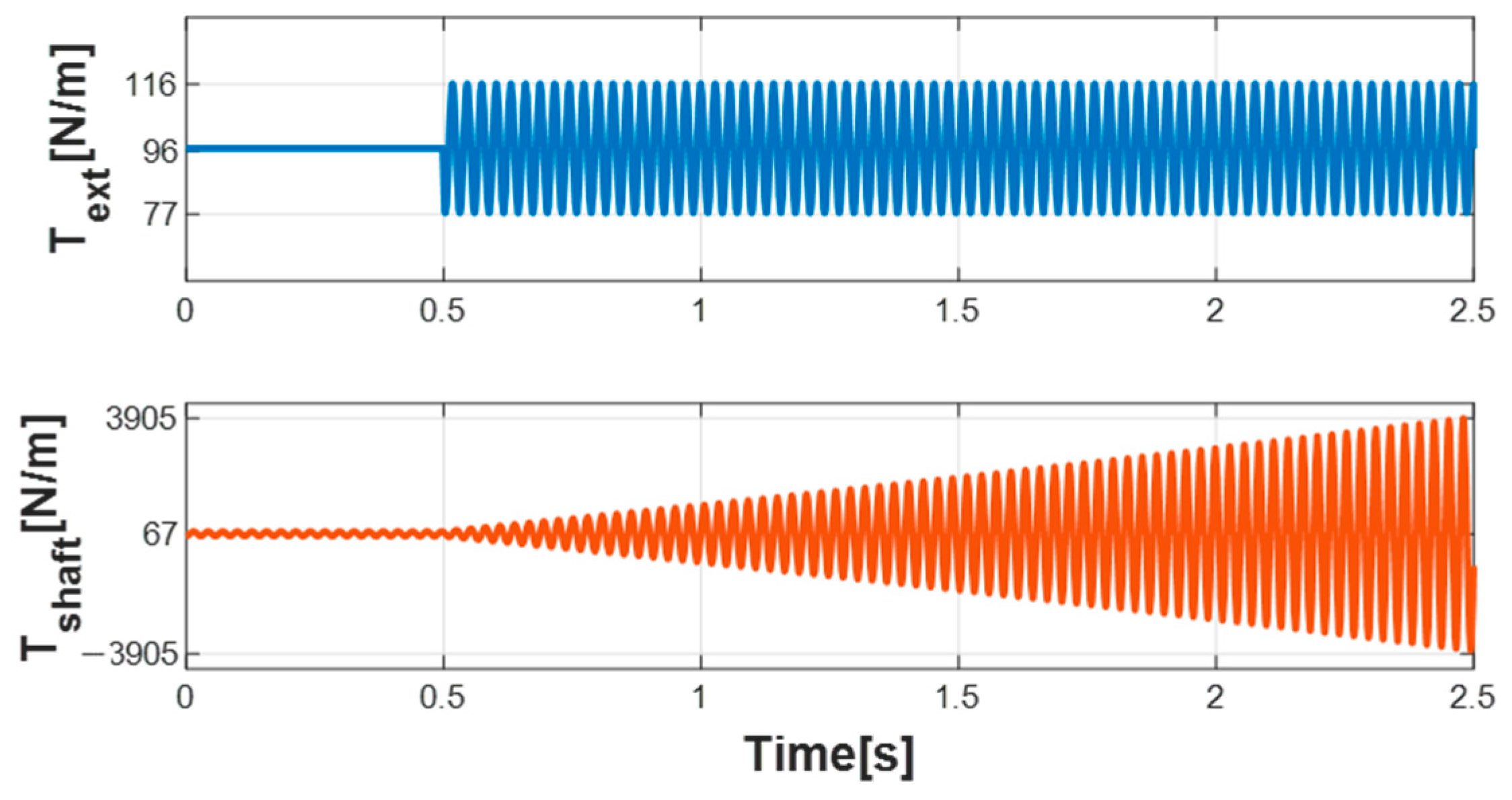
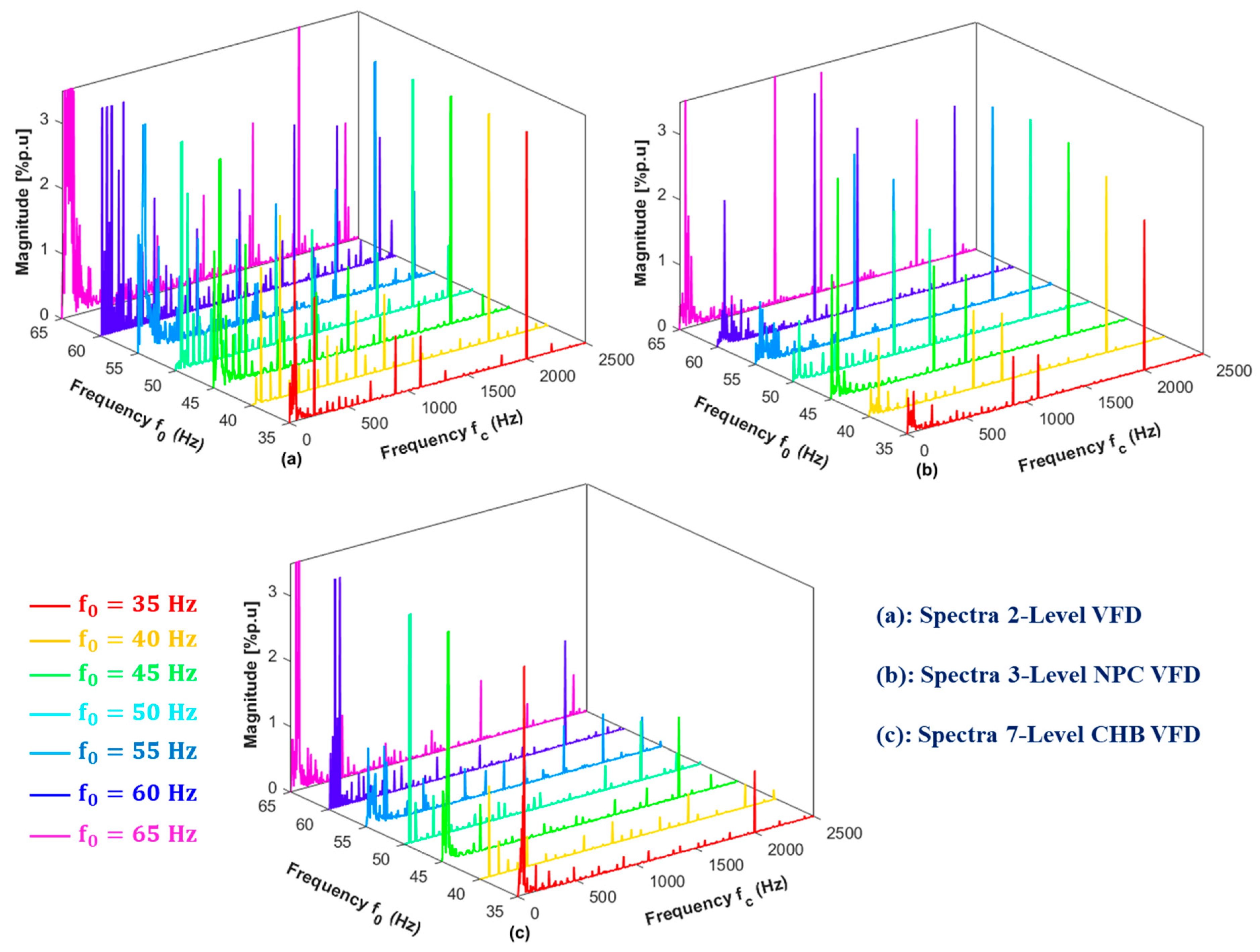
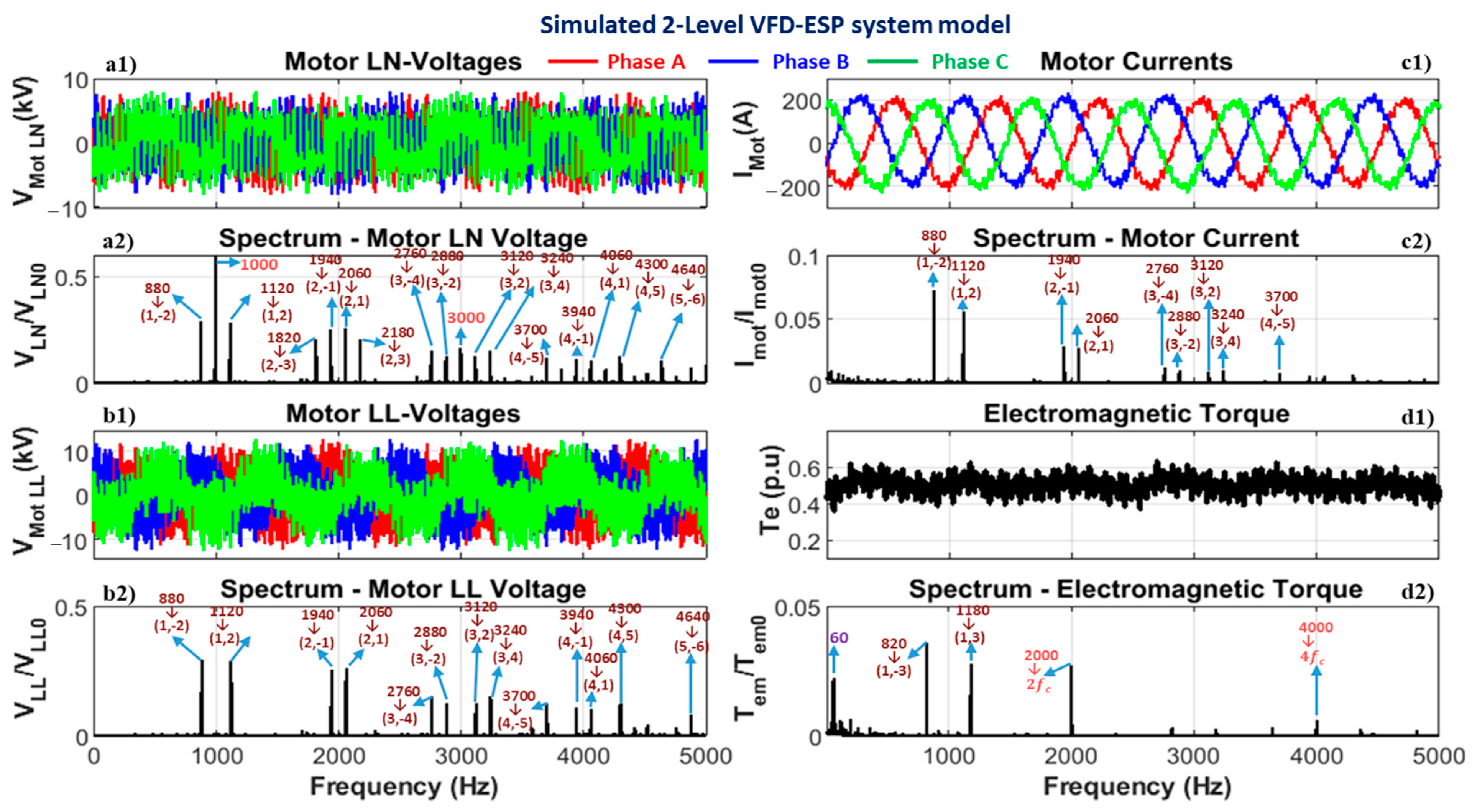
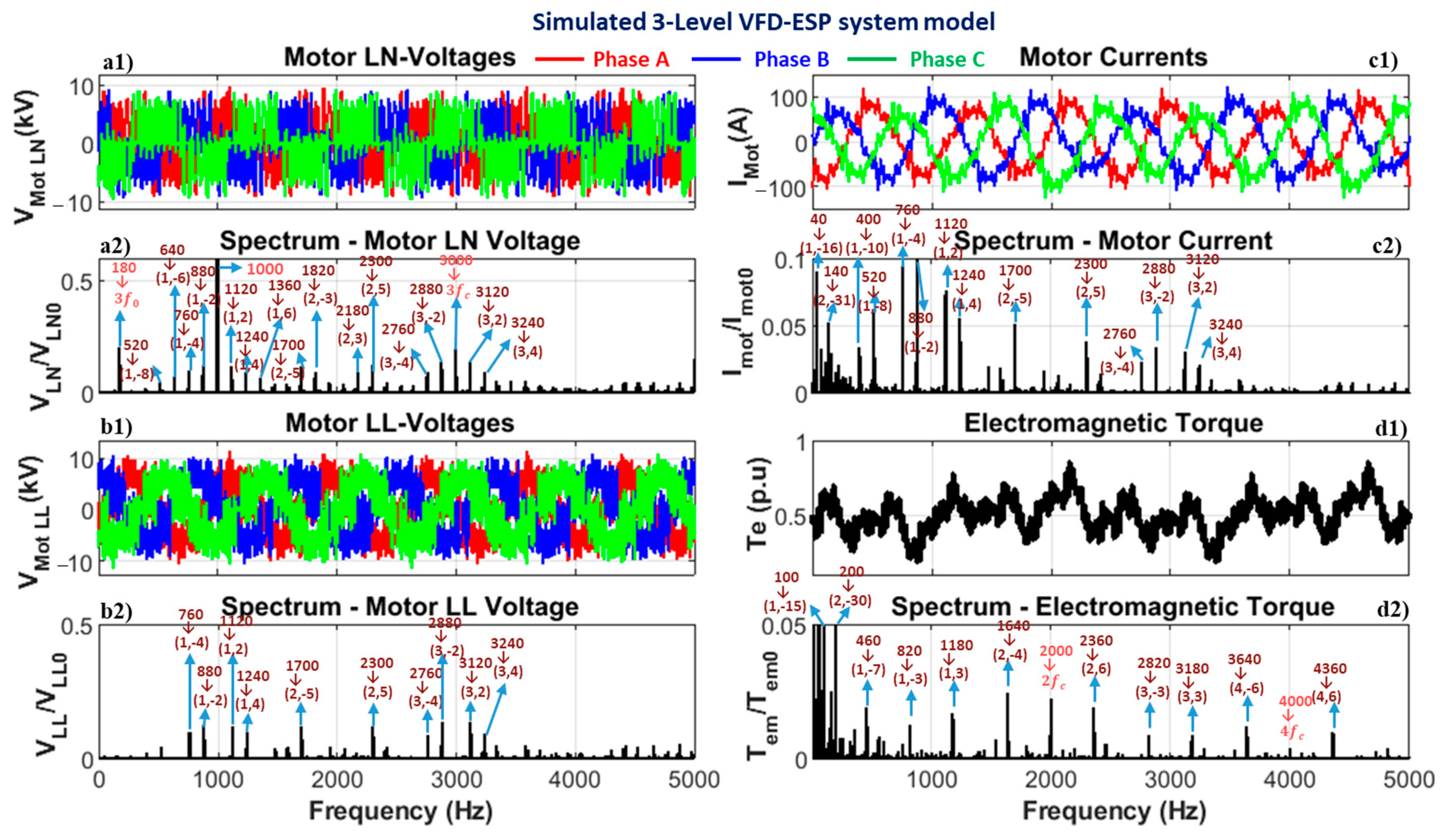
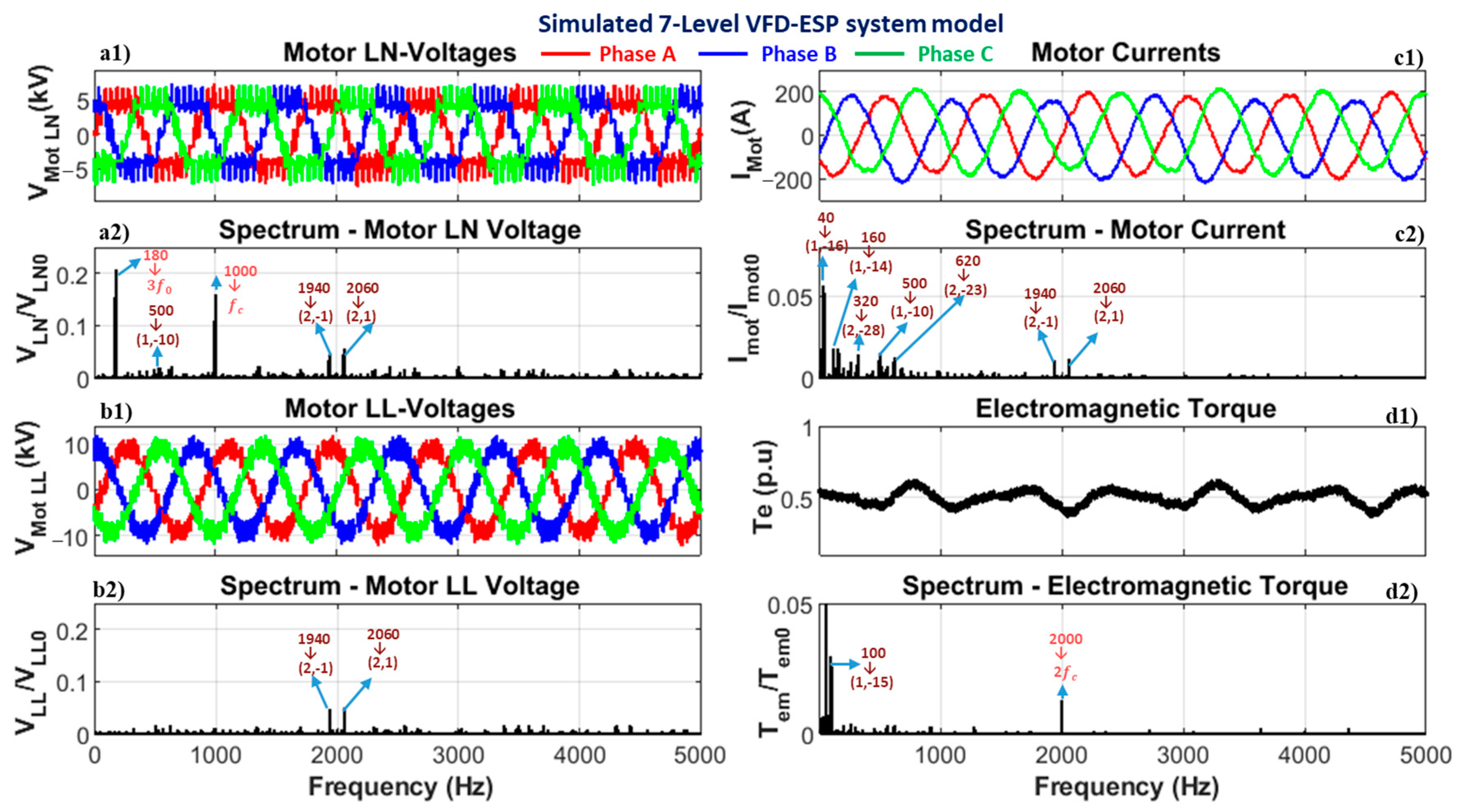
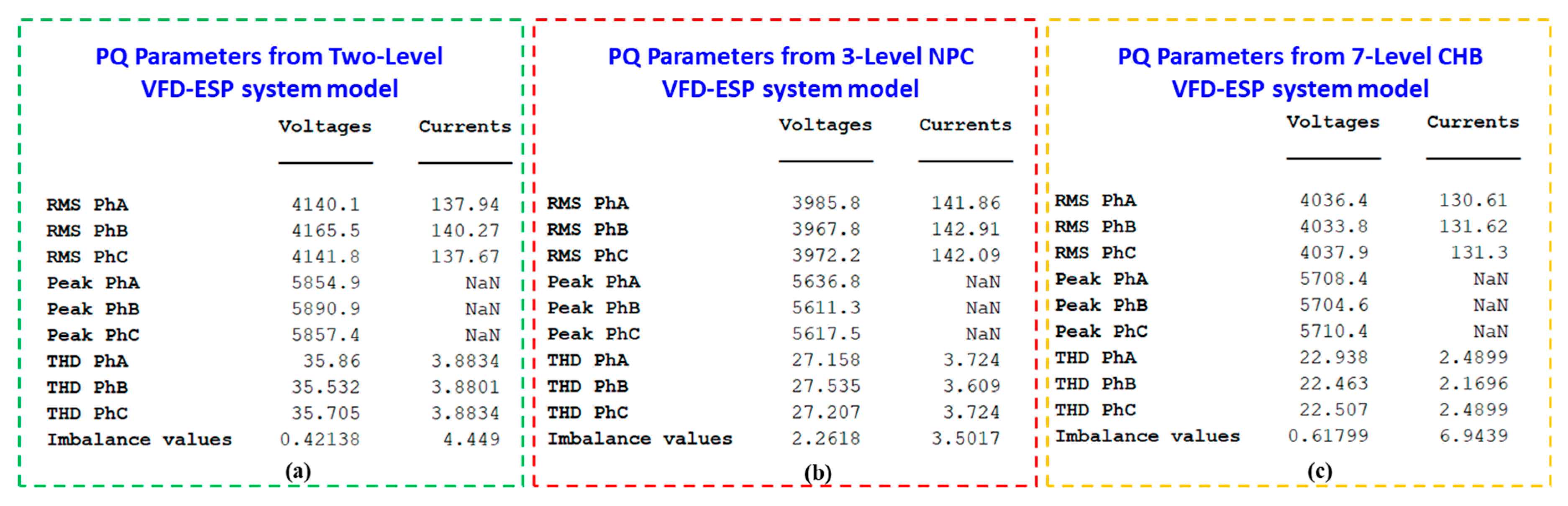
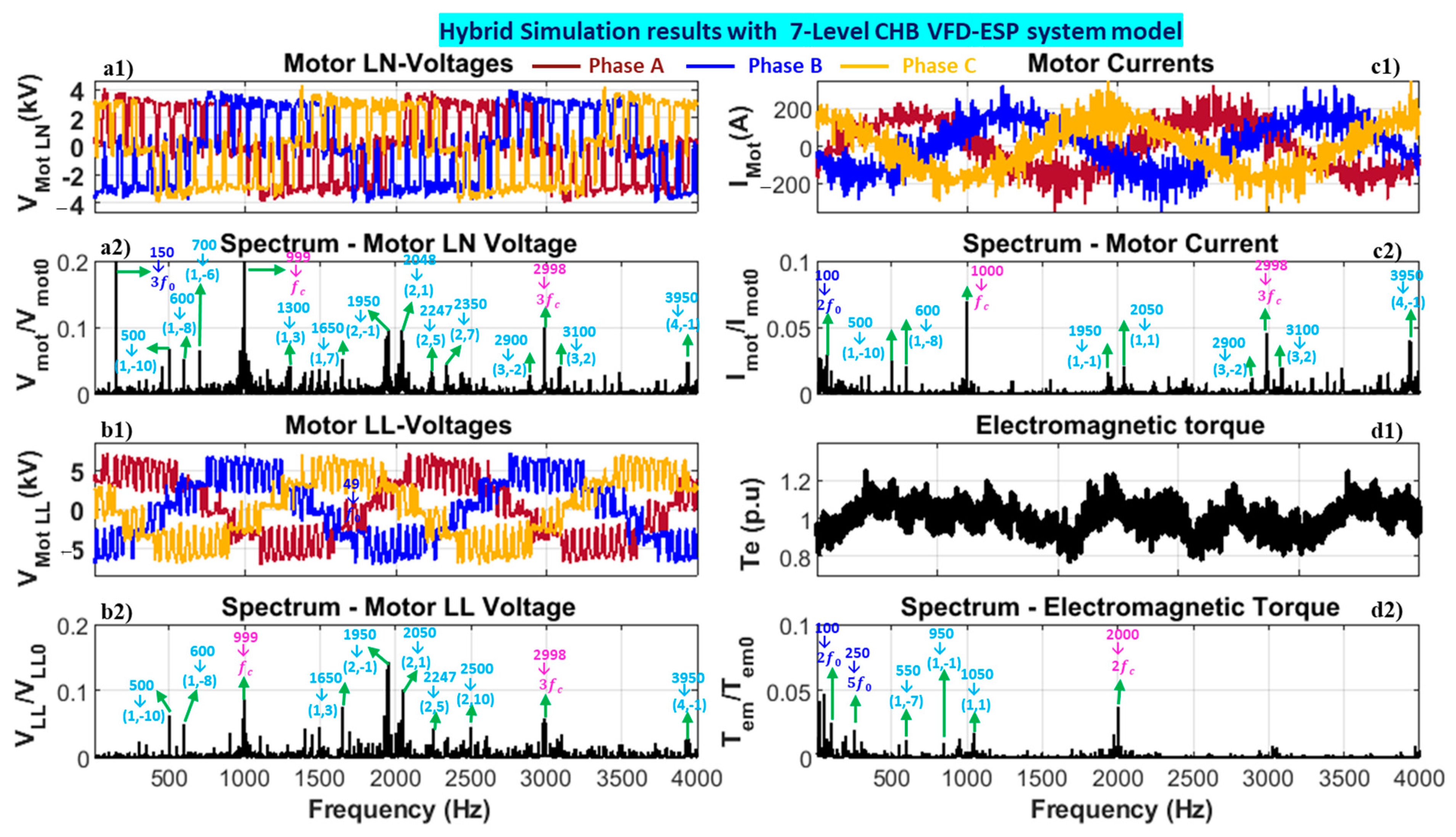
5.3.2. Sample Offline Simulation Results and Discussions

System parameters used for simulated are shown in Appendix A,

Table A1. Simulated parameters.

Cable Electrical Parameters
Length $\left(\mathrm{km}\right)$	1.5
Resistance $\left(\Omega /\mathrm{km}\right)$	0.160
Inductance $\left(\mathrm{mH}/\mathrm{km}\right)$	0.34
Capacitance $\left(\mathsf{\mu }\mathrm{F}/\mathrm{km}\right)$	0.379
PWM VFD parameters
Carrier frequency ($\mathrm{Hz}$)	1000
Fundamental frequency ($\mathrm{Hz}$)	60
ESP motor parameters
Nominal Power $\left(\mathrm{MVA}\right)$	10
Nominal Voltage $\left(\mathrm{V}\right)$	4385
Nominal Current (A)	1860
Nominal Speed $\left(\mathrm{Rpm}\right)$	$1800$
Number of poles	$4$

. More than 1000 operating points have been simulated. The detailed results of specific cases, where $f_c=1 \mathrm{kHz}$ and $f_0=60 \mathrm{kHz}$ are discussed for the three investigated VFD-ESP systems. Sample simulation results for the ESP system with a low-voltage 2-level VFD model are depicted in Figure 27. Similar results for three-level NPC and seven-level CHB ESP systems are shown in Figure 28 and Figure 29, respectively. Each simulated ESP system model shows time and frequency domain results for each state variable. Motor input voltage harmonics are at identical frequencies to VFD-generated harmonics.

As expected, the common-mode voltage (triplen baseband and carrier band) harmonics with a significantly high magnitude in the motor LN-voltages are canceled in the motor LL-voltage. There are no other harmonics in the frequency range of motor LL-voltages. Only the sideband harmonics are present. The impedance of the line cable impacts the sideband harmonics’ amplitudes in the motor current, which are already present in the motor voltage. Families of torque harmonic frequencies match those of the current harmonics that have created them. Sideband current harmonics around an odd multiple of the carrier frequency ${\omega }_c\pm 2{\omega }_0$ produce torque harmonics at ${\omega }_c\pm 3{\omega }_0$. Also, sideband current harmonics around an even multiple of the carrier frequency $2{\omega }_c\pm {\omega }_0$ create torque harmonics at $2{\omega }_c$. A detailed analysis of the motor current and torque harmonic families for a two-level VFD-ESP system (Figure 27(c2,d2)) is provided below for illustrative purposes:

✓

Sideband current harmonics around $1\times$ the PWM frequency $f_c$ are:

   $880=\left|1\times 1000-2\times 60\right|$ Hz, $1120=\left|1\times 1000+2\times 60\right|$ Hz

○

Resulting in sideband torque harmonics around $1\times$ the PWM frequency $f_c$:

$820=\left|1\times 1000-3\times 60\right|$ Hz, $1180=\left|1\ast 1000+3\times 60\right|$ Hz

✓

Sideband current harmonics around $2\times$ the PWM frequency $f_c$ are:

   $1940=\left|2\times 1000-1\times 60\right|$ Hz, $2060=\left|2\times 1000+1\times 60\right|$ Hz

○

Resulting in sideband torque harmonics around $2\times$ the PWM frequency $f_c$ is: $2000=2\times 1000$.

For further power quality study, the key PQ parameters stated in Section 4 were computed from a MATLAB code and then plotted as a table for further PQ analysis at each simulation operating point. The 2-level, 3-level, and 7-level VFD-ESP system models’ measured PQ parameters that were obtained when $f_0=60 \mathrm{Hz}$ are shown in Figure 30a–c, respectively. It can be observed that the measured RMS voltages and currents and Peak voltages in each case are close to their rated values. The 2-level system model, as predicted, presents high THD of voltage and current than the 3-level NPC system model, which exhibits higher THDs than the 7-level CHB system model.

6. Hybrid Real-Time Validations

6.1. Hybrid Real-Time Validation Procedure

The robustness of the proposed model (Figure 26) is evaluated through hybrid real-time simulations. In this validation, the proposed model is divided into (real/analogical) and numerical/digital parts, coupled together and executed in real-time. The idea is to assess the proposed model’s suitability for operational testing using inverter field measurement. The VFD switching function model is replaced in the hybrid real-time simulation with the measured voltage collected from the actual VFD power topology illustrated in Figure 31. The inverter measured voltages were collected from a downscale lab prototype equipped with a 3-level neutral-point-clamped (NPC) VFD inverter based on the Semikron full power module FS3L3R07W2h3f_B11. The prototype also features a set of nine power modules (each H-bridge module is based on a Semikron SK10GD12T4ET package) connected in series to create a 7-level cascaded H-bridge inverter system.

The control hardware is based on Simulink real-time Windows target equipped with a data acquisition board NI-PCI 6229. The measured three-phase inverter output voltages are acquired to the Simulink environment through analog-to-digital (ADC) converter blocks. The following two field scenarios are considered and discussed:

○

NPC VFD power topology operating at the carrier frequency $f_c=1 \mathrm{kHz}$ and fundamental frequency $f_0=50 \mathrm{Hz}$

○

CHB VFD power topology operating at the carrier frequency $f_c=1.5 \mathrm{kHz}$ and fundamental frequency $f_0=50 \mathrm{Hz}$.

At a given operating point, hybrid real-time simulations are run, then the voltages, currents, and airgap electromagnetic torque waveforms are recorded at 50 μs sampling rate for the time and frequency domain analyses. Frequency domain results are obtained by applying a Fast Fourier Transformation (FFT) with a 1 Hz resolution and an even window length to the recorded time-domain results.

6.2. Sample Hybrid Real-Time Simulation Results and Discussions

Figure 32 and Figure 33 show selected hybrid simulation results for the 3-level NPC and 7-level CHB VFD-ESP system models. Each ESP system model is simulated with a short electric cable (20ft) for worst-case harmonic impact at the motor voltage, current and electromagnetic waveforms. The frequencies of each harmonic component in each harmonic family are highlighted, and their magnitudes are magnified to illustrate the precise location of each relevant harmonic component. The impacts of the non-ideal inverter voltage characteristics caused by the ripples in the DC bus voltage are depicted in Figure 32(a1) and Figure 33(a1). Figure 32(b2) and Figure 33(b2) show the impact of the odd/even harmonic in the DC bus voltage on the harmonic distribution of the motor LN-voltages. For instance, by analyzing the results from the 7-level CHB VFD-ESP system model in Figure 33(b1), the odd sideband harmonic components in the first carrier group $\left(1\times f_c\right)$ and the even sideband harmonic components in the second carrier group are given as follows:

✓

Odd sideband voltage harmonics around $1\times$ the PWM frequency $f_c$ (1500 Hz) are: $1448\approx \left|1\times 1500-1\times 50\right|$ Hz, $1548\approx \left|1\times 1500+1\times 50\right|$ Hz.

✓

Even sideband harmonics around $2\times$ the PWM frequency $f_c$ (3000 Hz) are: $2898\approx \left|2\times 1500-2\times 50\right|$ Hz, $3096\approx \left|2\times 1500+2\times 50\right|$ Hz.

Similar harmonics analyses are performed for the results of the hybrid simulation of the 3-level NPC system model in Figure 32(b1). In both cases, the locations of relevant harmonics in motor current are consistent with those in motor voltages. Only their magnitudes are adjusted due to the cable impedance effects. The first and second carrier groups present the even and odd-order sideband current harmonics.

Voltage common-mode components (triplen baseband and carrier band harmonics) are canceled through the differentiation of the line-to-line voltages, but their magnitudes have been significantly reduced. Therefore, the families of electromagnetic torque harmonics produced by each VF-ESP system model are not provided based on the analytical expression of the frequencies derived in Section 3.3.3, where the inverter is assumed to operate with a pure DC component in the DC-bus voltage. In ideal conditions, each electromagnetic harmonic is created by two current harmonic components. However, from Figure 32(d2) and Figure 33(d2), new harmonic components are present in the electromagnetic torque spectrum due to the interaction between the DC bus voltage harmonics and the inverter PWM voltage harmonics. Overall, hybrid simulation results are also crucial to carefully evaluate how harmonics from inverter field voltage measurements propagate through the transmission cable so that their effects on the quality of the power being supplied to the ESP motor can be assessed prior to installation of the entire system.

7. Conclusions

This paper proposes a unified approach to understanding how variable frequency drives (VFDs) impact the power quality of an Electric Submersible Pump (ESP) supplied through a transmission cable. It also explains how VFDs might excite mechanical-shaft torsional modes in such applications. The paper outlines easy-to-follow procedures for system integration analyses of such configurations, including torsion vibration analysis. Time-domain and frequency-domain switching function models of two-level, three-level neutral-point-clamped, and cascaded H-bridge multilevel VFD inverter topologies are proposed for this purpose. Simulating VFD-ESP systems is time-consuming and requires complex skill sets to design, model, and implement in simulation software. Therefore, a simplified time-domain model is proposed to reproduce the steady-state behavior of low- and medium-voltage ESP systems supplied by PWM-VFD topologies at various operating points in normal and failure modes. The investigated failure mode in this research is when an ESP system is powered by a CHB-VFD topology operating with one or more damaged and bypassed power modules. Under failure mode, the neutral-shift PWM technique is applied by modifying the PWM reference voltage angles. The neutral-shift strategy produces balanced inverter output line voltages and currents even if its phase voltages are unbalanced due to the failed cells.

Offline and hybrid real-time simulation results at different operating points support the accuracy of the proposed simplified VFD-ESP system model. Results are generated in time and frequency domains, as well as main power quality parameters, such as RMS and Peak voltages, voltage and current THDs, maximum dv/dt, voltage, and current imbalances. In all simulated cases studied, voltage, current, and motor airgap torque harmonic components induced by the three investigated VFD topologies are derived and correlated to the theoretical predictions. In addition, the effects of the electrical and mechanical spectrum modification using a neutral-shift control strategy under failed cells are highlighted and discussed. Overall, simulation results match the theoretical calculation with acceptable accuracy, regardless of the selected operating points or carrier frequencies.

References

1. Ding, L.; Li, W.Y.; Zargari, N.R.; Paes, R. Sensorless Control of CSC-Fed PMSM Drives with Low Switching Frequency for Electrical Submersible Pump Application. IEEE Trans. Ind. Appl. 2020, 56, 3799–3808. [Google Scholar] [CrossRef]
2. Fonsêca, D.A.; Salazar, A.O.; Villarreal, E.R.; Espinoza, G.A. Downhole Telemetry Systems to Monitor Electric Submersible Pumps Parameters in Oil Well. IEEE Access 2021, 9, 12824–12839. [Google Scholar] [CrossRef]
3. Romero, O.J.; Hupp, A. Subsea Electrical Submersible 1 Pump Significance in Petroleum 2 3 Offshore Production. J. Energy Resour. Technol. 2013, 136, 012902. [Google Scholar] [CrossRef]
4. Cortes, B.; Araujo, L.R.; Penido, D.R. Electrical submersible pump system model to assist oil lifting studies. J. Petrol. Sci. Eng. 2019, 174, 1279–1289. [Google Scholar] [CrossRef]
5. Smith, J.R.; Grant, D.M.; Al-Mashgari, A.; Slater, R.D. Operation of subsea electrical submersible pumps supplied over extended length cable systems. IEE Proc. Electr. Power Appl. 2000, 147, 544–552. [Google Scholar] [CrossRef]
6. Allen-Bradley. PowerFlex Medium Voltage AC Drives Bulletin Numbers 6000G, 6000T, 7000A, 7000, and 7000L; Rockwell Automation: Laval, QC, Canada, 2022. [Google Scholar]
7. Liang, X.; Kar, N.C.; Liu, J. Load Filter Design Method for Medium-Voltage Drive Applications in Electrical Submersible Pump Systems. IEEE Trans. Ind. Appl. 2015, 51, 2017–2029. [Google Scholar] [CrossRef]
8. Liang, X.; El-Kadri, A. Operational Parameters Affecting Harmonic Resonance in Electrical Submersible Pump Systems. IEEECan. J. Electr. Comput. Eng. 2019, 42, 183–197. [Google Scholar] [CrossRef]
9. Gabor, T. Electrical Submersible Pump Components and Their Operational Features. In Electrical Submersible Pumps Manual, 2nd ed.; Gabor, T., Ed.; Elsevier: Amsterdam, The Netherlands, 2018; pp. 55–152. [Google Scholar]
10. Pragale, R.; Shipp, D.D. Investigation of premature ESP failures and oil field harmonic analysis. IEEE Trans. Ind. Appl. 2018, 53, 3175–3181. [Google Scholar] [CrossRef]
11. Tamer, A.; Shipp, D.; Dionise, T. Reducing electrical submersible pump downtime by mitigation of VSD output power quality problems. In Proceedings of the IEEE Petroleum and Chemical Industry Committee Conference (PCIC), Vancouver, BC, Canada, 9–12 September 2019. [Google Scholar]
12. Weixiong, J.; Honghui, W.; Guijie, L.; Yonghong, L.; Baoping, C.; Zhixiong, L. A Novel Method for Mechanical Fault Diagnosis of Underwater Pump Motors Based on Power Flow Theory. IEEE Trans. Instrum. Meas. 2021, 70, 1–17. [Google Scholar]
13. Rabbi, S.F.; Kahnamouei, J.T.; Liang, X.; Yang, J. Shaft Failure Analysis in Soft-Starter Fed Electrical Submersible Pump Systems. IEEE Open J. Ind. Appl. 2019, 1, 1–10. [Google Scholar] [CrossRef]
14. Neumann, K.C.; La, D.; Yoo, H.; Burkepile, E. Programmable Autonomous Water Samplers (PAWS): An inexpensive, adaptable, and robust submersible system for time-integrated water sampling in freshwater and marine ecosystems. HardwareX 2023, 13, e00392. [Google Scholar] [CrossRef] [PubMed]
15. Shipp, D.D.; Voytechek, M.; Morganson, S. Power Quality Survey for Shell Canada’s Virginia Hills Oil Field. In Electrical Submersible Pump Workshop Record: Society of Petroleum Engineers; SPE Mid-Continent Operations Symposium: Oklahoma, OK, USA, 1996. [Google Scholar]
16. Farbis, M.; Hoevenaars, A.H.; Greenwald, J.L. Oil field retrofit of ESPs to Meet Harmonic Compliance. In Proceedings of the IEEE Petroleum and Chemical Industry Technical Conference (PCIC), San Francisco, CA, USA, 8–10 September 2014. [Google Scholar]
17. Hoevenaars, A.H.; McGraw, M.; Alexander, J. Rightsizing Generators Through Harmonic Mitigation Realizes Energy, Emissions, and Infrastructure Reductions. IEEE Trans. Ind. Appl. 2017, 53, 675–683. [Google Scholar] [CrossRef]
18. Song-Manguelle, J.; Ekemb, G.; Mon-Nzongo, D.; Tao, J.; Doumbia, M.L. A Theoretical Analysis of Pulsating Torque Components in AC Machines with Variable Frequency Drives and Dynamic Mechanical Loads. IEEE Trans. Ind. Electron. 2018, 65, 9311–9324. [Google Scholar] [CrossRef]
19. Mon-Nzongo, D.; Ekemb, G.; Song-Manguelle, J. LCIs and PWM-VSIs for the Petroleum Industry: A Torque Oriented Evaluation for Torsional Analysis Purposes. IEEE Trans. Power Electron. 2019, 34, 8956–8970. [Google Scholar] [CrossRef]
20. Ekemb, G.; Slaoui-Hasnaoui, F.; Song-Manguelle, J.; Lingom, M.P.; Fofana, I. Instantaneous electromagnetic torque components in synchronous motor fed by load-commutated inverters. Energies 2021, 14, 3223. [Google Scholar] [CrossRef]
21. Pindoriya, R.M.; Thakur, R.K.; Rajpurohit, B.S.; Kumar, R. Numerical and Experimental Analysis of Torsional Vibration and Acoustic Noise of PMSM Coupled with DC Generator. IEEE Trans. Ind. Electron. 2022, 69, 3345–3356. [Google Scholar] [CrossRef]
22. Nassif, A.B. Assessing the Impact of Harmonics and Interharmonics of Top and Mudpump Variable Frequency Drives in Drilling Rigs. IEEE Trans. Ind. Appl. 2019, 55, 5574–5583. [Google Scholar] [CrossRef]
23. API. API Standard 617, Axial and Centrifugal Compressors and Expander-Compressors, 8th ed.; API: Englewood, CO, USA, 2016. [Google Scholar]
24. API. API Standard 672, Packaged, Integrally Geared Centrifugal Air Compressors for Petroleum, Chemical, and Gas Industry Services, 5th ed.; API: Englewood, CO, USA, August 2019. [Google Scholar]
25. Submersible Pump Engineering. Unbalanced currents and submersible motors. SMENG 2002, 1–2. [Google Scholar]
26. Reed, J.A. Investigation and Modeling of Voltage and Current Unbalance on a Three-Phase Submersible Pump. Master’s Thesis, The University of Texas at Arlington, Arlington, TX, USA, 2013; pp. 1–167. [Google Scholar]
27. Lingom, P.M.; Song-Manguelle, J.; Mon-Nzongo, D.L.; Flesch, R.C.; Tao, J. Analysis, and control of PV cascaded h-bridge multilevel inverter with failed cells and changing meteorological conditions. IEEE Trans. Power. Electron. 2020, 36, 1777–1789. [Google Scholar] [CrossRef]
28. Carnielutti, F.; Pinheiro, H.; Rech, C. Generalized carrier-based modulation strategy for cascaded multilevel converters operating under fault conditions. IEEE Trans. Ind. Electron. 2012, 59, 679–689. [Google Scholar] [CrossRef]
29. API. API Standard 673, Centrifugal Fans for Petroleum, Chemical and Gas Industry Services, 3rd ed.; API: Englewood, CO, USA, December 2014. [Google Scholar]
30. API. API Standard 684, Paragraphs Rotodynamic Tutorial: Lateral Critical Speeds, Unbalance Response, Stability, Train Torsional, and Rotor Balancing, 2nd ed.; API Recommended Practice 684; API: Englewood, CO, USA, August 2005. [Google Scholar]
31. Ong, C.M. Dynamic Simulation of Electric Machinery Using Matlab/Simulink. Can. J. Electr. Comput. Eng. 2019, 42, 183–197. [Google Scholar]
32. Song-Manguelle, J.; Sihler, C.; Nyobe-Yome, J.M. Modeling of Torsional Resonances for Multi-Megawatt Drives Design. IEEE Trans. Ind. Electron. 2018, 65, 9311–9324. [Google Scholar] [CrossRef]
33. Lingom, P.M.; Song-Manguelle, J.; Doumbia, M.L.; Flesch, R.C.; Tao, J. Electrical Submersible Pumps: A System Modeling Approach for Power Quality Analysis with Variable Frequency Drives. IEEE Trans. Power. Electron. 2022, 37, 7039–7054. [Google Scholar] [CrossRef]
34. Liang, X. Linearization approach for modeling power electronics devices in power systems. IEEE J. Emerg. Sel. Top. Power Electron. 2014, 2, 1003–1012. [Google Scholar] [CrossRef]
35. Han, X.; Palazzolo, A.B. VFD machinery vibration fatigue life and multi-level inverter effect. IEEE Trans. Ind. Appl. 2013, 49, 2562–2575. [Google Scholar] [CrossRef]
36. Feletto, F.; Durham, R.A.; da Costa Bortoni, E.; de Carvalho Costa, J.G. Improvement of MV Cascaded H-Bridge Inverter (CHBI) VFD Availability for High-Power ESP Oil Wells. IEEE Trans. Ind. Appl. 2018, 55, 1006–1011. [Google Scholar] [CrossRef]
37. Busacca, A.; Di Tommaso, A.O.; Miceli, R.; Nevoloso, C.; Schettino, G.; Scaglione, G.; Viola, F.; Colak, I. Switching Frequency Effects on the Efficiency and Harmonic Distortion in a Three-Phase Five-Level CHBMI Prototype with Multicarrier PWM Schemes: Experimental Analysis. Energies 2022, 15, 586. [Google Scholar] [CrossRef]
38. Qin, F.; Gao, F.; Tang, Y.; Wang, J.; Xu, T. Comprehensive comparisons between six-arm and nine-arm modular multilevel converter. CPSS Trans. Power Electron. Appl. 2020, 5, 135–146. [Google Scholar] [CrossRef]
39. Anderson, J.A.; Zulauf, G.; Kolar, J.W.; Deboy, G. New Figure-of-Merit Combining Semiconductor and Multi-Level Converter Properties. IEEE Open J. Power Electron. 2020, 1, 322–338. [Google Scholar] [CrossRef]
40. Yifei, L.; Fei, X.; Wang, B.; Binli, L. Failure Analysis of Power Electronic Devices and Their Applications under Extreme Conditions. Chin. J. Electr. Eng. 2016, 2, 91–100. [Google Scholar]
41. Holmes, D.G.; Lipo, T.A. PulseWidth Modulation for Power Converters, Principles and Practice; IEEE Press: Piscataway, NJ, USA, 2003. [Google Scholar]
42. Gary, W.C.; Shin-Kuan, C. An Analytical Approach for Characterizing Harmonic and Interharmonic Currents Generated by VSI-Fed Adjustable Speed Drives. IEEE Trans. Power Deliv. 2005, 20, 2585–2593. [Google Scholar]
43. Soltani, H.; Davari, P.; Zare, F.; Blaabjerg, F. Effects of Modulation Techniques on the Input Current Interharmonics of Adjustable Speed Drives. IEEE Trans. Ind. Electron. 2018, 65, 165–178. [Google Scholar] [CrossRef] [Green Version]
44. Hota, A.; Agarwal, V. Novel Three-Phase H10 Inverter Topology with Zero or Constant Common-Mode Voltage for Three-Phase Induction Motor Drive Applications. IEEE Trans. Ind. Electron. 2022, 69, 7522–7525. [Google Scholar] [CrossRef]
45. Xiaoling, X.; Xiongfei, W.; Dong, L.; Blaabjerg, F.; Chengyong, Z. Common-Mode Insertion Indices Compensation with Capacitor Voltages Feedforward to Suppress Circulating Current of MMCs. CPSS Trans. Power. Electron. Appl. 2020, 5, 103–113. [Google Scholar]
46. Song-Manguelle, J.; Ekemb, G.; Schroder, S.; Geyer, T.; Nyobe-Yome, J.M.; Wamkeue, R. Analytical expression of pulsating torque harmonics due to PWM drives. In Proceedings of the IEEE Energy Conversion Congress and Exposition, Denver, CO, USA, 15–19 September 2013. [Google Scholar]
47. Std 1159-2019; IEEE Recommended Practice for Monitoring Electric Power Quality. IEEE: Piscataway, NJ, USA, 2019.
48. NEMA Std and Publication MG-1-2009 Motor and Generators; National Electrical Manufacturers Association: Rosslyn, UK, 2019.
49. Masoum, M.A.; Fuchs, E.F. Power Quality in Power Systems and Electrical Machines, 2nd ed.; Academic Press, Elsevier: London, UK, 2008. [Google Scholar]
Figure 1. A generic system configuration of an Electric Submersible Pump.
Energies 16 05121 g001
Figure 2. Investigated VFD topologies: (a) Low-Voltage 2-Level VFD Inverter; (b) Medium-Voltage 3-Level NPC VFD Inverter; (c) Medium-Voltage Multilevel CHB VFD Inverter.
Energies 16 05121 g002
Figure 3. Some possible VFD output power quality issues.
Energies 16 05121 g003
Figure 4. Typical electric power configuration of an ESP system.
Energies 16 05121 g004
Figure 5. Single-line diagram of electrical ESP system model.
Energies 16 05121 g005
Figure 6. Resonance phenomenon in single series RLC circuit: (a) Schematic diagram; (b): Resonance curves.
Energies 16 05121 g006
Figure 7. A one-inertia system.
Energies 16 05121 g007
Figure 8. Shaft’s torque behavior (top) Externally applied torque pulsating at a shaft’s eigenfrequency; (bottom) Shaft excited response.
Energies 16 05121 g008
Figure 9. A generic arrangement of a shaft system with multi-mass.
Energies 16 05121 g009
Figure 10. Phenomenological electric analogy of the shaft system.
Energies 16 05121 g010
Figure 11. Investigated VFD topologies for ESP and their PWM strategies and corresponding switching waveforms: (a1–a5) For the two-level VFD; (b1–b5) For the three-level NPC VFD; (c1–c5) For the multilevel CHB VFD.
Energies 16 05121 g011
Figure 12. VFD switching models: (a) Two-level VFD switching model; (b); Three-level NPC VFD switching model; (c) Multilevel CHB VFD switching model.
Energies 16 05121 g012
Figure 13. Neutral-shift strategy for a CHB inverter system with faulted cells.
Energies 16 05121 g013
Figure 14. Voltage phasor diagram for different operation modes: (a) Normal model; (b) Corrected mode.
Energies 16 05121 g014
Figure 15. General VFD output voltage harmonic families: (a) Line-to-Neutral voltage harmonics families; (b) Line-to-Line voltage harmonics.
Energies 16 05121 g015
Figure 16. Electromagnetic torque model of a motor [33].
Energies 16 05121 g016
Figure 17. A generic Campbell diagram for a motor supplied by a PWM-VSI.
Energies 16 05121 g017
Figure 18. Definition of dv/dt.
Energies 16 05121 g018
Figure 19. Sample comparison simulation results between the two-level VFD and its simplified model both in time and frequency domains at fc = 1 kHz and f0 = 60 Hz. (a) Time domain; (b) Frequency domain.
Energies 16 05121 g019
Figure 20. Sample comparison simulation results between the three-level NPC VFD and its simplified model both in time and frequency domains at fc = 1 kHz and f0 = 60 Hz. (a) Time domain; (b) Frequency domain.
Energies 16 05121 g020
Figure 21. Sample comparison simulation results between the seven-level CHB VFD and its simplified model both in time and frequency domains at fc = 1 kHz and f0 = 60 Hz. (a) Time domain; (b) Frequency domain.
Energies 16 05121 g021
Figure 22. Operational range spectra of the line-to-neutral voltage generated by (a) Two-level VFD; (b) Three-level NPC VFD, and (c) seven-level CHB VFD, with f c = 1   kHz for all cases.
Energies 16 05121 g022
Figure 23. Time-domain voltage waveforms of a CHB-VFD under normal and corrected modes. (a1–a3) Normal mode; (b1–b3) Corrected mode.
Energies 16 05121 g023
Figure 24. Spectra of the phase output voltages of a CHB-VFD under normal and corrected modes. (a1a3) Normal mode; (b1b3) Corrected mode.
Energies 16 05121 g024
Figure 25. Spectra of the line output voltages of a CHB-VFD under normal and corrected modes. (a1a3) Normal mode; (b1b3) Corrected mode.
Energies 16 05121 g025
Figure 26. Integration of subsystem models for numerical validation purposes.
Energies 16 05121 g026
Figure 27. Simulation results of two-level VFD ESP system model with f c = 1   kHz ; f 0 = 50   Hz : (a1) motor LN-voltages; (a2) Spectrum of motor LN-voltage; (b1) Motor LL-voltages; (b2) Spectrum of motor LN-voltage; (c1) Motor currents; (c2) Spectrum of motor current; (d1) Motor electromagnetic torque; (d2) Spectrum of motor electromagnetic.
Energies 16 05121 g027
Figure 28. Simulation results of three-level NPC VFD ESP system model with f c = 1   kHz ; f 0 = 60   Hz : (a1) Motor LN-voltages; (a2) Spectrum of motor LN-voltage; (b1) Motor LL-voltages; (b2) Spectrum of motor LN-voltage; (c1) Motor currents; (c2) Spectrum of motor current; (d1) Motor electromagnetic torque; (d2) Spectrum of motor electromagnetic.
Energies 16 05121 g028
Figure 29. Simulation results of seven-level CHB VFD ESP system model with f c = 1   kHz ; f 0 = 60   Hz : (a1) Motor LN-voltages; (a2) Spectrum of motor LN-voltage; (b1) Motor LL-voltages; (b2) Spectrum of motor LN-voltage; (c1) Motor currents; (c2) Spectrum of motor current; (d1) Motor electromagnetic torque; (d2) Spectrum of motor electromagnetic.
Energies 16 05121 g029
Figure 30. Measured PQ parameters obtained from each simulated ESP system model at f c = 1   kHz   and f 0 = 60   Hz : (a) Two-level VFD-ESP model; (b) Three-level NPC VFD-ESP model; (c) Seven-level CHB VFD-ESP model.
Energies 16 05121 g030
Figure 31. Validation principle of Hybrid real-time simulation results.
Energies 16 05121 g031
Figure 32. Hybrid simulation results of three-level NPC VFD ESP system model with f c = 1   kHz ; f 0 = 50   Hz : (a1) Motor LN-voltages; (a2) Spectrum of motor LN-voltage; (b1) Motor LL-voltages; (b2) Spectrum of motor LN-voltage; (c1) Motor currents; (c2) Spectrum of motor current; (d1) Motor electromagnetic torque; (d2) Spectrum of motor electromagnetic.
Energies 16 05121 g032
Figure 33. Hybrid simulation results of seven-level CHB VFD ESP system model with f c = 1.5   kHz ; f 0 = 50   Hz : (a1) Motor LN-voltages; (a2) Spectrum of motor LN-voltage; (b1) Motor LL-voltages, (b2) Spectrum of motor LN-voltage; (c1) Motor currents; (c2) spectrum of motor current; (d1) Motor electromagnetic torque; (d2) Spectrum of motor electromagnetic.
Energies 16 05121 g033